Satellite Hyperspectral Mapping of Farmland Soil Organic Carbon in Yuncheng Basin Along the Yellow River, China

Abstract

This study combined field survey data with Gaofen 5 (GF-5) satellite hyperspectral images of the Yuncheng Basin (China), considering 15 environmental variables. Random forest (RF) was used to select the optimal satellite hyperspectral model, sequentially introducing natural and farmland management factors into the model to analyze the spatial distribution of farmland soil organic carbon (SOC). Furthermore, RF factorial experiments determined the contributions of farmland management, climate, vegetation, soil, and topography to the SOC. Structural equation modeling (SEM) elucidated the driving mechanisms of SOC variations. Integrating satellite hyperspectral data and environmental variables improved the prediction accuracy and SOC-mapping precision of the model. The integration of natural variables significantly improved the RF model performance (R² = 0.78). The prediction accuracy enhanced with the introduction of crop phenology (R² = 0.81) and farmland management factors (R² = 0.87). The model that incorporated all 15 variables demonstrated the highest prediction accuracy (R² = 0.89) and greatest spatial SOC variability, with minimal uncertainty. Farmland management activities exerted the strongest influence on SOC (0.38). The proposed method can support future investigations on soil carbon sequestration processes in river basins worldwide.

1. Introduction

Soil acts as both a global carbon source and a sink. Farmland soil, influenced by natural conditions and agricultural management practices, is a key topic in global carbon cycle research [1]. High-precision mapping of farmland soil organic carbon (SOC) enables the precise localization of soil carbon distribution, thereby facilitating optimized agricultural planning. Notably, high-precision mapping can support the development of targeted strategies for regional ecosystem stability, increased crop yield, and sustainable agricultural development.

According to the soil-forming factors theory [2], soil is a product of the combined effects of parent material, climate, organisms, topography, and time. In 2003, McBratney [3] synthesized previous research to propose the Scorpan model, which conceptualizes target soil types and properties as a functional relationship of multiple environmental variables (including climate, human activities, parent material, topography, soil properties, and spatial position). Digital soil mapping (DSM) leverages these environmental covariates to effectively predict and spatially map soil types and properties at regional, national, and global scales [4]. Currently, DSM based on soil-landscape models is used globally for mapping large-scale soil properties, such as soil organic matter (SOM) [5], SOC [6,7], pH [8], and bulk density [9]. However, at smaller scales (e.g., field plots), variations in factors (such as topography and climate) may be small, necessitating the identification of more sensitive variables related to human activities, such as farmland management practices [10]. These practices directly influence the input, output, and transformation rates of carbon in farmland soils, affecting the SOC content and spatial distribution [11]. Previous studies on phenological parameters [12] and cropping system patterns [13] have demonstrated the effectiveness of incorporating farmland management activities in SOC mapping. Therefore, integrating agricultural management information has the potential to reveal dynamic changes in farmland SOC and improve the prediction accuracy of DSM. Traditional methods for collecting farmland planting and management information are time-consuming and labor-intensive and often lack spatial detail. In contrast, remote sensing (RS) technology offers rapid, accurate, and spatially extensive data acquisition. Therefore, this technology offers an effective means for obtaining large-scale farmland planting and management information [14]. Wu [15] identified farmland planting and management factors (e.g., crop type, cropping index, and straw incorporation) as effective environmental variables for predicting SOC in the Jianghan Plain in China, revealing significant differences in dominant controlling factors across various scales. Wang et al. [16] analyzed farmland soil samples from northern China, considering five categories of environmental covariates (climate, vegetation, topography, soil properties, and agricultural management), to map farmland SOC distribution across the region.

Notably, a limitation of environmental variables used for predicting the spatial variability of SOC is their high spatial similarity across diverse geographical environments, particularly at the regional scale, where these variables often poorly respond to subtle SOC changes. Laboratory, airborne, and satellite hyperspectral data have gradually become important data sources for DSM [17,18]. Numerous previous studies have demonstrated the feasibility of using visible-near infrared (Vis-NIR) spectroscopy for estimating soil properties at the regional scale [19]. Although laboratory hyperspectral data generally offer higher estimation accuracy, they cannot provide continuous spatial information for predicting and mapping soil properties across entire regions [20]. Furthermore, airborne hyperspectral data are constrained by expensive instrumentation and limitations in flight coverage and timing, restricting related studies to relatively small areas [21]. High spectral and spatial resolution data are essential for conducting fine-scale quantitative assessments of SOC [22]. Currently, GF-5 and CHRIS are the most commonly used satellite hyperspectral data for SOC/SOM inversion [23]. Thus, while environmental variables can explain the driving mechanisms and spatial patterns of SOC variation, hyperspectral data overcomes the limitation of ‘indirect correlation’ inherent in environmental variables through direct detection of SOC’s chemical spectral characteristics. The integration of both approaches achieves a systematic framework for SOC micro-variation analysis, enabling ‘precise identification—mechanistic interpretation—spatial mapping’.

The soils in the Yellow River Basin in China are typically coarse-textured and loose and exhibit poor vertical structures exacerbated by soil erosion. The presence of substantially sloping farmlands further limits high-quality agricultural development in the region. Therefore, high-precision prediction and spatial distribution mapping of farmland soil organic carbon (SOC) are of great significance for precision soil management and agricultural production, yet relevant information remains scarce. The aims of this study were to do the following:

(1)

Integrate input predictors (satellite hyperspectral data, classical factors, and farmland management factors) into a random forest (RF) model to generate fine-resolution spatial maps of farmland SOC across the study region. Explore the impact of different combinations of soil satellite hyperspectral data and environmental variables on the SOC-prediction accuracy of the model.

(2)

Evaluate the prediction accuracy of and uncertainties in the farmland SOC spatial distribution map and investigate the effectiveness of different environmental variables, particularly farmland management, in predicting the farmland SOC across the region.

(3)

Conduct RF factorial experiments to determine the associations and relative contributions of five environmental factor categories (farmland management activities, topography, vegetation, climate, and soil) to farmland SOC across the study region. Employ structural equation modeling (SEM) to analyze the direct and indirect influences among these five categories and their constituent factors.

2. Materials and Methods

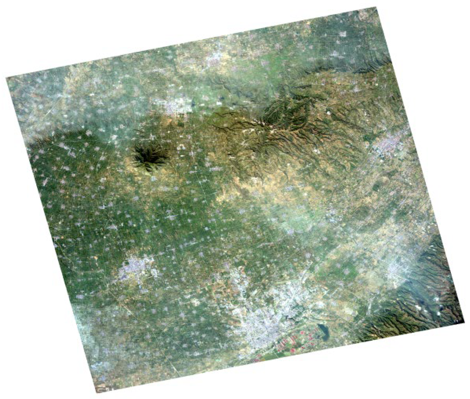
2.1. Study Area

The study area is located in the northern part of the Yuncheng Basin along the middle reaches of the Yellow River, in Yuncheng City, Shanxi Province, China (Figure 1). Administratively, it primarily includes parts of the Jishan, Xinjiang, Wanrong, Wenxi, Xia, and Linyi counties and the Yanhu district. The terrain features minor mountainous and hilly areas. The total study area covers approximately 5304.74 km², corresponding to the footprint of one Geofen 5 (GF-5) image (Figure 2). The farmland types in this region include dryland, irrigated land, and sloping farmlands (terraces), totaling about 4776.34 km². The predominant soil type in this region is cinnamon soil, classified as Cambisols in the World Reference Base for Soil Resources (WRB) [24,25]. The region experiences distinct seasons: winters are cold with sparse rain and snow, springs are dry with little rain, summers are hot and rainy, and autumns witness rapid cooling. It experiences a temperate continental monsoon climate, with an average annual temperature of 12.5 °C and annual precipitation of 520–550 mm.

2.2. Soil Sampling

Field sampling was conducted between 2019 and 2020. The sampling points were arranged based on the operability of local conditions, taking into account factors such as altitude changes, land cover, and transportation accessibility for collecting soil samples. Additionally, soil sampling points were appropriately densified in fragmented farmland areas and areas with relatively complex terrain (such as mountainous regions), while this also resulted in a slightly sparse distribution of sampling points in relatively flat terrain areas. In total, 312 soil samples were collected throughout the study area, with the sampling points distributed approximately one site per 10,000 mu (approximately 667 hectares). At each sampling point, five topsoil samples (depth of 0–20 cm) were collected within a surrounding square grid (30 m × 30 m), using a quincunx sampling method; these samples were subsequently mixed for analysis. The geographic coordinates of each sample were recorded using a portable geographic positioning system (GPS) device (G350, UniStrong, Beijing, China). SOC content of all the samples was measured using the potassium dichromate heating method.

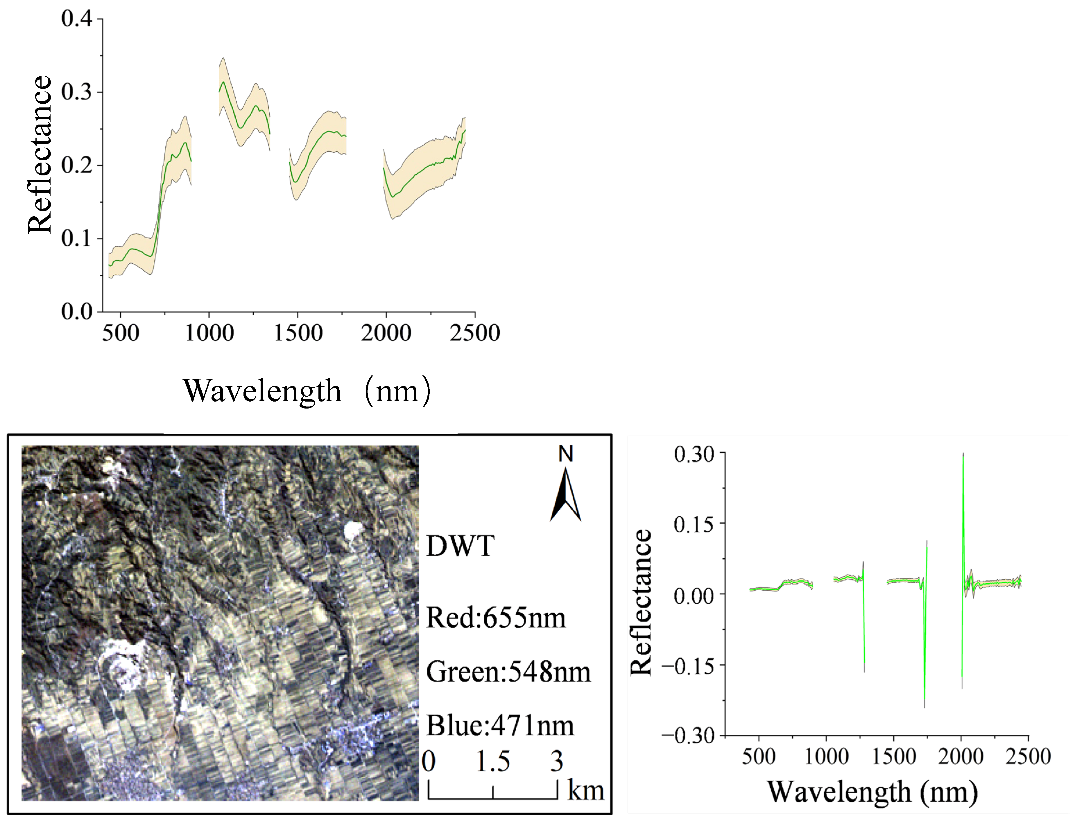
2.3. Satellite Hyperspectral Data Acquisition

The hyperspectral images of the region were acquired by the Advanced Hyperspectral Imager (AHSI) onboard the GF-5 satellite; the data were sourced from the China Land Observation Satellite Data Service Center (https://data.cresda.cn/#/2dMap, accessed on 26 August 2023). The AHSI data collected in November 2019, with a spatial resolution of 30 m and swath width of 60 km, was used for this study. After removing the overlapping bands and excluding the bands affected by low sensor signal-to-noise ratio (SNR), instrument artifacts, and strong atmospheric water-vapor absorption; we considered the spectral intervals of 430–900, 1050–1350, 1451–1771, and 1982–2450 nm (from a total of 330 bands, 240 bands were selected; spectral resolution = 5 or 10 nm). Radiometric calibration and atmospheric correction were performed using ENVI 5.5.

Fractional-order derivative (FOD) models can extract sensitive information from spectral data within a narrow order range and optimize the feature-band selection process [26]. Using a step-size of 0.2, the FOD was incrementally applied from order 0 to 2 to explore the optimal fractional derivative. Discrete wavelet transform (DWT) is widely used for processing the non-stationary signals in RS images [27]. In this study, the Bior 1.3 wavelet function was used for the wavelet decomposition of the hyperspectral data to remove high-frequency noise; this step was followed by wavelet reconstruction. These processes were implemented in MATLAB R2018b. Stable competitive adaptive reweighted sampling (SCARS) has been shown to be a superior feature-variable selection method for both linear and non-linear models [28]. Based on extensive preliminary experiments, in this study, the bands selected by the optimal FOD, DWT denoising, and SCARS methods were identified as the optimal GF-5 hyperspectral bands [29].

2.4. Extraction of Crop Phenology Data

In this study, we used the 44 HJ-1A/1B CCD images of the target region for 2020–2021, acquired from the China Centre for Resources Satellite Data and Application (CRESDA; https://data.cresda.cn/#/home, accessed on 26 August 2023). These images had a spatiotemporal resolution of 30 m [30] and a revisit cycle of 2 days. After image and radiometric calibration and atmospheric and geometric correction, the normalized difference vegetation index (NDVI) timeseries curves were calculated using the ENVI 5.3 software. Furthermore, Savitzky–Golay (S-G) filtering was applied for noise reduction and the reconstruction of crop growth curves. The crop phenological parameters were generated using the dynamic threshold method [31], wherein the start of the growing season (SOS) was defined as the date when the vegetation index increases beyond a specified fraction (threshold) of its seasonal amplitude (difference between the base level and the maximum value for the season); in this method, the end of the growing season (EOS) was defined on the right side of the fitted curve [7]. A threshold of 20% was set, and the phenological parameters were extracted using the TIMESAT 3 software.

2.5. Extraction of Cropping Index Data

From sowing to harvest, NDVI values depict dynamic increases/decreases corresponding to the crop phenology. Each peak in the NDVI timeseries represents the peak growth stage of a crop cycle. Furthermore, the number of peaks extracted from the NDVI timeseries determines the number of crops grown per year (cropping index). Based on the smoothed NDVI timeseries curve, the number of peaks was determined using the second derivative method [32]. In our study, the field surveys confirmed that all crops in the region had independent growth periods that exceeded 3 months; the interannual fluctuation in the heading stage was within 7 days, because of the variations in the hydrothermal conditions across the region. Note that crop NDVI typically peaks at the heading stage and reaches the minimum value before sowing or after harvest. To eliminate “false peaks” potentially identified by the second derivative method, in this study, we applied two rules: First, the interval between two NDVI peaks must be at least 3 months (equivalent to the 6 HJ-1A/1B NDVI values, as the images were captured roughly every 15 days). Second, the peak NDVI must be greater than 0.5, and the peak-to-trough difference must be greater than 0.1. This calculation was carried out using the ENVI 5.6 software. The number of peaks extracted based on these rules defined the cropping index [7], which varied from 0 to 3. Furthermore, we conducted field interviews with the local land users to verify the crop rotation pattern at each sampling point. Fallow farmland depicted a cropping index of 0, with single-, double-, and triple-cropping corresponding to indexes of 1, 2, and 3, respectively. The accuracy of the extracted crop rotation results was evaluated using a confusion matrix.

2.6. Selection of Environmental Covariates

In this study, we considered five categories of environmental variables, namely, topographic factors, soil properties, climatic variables, vegetation indices, and farmland management practices, as the auxiliary data required to support the satellite hyperspectral images for SOC-prediction and mapping.

The soil texture data (sand, clay) were derived from the World Soil Information Service (WoSIS) soil grid database provided by the International Soil Reference Information Centre (ISRIC; www.isric.org, accessed on 26 August 2024), with a resolution of 250 m × 250 m. The topographic factors (including slope and aspect, resolution of 30 m × 30 m) were generated from the digital elevation model (DEM); the DEM data were sourced from the United States Geological Survey (USGS; www.usgs.gov, accessed on 26 August 2023) (resolution of 30 m × 30 m). The climate factors were sourced from the Fine-Resolution Mapping of Mountain Environment (FRMM) project data; this included the data pertaining to temperature, precipitation, and actual evapotranspiration (at a resolution of 30 m × 30 m). The NDVI data (resolution of 30 m × 30 m) were sourced from the Data Registration and Publishing System of the Data Center for Resources and Environmental Sciences, Chinese Academy of Sciences. The net primary productivity (NPP) data (resolution of 250 km × 250 km) were sourced from the moderate resolution imaging spectroradiometer annual NPP product of the National Aeronautics and Space Administration (NASA; www.nasa.gov, accessed on 26 August 2023). The vegetation phenology parameters were extracted from the NDVI timeseries RS data. We selected two important parameters, SOS and EOS. The cropping index (CI) was calculated based on the peak characteristics of the NDVI timeseries curve. In 2020, based on the project of farmland quality update and evaluation, local farmers and staff from the soil and fertilizer station were interviewed; on-site investigations were conducted to record the irrigation (Irr) and drainage (Dra) capacities and the situation of farmland forest network. The data results were based on the basic unit of farmland patches, and the ArcGIS 10.8 polygon-to-raster tool was used to generate the raster data (with a resolution of 30 m × 30 m). The data of nitrogen fertilizer (NF) application rate (with a resolution of 5 km) were sourced from the National Ecological Data Center. The types and sources of each environmental variable are shown in

Table 1. Types and data sources of environment variables.

Environmental Category	Environmental Variable	Unit	Data Source
Topography	Slope	°	Derived from DEM data (30 m × 30 m)
	Aspect	°
Soil	Sand	%	ISRIC SoilGrids (1:1,000,000; 250 m × 250 m)
	Clay	%
Climate	Mean annual temperature (MAT)	°C	FRMM (30 m × 30 m)
	Mean annual precipitation (MAP)	mm
	Actual evapotranspiration (EVA)	mm
Vegetation	Normalized difference vegetation index (NDVI)	index values	Resource and Environment Data Center, CAS (30 m × 30 m)
	Net primary productivity (NPP)	gC·m−2	MODIS MOD17 Annual NPP Product, NASA (250 m × 250 m)
	Start of the growing season (SOS)	day	Extracted from NDVI timeseries remote sensing data
	End of the growing season (EOS)	day
Farmland Management	Irrigation capacity (Irr)	index values	Field surveys (2020); Rasterized in ArcGIS 10.8 (30 m × 30 m)
	Drainage capacity (Dra)	index values
	Nitrogen fertilizer application rate (NF)	gNm−2	National Ecological Data Center (resolution of 5 km)
	Cropping index (CI)	%	Identified via peak detection in NDVI time series curves

. To address the differences in coordinate reference systems and resolutions, all datasets were resampled to 30 m × 30 m raster data using the nearest-neighbor resampling method in ArcGIS 10.8, and the data were projected onto the WGS 84/World Mercator coordinate system.

2.7. Random Forest (RF) Modeling

Random forest (RF) is a widely used ensemble tree-based machine learning (ML) technique in DSM [33]; the model is known for its clarity, ease of interpretation, stability, resistance to overfitting, and tolerance to multicollinearity. In this study, the number of trees (num.trees) was set to 1000, and the number of variables tried at each split (mtry) was generally set to n/3 (with n denoting the number of predictors). Other parameters were set to the default values [29].

To investigate whether combining GF-5 satellite hyperspectral data with environmental variables improved the farmland SOC-prediction accuracy and to assess the influence of crop phenology and farmland management measures on the prediction accuracy of the model, four RF training models were constructed based on the optimal GF-5 satellite hyperspectral data model, while considering different environmental variable combinations: (1) RF-N: RF model using only natural variables (topography, soil, vegetation, and climate; excluding crop phenology SOS/EOS); (2) RF-P: RF model using natural variables including crop phenology (SOS, EOS); (3) RF-M: RF model using natural variables (excluding phenology) + farmland management factors; and (4) RF-A: RF model using all environmental variables (natural + phenology + farmland management). The data for all environmental variables at the soil sample points were extracted using ArcGIS 10.8 (ESRI, Inc., Redlands, CA, USA). The four RF models were used for the regression prediction of farmland SOC. Then, the trained models were applied to each pixel of the hyperspectral images to generate spatial distribution maps of farmland SOC across the study area. Model prediction accuracy was evaluated using the mean absolute error (MAE), root mean square error (RMSE), and coefficient of determination (R²). To assess the uncertainty of the farmland SOC maps, each RF model was run 100 times. For each grid cell, the mean and standard deviation (SD) of the 100 generated SOC maps were calculated to represent the predicted SOC value and the associated uncertainty [34]. Finally, the spatial distribution maps of farmland SOC and their uncertainty were produced using the mapping module in ArcGIS 10.8.

2.8. Random Forest (RF) Factorial Experiments

In general, RF models can assess variable importance, defined as the average contribution of each variable to the prediction across all trees; thus, they can be used to clarify the relative contributions of variables. In this study, we employed RF factorial experiments [35] using the full-variable RF model (while excluding satellite hyperspectral data) to distinguish the effects of topography (T), vegetation (V), climate (C), soil (S), and farmland management factors (M) on the farmland SOC in the study area. Six independent RF models were used: one model included all the drivers (hereinafter referred to as RF_all), and five models sequentially excluded topography (hereinafter referred to as RF_te), climate (hereinafter referred to as RF_clim), vegetation (hereinafter referred to as RF_vege), soil (hereinafter referred to as RF_soil), and farmland management (hereinafter referred to as RF_ma). First, the impact of a target driver category was isolated; then, its actual contribution, ActCon, was quantified by comparing the results of the above-mentioned models [Equation (1)]:

ActCon_V_j = RF_all − RF_V_j

(1)

where V_j represents the target driver category j, ActCon_V_j is the actual contribution of driver V_j, and RF_V_j is the regression result excluding driver V_j.

The relative contribution, RelCon_V_j, of driver category V_j was defined by Equation (2):

$$RelCon\_V_j = \left(\right|ActCon\_V_j\left|\right)/\left({\mathsf{\Sigma }}_j^n\right|ActCon\_V_j\left|\right) \times 100\%$$

(2)

Notably, the RF modeling and variable importance analysis were conducted using the Random Forest package in R 4.4 (R Core Team, 2016). The predictive mapping of the spatial distribution of SOC was performed using the mapping module in ArcGIS 10.5.

2.9. Partial Least Squares Structural Equation Modeling

Structural equation modeling (SEM) is an effective method for estimating and testing the causal relationships among variables; it can describe complex relationships among multiple latent variables [36]. In this study, path analysis was conducted to clearly elucidates the relationships and strengths of various indicators that influenced the target variable, while exploring the interrelationships among individual indicators. Furthermore, partial least squares structural equation modeling (PLS-SEM) was employed to assess the direct and indirect effects of various variable categories on the farmland SOC in the Yuncheng Basin in China.

3. Results

3.1. Mapping Soil Organic Carbon Using Satellite Hyperspectral and Environmental Variables

The descriptive statistics of the SOC content for the study region are presented in

Table 2. Descriptive statistics of soil organic carbon (SOC) content for the study region.

Number of Samples	Maximum (g/kg)	Minimum (g/kg)	Mean (g/kg)	Median (g/kg)	Standard Deviation (SD: g/kg)	CV (%)
312	19.20	1.42	9.96	9.82	2.98	29.92

. The SOC values for the 312 soil samples varied from 1.42 g/kg to 19.20 g/kg, with the mean being 9.96 g/kg, which was slightly higher than the median (9.82 g/kg). The SD was 2.98 g/kg, and the coefficient of variation (CV) was 29.92%, indicating moderate variability.

Through extensive experimentation, the RF model built using the feature bands selected by the 0.8 FOD-DWT-sCARS method significantly outperformed other prediction models, exhibiting a higher R² and lower RMSE and MAE values (R² = 0.69, RMSE = 1.58 g/kg, MAE = 0.64 g/kg); the results can be found in this paper [29]. Figure 3 presents a local satellite image processed using the 0.8 FOD-DWT method (the optimal denoising method) and its corresponding spectral reflectance plots. The green line represents the mean soil spectral signature, and the yellow area represents the SD. The 0.8 FOD-DWT processing amplified parts of the spectral curves, depicting the variations clearer and facilitating the differentiation between various SOC content levels. The spatial distribution of the topsoil SOC predicted by this model and the associated prediction uncertainty are shown in Figure 4a and Figure 4b, respectively. The mean predicted SOC value (10.28 g/kg) was close to the measured mean. However, the range, CV, and SD of the predicted values were significantly lower than those of the measured values (Figure 4a). These results were consistent with the SOC prediction presented in previous studies [37], indicating a stable model in terms of the simulation accuracy and the ability of the model to capture spatial heterogeneity.

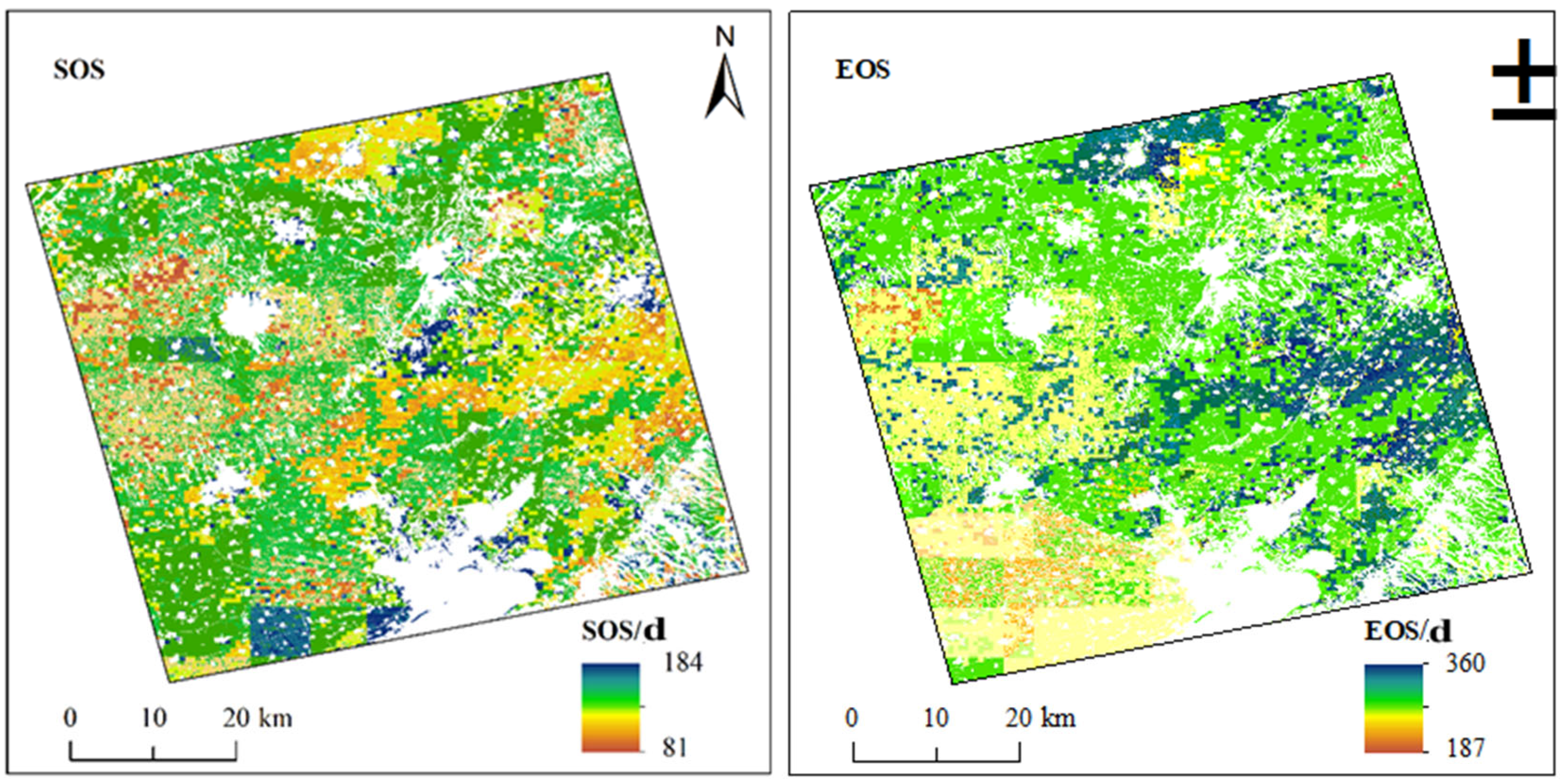
3.2. Spatial Distribution of Crop Phenology

The SG filter was applied to smooth, denoise, and reconstruct the NDVI timeseries curves for 2020–2021. Figure 5 presents an example of NDVI timeseries curves before and after SG filtering. Compared to the original curve, the smoothing process effectively removed the noise, while preserving the fundamental characteristics of the curve. It also enhanced the depiction of alternating peaks and valleys, effectively capturing the rhythmic pattern of crop growth; thus, this process was suitable for extracting the crop phenology and determining the subsequent CI. Figure 6 presents the spatial distribution maps of crop SOS and EOS. Due to the relatively small variations in the elevation and temperature differences across the study area, the phenological values showed limited spatial variation. The mean SOS occurred around day 120 of the year, with earlier values observed in parts of the central-eastern, north-central edge, and northwestern areas. The mean EOS occurred around day 310, with the later values observed in parts of the central-eastern region and the north-central edge. Furthermore, in the southwestern part of the study area, the SOS and EOS occurred relatively late and early, respectively, indicating a shorter phenological period for the crops in this region.

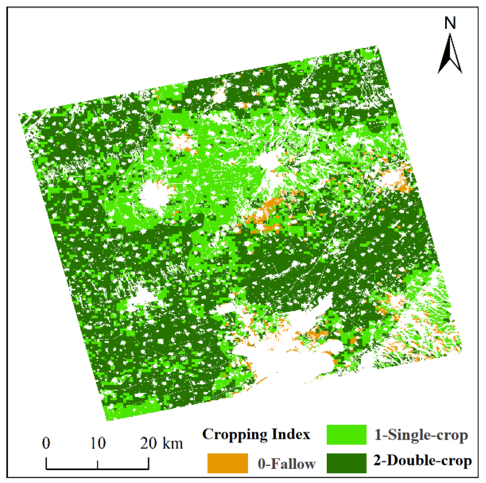
3.3. Spatial Distribution of Cropping Index (CI)

The distribution pattern of CI is generally shaped by natural factors and long-term cultivation practices, remaining relatively stable over short periods because of the dominant role of human control. Figure 7 presents the spatial distribution map of the CI for the study area for 2020–2021. Overall, double-cropping systems (CI = 2) were predominantly distributed in low-elevation plains; single-cropping systems (CI = 1) were concentrated in parts of the central-eastern and north-central edge regions; and fallow land (CI = 0) was sporadically distributed in high-altitude sloping farmland. Due to the constraints related to water, heat, and economic conditions, a triple-cropping system (CI = 3) was absent in the study area. The accuracy of the extracted CI was validated using the field survey results of all the 312 sample points (

Table 3. Confusion matrix for cropping index extracted from time-series NDVI data.

	Cropping Index			Producer’s Accuracy (%)
	Fallow	Single-Crop	Double-Crop
Fallow	19	4	1	79.16
Single-crop	2	75	6	90.36
Double-crop	4	10	192	93.20
User’s Accuracy (%)	76.00	84.26	96.48
Overall Accuracy: 88.77%; Kappa Coefficient: 0.8012

). Irrigated land in the study area predominantly supported a double-cropping pattern (rotation), while dryland mostly involved a single-cropping pattern (monoculture). The overall accuracy of the extracted CI was approximately 88.77%, with both single- and double-cropping patterns achieving accuracies above 80%.

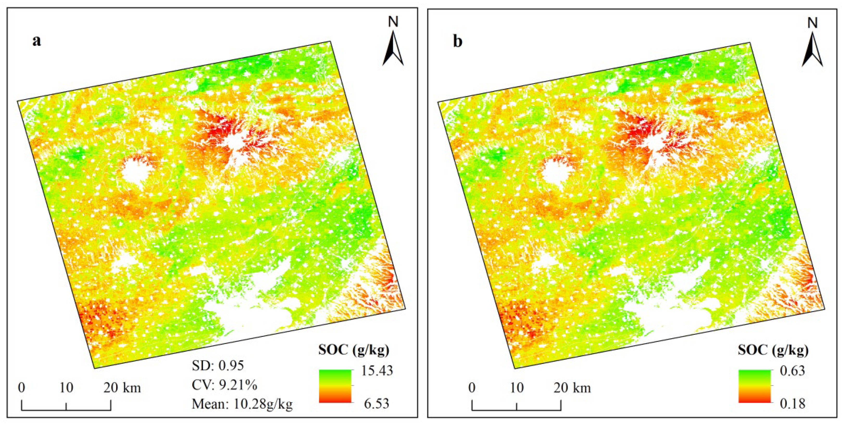
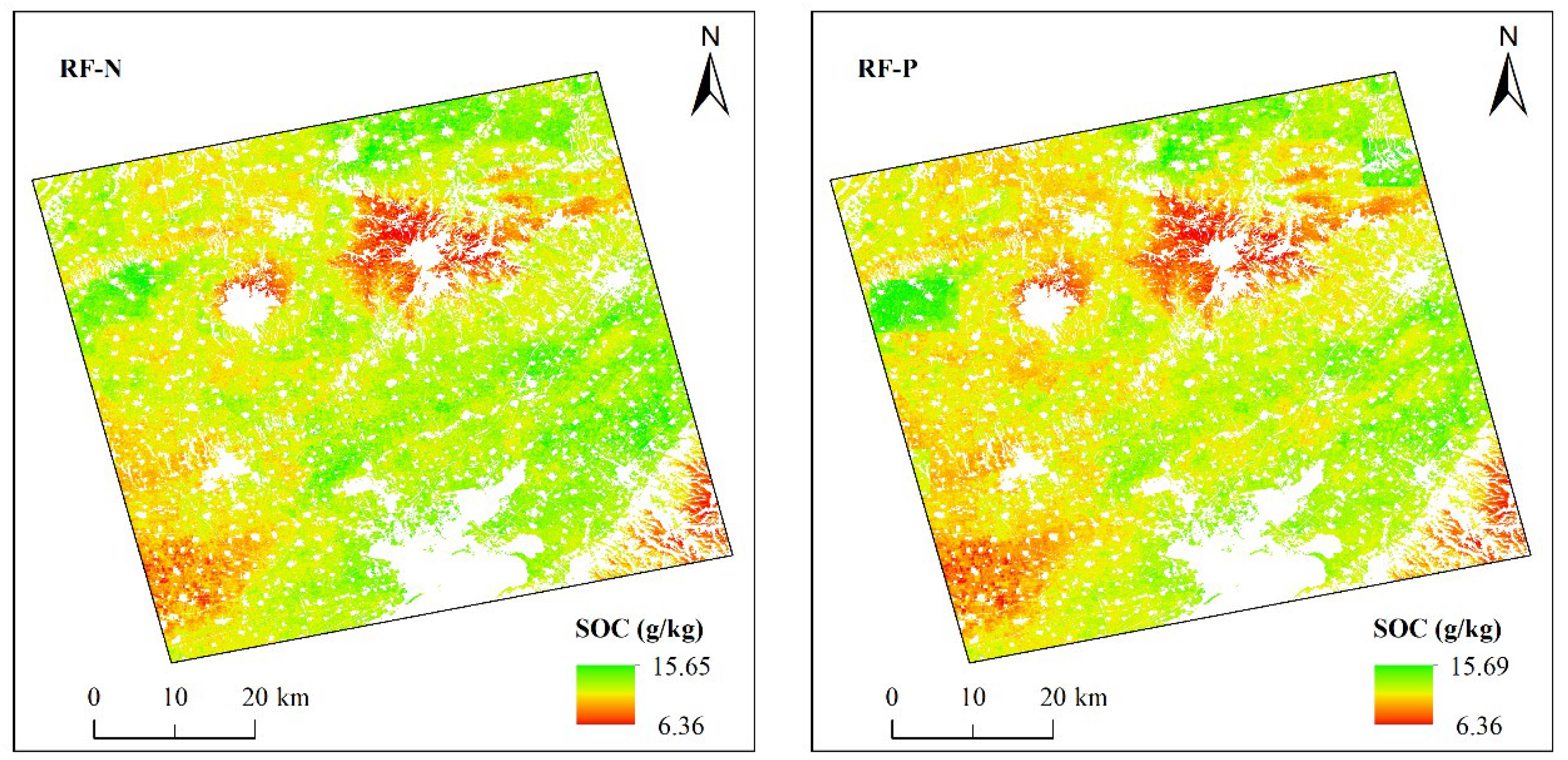
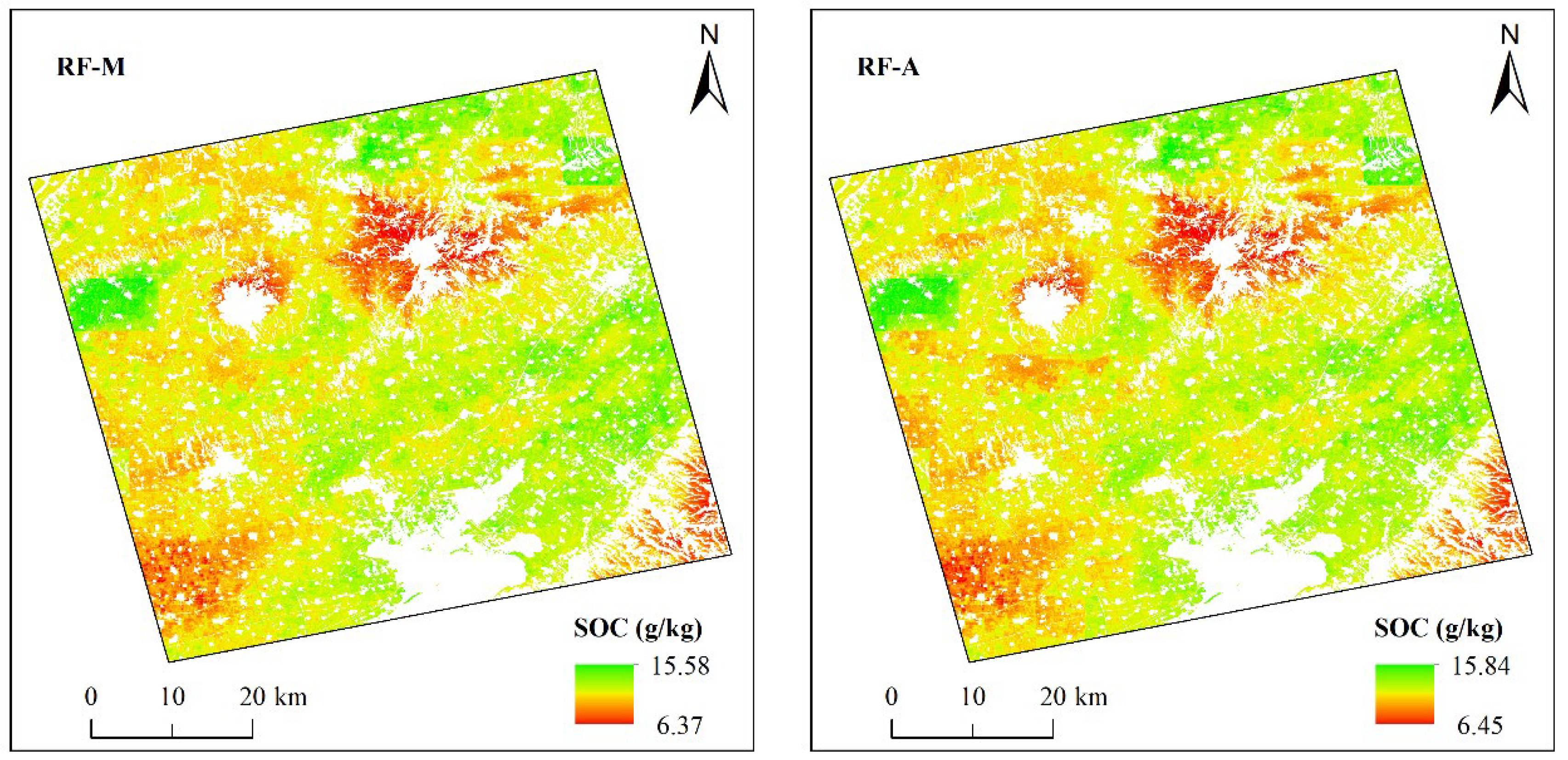
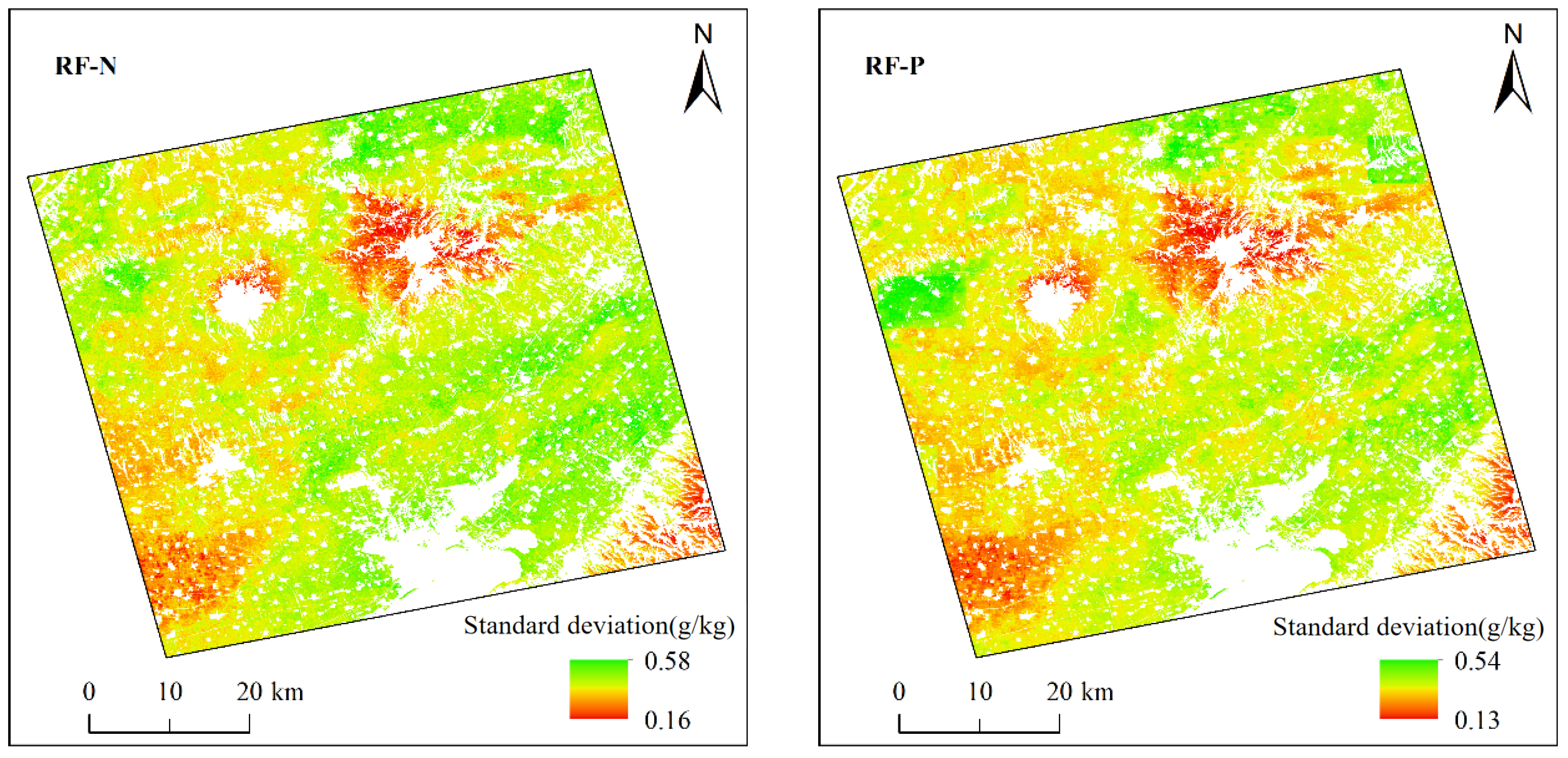
3.4. Spatial Distribution of Farmland Soil Organic Carbon

Compared to using the optimal satellite hyperspectral prediction model alone (0.8 FOD-DWT-sCARS: R² = 0.69, RMSE = 1.58 g/kg, MAE = 0.64 g/kg) [29], the introduction of environmental variables into the model significantly improved the prediction accuracy of farmland SOC (

Table 4. Predicted results of the four RF models under different variable combinations.

Model	Max (g/kg)	Min (g/kg)	Mean (g/kg)	SD (g/kg)	CV (%)	R2	RMSE (g/kg)	MAE (g/kg)
RF-N	15.65	6.36	10.35	0.97	9.37	0.78	1.40	0.52
RF-P	15.69	6.36	10.36	1.02	9.84	0.81	1.37	0.49
RF-M	15.78	6.37	10.13	1.02	10.07	0.87	1.22	0.43
RF-A	15.84	6.45	10.07	1.04	10.33	0.89	1.14	0.41

Note: RF-N: random forest model using only natural variables; RF-P: random forest model using natural variables and crop phenology; RF-M: random forest model using natural variables and farmland management; RF-A: random forest model using natural variables, crop phenology, and farmland management.

). The RF-N model showed significant improvement: the RMSE and MAE decreased, and the R² increased by 0.09. The prediction accuracy of the model increased with the introduction of crop phenology (RF-P) and farmland management factors (RF-M), with a further decrease in the RMSE and MAE and further increase in R². This indicates that the type of variables (different combinations of environmental variables) significantly affected the predictive performance for farmland SOC. The RF-A model achieved the lowest RMSE and MAE (RMSE = 1.14 g/kg, MAE = 0.41 g/kg) and the highest R² value (0.89), denoting an increase of 0.20 over the value observed when using the hyperspectral model alone. Therefore, the RF-A model was the most effective for predicting the spatial distribution of farmland SOC. The mean predicted SOC values from all four RF models were very close to the measured mean (approximately 10.00 g/kg). However, the range, CV, and SD of the predicted values were consistently lower than those of the measured values (Table 4), aligning with previous studies on farmland SOC prediction [37]. Notably, the range of SOC content predicted by the RF-A model was significantly larger than those predicted by the other three models, indicating that the model captured greater spatial variability, thereby affirming its superior simulation accuracy and enhanced ability to capture the spatial heterogeneity of the study region. Figure 8 presents the spatial distribution maps of the farmland SOC for the study region predicted using the four RF models. The areas with low SOC were primarily located in high-altitude mountainous regions, characterized by sloping farmland, fragmented plots, relatively low soil quality, and poor fertility. Overall, farmland SOC exhibited a trend of higher values in the east and lower values in the west. This pattern may be attributed to the proximity of the western areas to the Yellow River, resulting in higher sand content.

Each RF model was run 100 times, and the SD of the predictions was calculated to assess the uncertainty of the results (Figure 9). The results showed small SD values, varying between 0.08 g/kg and 0.58 g/kg, indicating good performance in estimating the farmland SOC across the study region. The RF-A model exhibited the smallest range of SD values, demonstrating that the model had the greatest stability in predicting the farmland SOC across the study region. Therefore, we could conclude that introducing crop phenology and farmland management factors, in addition to natural variables, effectively reduced the prediction uncertainty of the model. Notably, the spatial pattern of prediction uncertainty resembled the SOC distribution itself, with areas of higher SOC content also exhibiting higher uncertainty.

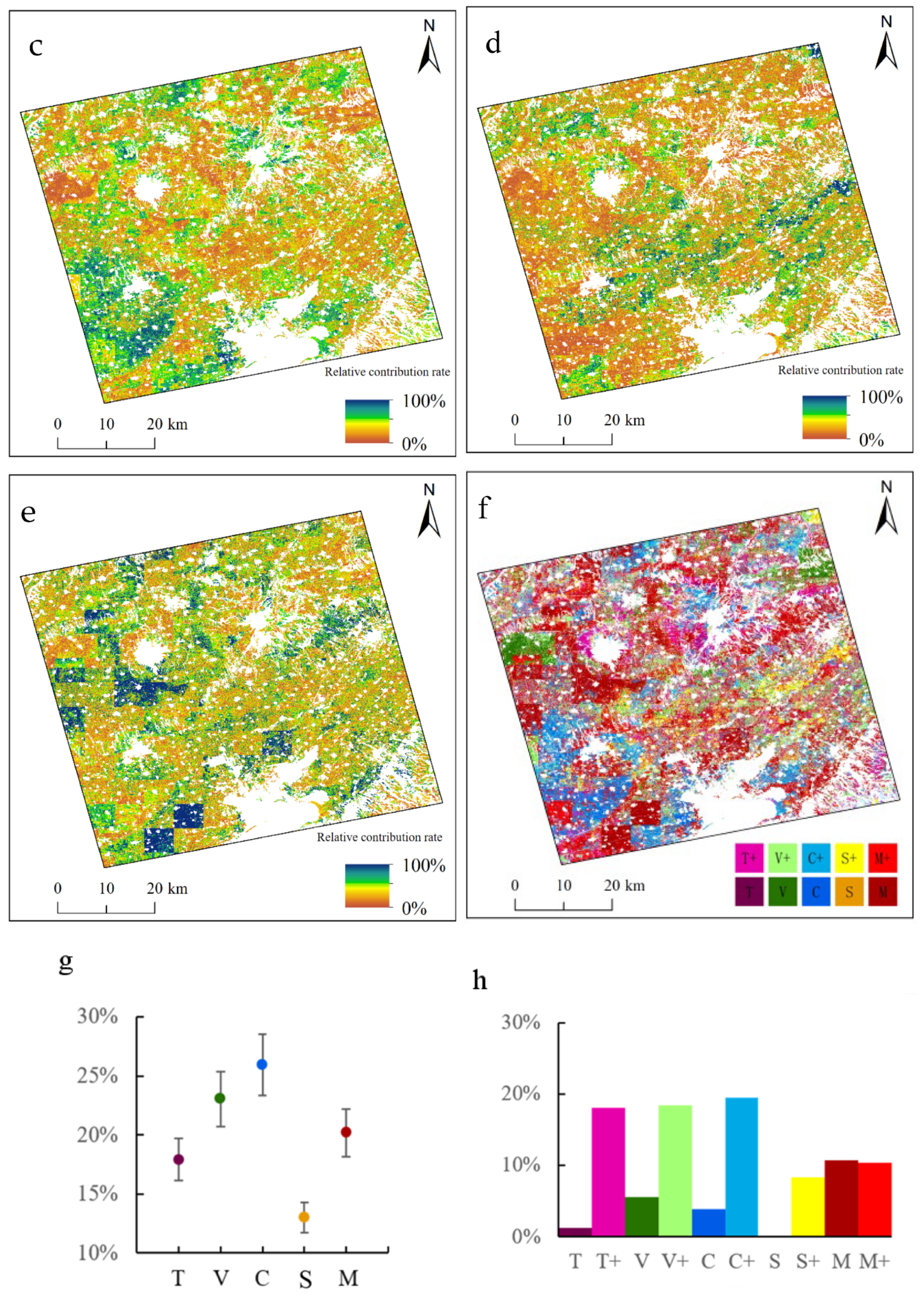
3.5. Relative Contribution of Environmental Variables

The relative contributions of the five environmental variable categories to the farmland SOC in the study region were visualized per pixel. Furthermore, the dominant driving category for each pixel was defined as the category with relative contribution greater than 60%. If the maximum relative contribution from any single category was below this threshold but fell within the 40–60% range, the dominant category for that pixel was defined as the combined effect of that and other categories. The relative contribution results are presented in Figure 10. Figure 10a–e represent the contribution rates of topography (T), vegetation (V), climate (C), soil (S), and farmland management (M) factors, respectively. Figure 10f presents the spatial distribution of the dominant controlling category. Figure 10g displays the average relative contribution of each category. Figure 10h illustrates the proportion of area driven by different categories and their combinations, with ‘+’ denoting the coupled effect of multiple categories.

The influence of topography, climate, soil, vegetation, and farmland management activities on the variations in the SOC differed across the spatial locations within the study area (Figure 10). Overall, the average influence degrees were as follows: topography (17.88%), vegetation (23.04%), climate (25.93%), soil (12.99%), and farmland management (20.16%) (Figure 10g). This indicates that climate was the most important driver of the spatial variability of SOC. The areas strongly influenced by climate were widely distributed in the western and southern parts of the study area (Figure 10c). The influences of vegetation and farmland management activities were also substantial. The vegetation-influenced areas were mainly concentrated in the northern region and parts of the central-eastern area (Figure 10b), while the farmland management-influenced areas were relatively dispersed, primarily located in the northwestern parts (Figure 10e). Note that the SOC was relatively less influenced by topography and soil, with their main influence zones being located in the high-altitude areas and parts of the central-eastern region, respectively (Figure 10a,d). Figure 10f shows the spatial distribution of the dominant driving factor interactions. The combined effect of climate and other factors was the most significant combination to influence the spatial variability of SOC (Figure 10f,h). The combined effects of topography and other factors and vegetation and other factors also had relatively large impacts on the SOC in the study area. Independent single drivers had limited influence on the spatial variability of SOC (Figure 10f). Among the single dominant factors, the influence of farmland management was the strongest. Moreover, the area dominated by farmland management alone or a combination of driving factors was relatively large, underscoring the significant impact of the driving factor. In the southern basin, farmland management coupled with other factors and climate coupled with other factors dominated the SOC variability. In high-altitude and western basin areas, topography and soil were the dominant driving factors. The coupled effect of vegetation and other factors was highly dispersed, mainly influencing parts of the central-eastern region. The prevalence of T+, V+, C+, S+, and M+ categories confirmed that the coupled effects of different driver categories dominated the spatial variability of farmland SOC across the study area.

3.6. Driving Factor Analysis of Farmland Soil Organic Carbon and Covariate Determination Using Structural Equation Modeling

To better assess the influence of individual environmental variables on the farmland SOC content across the study region, a PLS-SEM model was constructed. Various paths were built for all the factors, with respect to the five categories: farmland management (NF, CI, Irr, and Dra), topography (slope, aspect), vegetation (SOS, EOS, NPP, and NDVI), climate (MAT, MAP, and EVA), and soil (sand, clay). Based on the established soil science theory, the SEM paths were appropriately adjusted, resulting in a final model with good fit indexes (χ²/df = 1.129, CFI = 0.993; RMSEA = 0.056; SRMR = 0.06, R² = 0.56), explaining 56% of the SOC variation (Figure 11).

In Figure 11, single-headed arrows represent the assumed effect of one variable (cause) on another (outcome). Double-headed arrows represent the covariance/correlation (mutual influence). Solid arrows indicate the statistically significant paths (p < 0.05). Dashed arrows indicate the non-significant relationships (p > 0.05), straight lines (red) represent the direct effects, and curved lines (black) represent the indirect effects. Furthermore, the numbers on the arrows represent the standardized path coefficients. Note that the line thickness corresponds to the magnitude of the path coefficient. Sign +/− indicates the direction of the effect (positive/negative), and the larger absolute values signify stronger influence.

The SEM (Figure 11) revealed that NF was the most important factor to directly affect the farmland SOC in the study region (path coefficient = 0.31, p < 0.01). Among the farmland management factors, excluding NF (0.31), CU (0.29) and Irr (0.13) depicted significant direct positive effects on the farmland SOC across the region. Notably, the effect of Dra (0.09) was not significant. Among the vegetation factors, EOS (0.18), SOS (0.21), NPP (0.25), and NDVI (0.12) depicted significant positive effects on farmland SOC. Among the climate factors, MAT (−0.19), MAP (0.28), and EVA (−0.11) had significant effects on farmland SOC, with MAT and EVA depicting negative effects. Among the topographic factors, slope (−0.24) and aspect (0.14) depicted significant effects (p < 0.05), with slope exhibiting a negative effect. Among the soil factors, sand (−0.15) and clay (0.23) depicted significant effects (p < 0.05), with sand showing a negative effect.

Overall, all the five categories presented significant direct effects on the farmland SOC across the region (p < 0.05): farmland management (0.38), vegetation (0.31), climate (0.23), soil (0.22), and topography (−0.18). Overall, the topography category exhibited a negative net effect. Farmland management activities depicted the strongest overall influence on the SOC content variation across the region, followed by vegetation. Climate and soil factors exhibited roughly similar magnitudes of influence, while topography had a relatively smaller impact. Within farmland management, NF, CI, and Irr indirectly affected the SOC by influencing the soil physicochemical properties (0.14) and vegetation growth (0.12) in the region. Climate factors had a significant direct effect on the SOC variation (p < 0.05) and also interacted with vegetation change (0.19), indicating that climate indirectly affected the farmland SOC through its influence on vegetation growth. Topography factors indirectly affected the SOC variation across the region through their influence on vegetation growth (0.15) and further indirectly through climate (0.13) and farmland management (0.11). Farmland management (0.14), climate (0.08), vegetation (0.09), and topography (0.12) indirectly influenced the soil texture, moisture, and nutrient status, thereby indirectly affecting the farmland SOC content across the study region.

4. Discussion

4.1. Comparison of Digital Soil Mapping Models Employed for Assessing Farmland Soil Organic Carbon

In this study, we utilized optimally processed GF-5 satellite hyperspectral bands, various natural factors (soil, topography, climate, and vegetation), and farmland management factors (CI and phenology) as auxiliary variables within four RF models, to predict and map the spatial distribution of farmland SOC across the study area. Combining satellite hyperspectral data with environmental variables enhanced the farmland SOC prediction accuracy and confirmed the effectiveness of incorporating crop phenology and farmland management measures. Minor differences in the mapped SOC results may be attributed to the distribution and selection of training samples during modeling, leading to spatial prediction uncertainty. Therefore, we also evaluated the reliability of the mapping results by quantifying the uncertainty of the spatial distribution of the predicted SOC content.

The spatial distributions of the SOC predicted by the four RF models were similar, exhibiting strong spatial variability across all maps (Figure 8). Although the overall trends were comparable, the RF-A model depicted the best in capturing the spatial variability of farmland SOC, particularly in the western part of the study area. The analysis of the SOC map developed using the optimal RF-A model (Figure 8) revealed the highest predicted SOC values in parts of the central-eastern and north-central edge regions. These areas typically featured double-cropping (CI = 2) and long crop phenological periods. Frequent rotations over long growth cycles may facilitate greater crop straw incorporation, increasing the organic-matter input into the soil. Furthermore, tillage associated with each cropping cycle can stimulate soil microbial activity, enhancing the conversion of crop residues to organic carbon and promoting SOC accumulation [38]. The lowest SOC values were predicted for the farmlands located in the mountainous areas of the north-central basin and in the southeastern region. This may be primarily attributed to the high-altitude areas being sloping farmlands with poor accessibility, limited irrigation/drainage capacity, lower fertilizer application, and suboptimal crop growth, leading to reduced SOC inputs. Additionally, the farmland SOC content was relatively low in the western region, especially in the southwest (close to the Yellow River). Strong variations in the soil or geological structures observed in these regions may severely disrupt the soil microbial environment in the basin, hindering the storage and transformation of SOC, ultimately reducing the soil carbon stocks in the region. The remaining areas (single-cropping and fallow land) exhibited moderate SOC levels. These findings align with the results of previous studies on the spatial differentiation of farmland SOC content in the sediment deposition areas of the Yellow River Basin [39,40].

4.2. Influence of Environmental Variables on Farmland Soil Organic Carbon (SOC) Mapping

Building upon traditional natural variables and optimal satellite hyperspectral data processing, in this study, we further incorporated farmland management factors, such as crop phenology and CI, into the RF model. The resulting RF-A model achieved the best performance in predicting the spatial variability of farmland SOC in the study region. Our results demonstrate that adding phenology and farmland management to natural variables (RF-N), in conjunction with the use of soil hyperspectral information, increased the prediction accuracy of the model (R²) by 11% and reduced the RMSE and MAE by 26 and 11%, respectively (Table 4). Therefore, comprehensively considering soil hyperspectral information and natural and farmland management environmental variables significantly enhanced the prediction of farmland SOC and the mapping accuracy of the model. Consistent with our findings, Yang et al. [41] revealed that crop rotations extracted from NDVI timeseries data improved the prediction accuracy for farmland SOC. Tian et al. [6] reported that combining mining area farmland damage, crop rotation, and natural variables yielded the highest accuracy for predicting the SOC for mining-affected farmlands, confirming the effectiveness of crop rotation and phenology information in improving the model accuracy.

Although we did not compare the RF model with other prediction methods, previous studies suggest that RF outperforms the ordinary kriging (OK) [42] and support vector machine (SVM) models [43] for SOC prediction. However, a few studies indicated that multiple linear regression (MLR) and SVM could outperform RF [44], possibly because RF regression tends to over-smoothen the predictions beyond the training data range and could be prone to overfitting in the case of noisy classification or regression tasks. A systematic review by Pouladi et al. [45] presents an assessment of 217 selected papers (2010–2023) on SOC digital mapping, while considering RS-identified RF as the most frequently studied algorithm in DSM.

4.3. Direct and Indirect Effects of Environmental Variables on Farmland Soil Organic Carbon

RF offers higher site-specific accuracy but limited transferability, and SEM yields slightly lower explanatory power but better generalizability and mechanistic insight. Vegetation is a major source of SOC. Our study shows that crop rotation (CI = 2) derived from NDVI timeseries curves is crucial for improving the model prediction of farmland SOC. Furthermore, we could conclude that NPP, SOS, and EOS were among the most influential natural variables for SOC content prediction. In northern regions in China, in farmland management, crop straw is a significant source of SOC replenishment [15]; NPP can indirectly reflect the amount of straw available for incorporation, while SOS and EOS reflect the duration of the presence of crop residue.

Climate influences the soil moisture and temperature, groundwater level, and vegetation transpiration in a region. Heat and moisture conditions directly affect vegetation formation and distribution. Furthermore, climate variables also impact microbial activity and soil enzyme function, which are critical for soil carbon storage. In our work, MAT, MAP, and EVA were the main climate variables to influence the farmland SOC distribution across the study region and explain the spatial variation in the SOC. In large low-altitude farmland areas, relatively high MAT during the main summer growing season results in an increase in evaporation, thereby reducing water availability for crops and soil, potentially leading to lower SOC. The close relationship between MAP and soil moisture promotes plant growth [46], thereby corroborating our findings. Hobley et al. [47] also emphasized the importance of climate variables in SOC prediction.

Notably, topographic factors are closely related to SOC and also influence the soil texture at the regional scale [48]. In our study, slope showed relatively high importance for SOC prediction; in general, it affects the distribution of water and heat, further influencing the decomposition and transformation of SOC. Topographic factors, such as slope and aspect, are key determinants of soil formation processes. They affect soil development by altering parent material, soil moisture, and temperature conditions, and influence the spatial distribution of soil properties by controlling the flow of solutes, water, and sediments. Steeper slopes are generally less conducive to SOC formation. Previous SOC studies also identified slope and aspect as the key factors to influence the spatial distribution of farmland SOC content [7]. In hilly and mountainous areas, topography is often the dominant control for farmland SOC, but its influence may be diminished in plains [15].

Furthermore, the proportion of sand and clay in soil determines the soil structure, affecting the soil’s ability to retain water and nutrients and maintain permeability (aeration) and fertility. This significantly influences the quantity and quality of SOC, impacting its distribution. Furthermore, climatic temperature and soil texture composition influence the soil temperature. Changes in the soil temperature affect microbial activity and respiration rates, thereby governing the mineralization and decomposition processes of SOC [49].

Among farmland management factors, NF can regulate the soil carbon-to-nitrogen (C:N) ratio. Nitrogen content is crucial for soil carbon cycling, with studies suggesting that higher C:N ratios favor the accumulation of organic carbon [50]. Nitrogen fertilizers enhance soil fertility, promote crop growth, and increase plant productivity. In this study, fallow (CI = 0) and single-cropping farmlands (CI = 1) depicted slightly lower SOC content than double-cropping farmlands (CI = 2). Therefore, crop rotation in irrigated land appeared more conducive to SOC accumulation than monoculture in dryland. Consistent with our results, Tian et al. [7]. suggest that frequent rotations allow more straw to be returned to the field and more organic matter to enter the soil. Tillage stimulates microbial activity, enhancing the conversion of crop residues to organic carbon and promoting accumulation [51]. However, some studies indicate that dryland crop rotation can be detrimental to SOC accumulation [15], possibly because of increased tillage intensity and soil exposure, accelerating the breakdown of soil macroaggregates and raising SOC mineralization rates. Therefore, appropriate multiple cropping systems can increase or maintain SOC quantity and quality, thereby improving the chemical and physical properties of soil [52]. The intensity and duration of cultivation, coupled with the intensity of human management activities (e.g., irrigation and drainage capacity), are also key factors that influence the variations in SOC [53]. Integrating these factors can provide a better explanation for the SOC variations in plain areas and further improve the prediction accuracy of RF models.

5. Conclusions

In this study, we conducted fine-resolution mapping of the variations in farmland SOC variations in the Yuncheng Basin along the Yellow River in China by combining satellite hyperspectral data with various combinations of environmental variables. The major conclusions of this study are presented below: (1) The RF model that combined satellite hyperspectral data and 15 environmental variables achieved the highest prediction accuracy, captured the greatest SOC spatial variability, exhibited minimal uncertainty, and effectively delineated the spatial heterogeneity of SOC across the region. (2) Random forest (RF) factorial experiments provided the spatial estimates of the relative contributions and dominant driving categories of five environmental variable types, revealing their spatial influences on the SOC variation across the basin. Climate was the most important driver of the spatial variability of farmland SOC, and the climate-dominated areas were widely distributed in the southwestern part of the study area. (3) SEM elucidated the direct and indirect influence paths among the five major environmental categories and their factors. Farmland management activities had the strongest overall influence on the SOC variation across the study area, followed by vegetation. Climate and soil factors had roughly similar impacts, while topography had a relatively smaller influence.

Overall, this study provides precise farmland carbon sink data for the Yellow River Basin, supporting ecological zoning protection and promoting agricultural green transformation. Future studies should integrate the data from China’s Third National Soil Survey and incorporate the soil chemical and microbial indicators (which significantly influence the dynamic cycling and accumulation of SOC), while further exploring RS-based farmland management data and refining the methods used for soil attribute mapping at the regional scale.

References

1. McBratney, A.B.; Stockmann, U.; Angers, D.A.; Minasny, B.; Field, D.J. Challenges for soil organic carbon research. In Soil Carbon; Springer: Cham, Switzerland, 2014; pp. 3–16. [Google Scholar]
2. Jenny, H. Factors of Soil Formation: A System of Quantitative Pedology; McGraw-Hill: New York, NY, USA, 1941. [Google Scholar]
3. McBratney, A.B.; Santos, M.L.M.; Minasny, B. On digital soil mapping. Geoderma 2003, 117, 3–52. [Google Scholar] [CrossRef]
4. Mirzaee, S.; Ghorbani-Dashtaki, S.; Mohammadi, J.; Asadi, H.; Asadzadeh, F. Spatial variability of soil organic matter using remote sensing data. Catena 2016, 145, 118–127. [Google Scholar] [CrossRef]
5. Viscarra Rossel, R.A.; Webster, R.; Bui, E.N.; Baldock, J.A. Baseline map of organic carbon in Australian soil to support national carbon accounting and monitoring under climate change. Glob. Change Biol. 2014, 20, 2953–2970. [Google Scholar] [CrossRef]
6. Mulder, V.L.; Lacoste, M.; Richer-de-Forges, A.C.; Arrouays, D. GlobalSoilMap France: High-resolution spatial modelling the soils of France up to two meter depth. Sci. Total Environ. 2016, 573, 1352–1369. [Google Scholar] [CrossRef]
7. Tian, H.; Zhang, J.; Zheng, Y.; Shi, J.; Qin, J.; Ren, X.; Bi, R. Prediction of soil organic carbon in mining areas. Catena 2022, 215, 106311. [Google Scholar] [CrossRef]
8. Chen, S.; Liang, Z.; Webster, R.; Zhang, G.; Zhou, Y.; Teng, H.; Hu, B.; Arrouays, D.; Shi, Z. A high-resolution map of soil pH in China made by hybrid modelling of sparse soil data and environmental covariates and its implications for pollution. Sci. Total Environ. 2019, 655, 273–283. [Google Scholar] [CrossRef] [PubMed]
9. Liang, Z.; Chen, S.; Yang, Y.; Zhao, R.; Shi, Z.; Viscarra Rossel, R.A. National digital soil map of organic matter in topsoil and its associated uncertainty in 1980’s China. Geoderma 2019, 335, 47–56. [Google Scholar] [CrossRef]
10. Xu, D. Rapid Acquisition of Soil Information and Management Zones Delineation Based on Multi-Source Data Fusion at Field Scale. Ph.D. Thesis, Zhejiang University, Hangzhou, China, 2020. [Google Scholar]
11. Abbas, F.; Hammad, H.M.; Ishaq, W.; Farooque, A.A.; Bakhat, H.F.; Zia, Z.; Fahad, S.; Farhad, W.; Cerdà, A. A review of soil carbon dynamics resulting from agricultural practices. J. Environ. Manag. 2020, 268, 110319. [Google Scholar] [CrossRef]
12. Yang, L.; Cai, Y.; Zhang, L.; Guo, M.; Li, A.; Zhou, C. A deep learning method to predict soil organic carbon content at a regional scale using satellite-based phenology variables. Int. J. Appl. Earth Obs. Geoinform. 2021, 102, 102428. [Google Scholar] [CrossRef]
13. Kumar, N.; Nath, C.P.; Das, K.; Hazra, K.K.; Venkatesh, M.S.; Singh, M.K.; Singh, S.S.; Praharaj, C.S.; Sen, S.; Singh, N.P. Combining soil carbon storage and crop productivity in partial conservation agriculture of rice-based cropping systems in the Indo-Gangetic Plains. Soil Tillage Res. 2024, 239, 106029. [Google Scholar] [CrossRef]
14. Weiss, M.; Jacob, F.; Duveiller, G. Remote sensing for agricultural applications: A meta-review. Remote Sens. Environ. 2020, 236, 111402. [Google Scholar] [CrossRef]
15. Wu, Z. Research on Spatial Variation and Mechanism of Farmland Soil Organic Carbon in Plains. Ph.D. Thesis, Wuhan University, Wuhan, China, 2022. [Google Scholar]
16. Wang, R.; Du, W.; Li, P.; Yao, Z.; Tian, H. High-resolution mapping of cropland soil organic carbon in Northern China. Agronomy 2025, 15, 359. [Google Scholar] [CrossRef]
17. Kalaiselvi, B.; Chakraborty, R.; Dharumarajan, S.; Kumar, K.S.A.; Hegde, R. Spatial prediction of soil organic carbon and its stocks using digital soil mapping approach. In Remote Sensing of Soils; Elsevier: Amsterdam, The Netherlands, 2024; pp. 411–428. [Google Scholar]
18. Liu, S.; Chen, J.; Guo, L.; Wang, J.; Zhou, Z.; Luo, J.; Yang, R. Prediction of soil organic carbon in soil profiles based on visible–near-infrared hyperspectral imaging spectroscopy. Soil Tillage Res. 2023, 232, 105736. [Google Scholar] [CrossRef]
19. Ben-Dor, E.; Banin, A. Near-infrared analysis as a rapid method to simultaneously evaluate several soil properties. Soil Sci. Soc. Am. J. 1995, 59, 364–372. [Google Scholar] [CrossRef]
20. Dotto, A.C.; Dalmolin, R.S.D.; ten Caten, A.; Grunwald, S. A systematic study on the application of scatter-corrective and spectral-derivative preprocessing for multivariate prediction of soil organic carbon by Vis-NIR spectra. Geoderma 2018, 314, 262–274. [Google Scholar] [CrossRef]
21. Guo, L.; Zhang, H.; Shi, T.; Chen, Y.; Jiang, Q.; Linderman, M. Prediction of soil organic carbon stock by laboratory spectral data and airborne hyperspectral images. Geoderma 2019, 337, 32–41. [Google Scholar] [CrossRef]
22. Zhao, X.; Zhao, D.; Wang, J.; Triantafilis, J. Soil organic carbon (SOC) prediction in Australian sugarcane fields using Vis–NIR spectroscopy with different model setting approaches. Geoderma Reg. 2022, 30, e00566. [Google Scholar] [CrossRef]
23. Zhang, C.; Li, H.F.; Shen, H.F. Thin–cloud correction of GF–5 AHSI visible–light images by combining statistical information and scattering model. J. Remote Sens. 2020, 24, 368–378. [Google Scholar]
24. IUSS Working Group WRB. World Reference Base for Soil Resources 2014, Update 2015; World Soil Resources Reports No. 106; FAO: Rome, Italy, 2015. [Google Scholar]
25. Zhang, F.; Zhang, G. Chinese Soil Series: Central and Western Volume, Shanxi Volume; Longmen Books: Beijing, China, 2021. [Google Scholar]
26. Hong, Y.; Guo, L.; Chen, S.; Linderman, M.; Mouazen, A.M.; Yu, L.; Chen, Y.; Liu, Y.; Liu, Y.; Cheng, H.; et al. Exploring the potential of airborne hyperspectral image for estimating topsoil organic carbon: Effects of fractional-order derivative and optimal band combination algorithm. Geoderma 2020, 365, 114228. [Google Scholar] [CrossRef]
27. Meng, X.; Bao, Y.; Liu, J.; Liu, H.; Zhang, X.; Zhang, Y.; Wang, P.; Tang, H.; Kong, F. Regional soil organic carbon prediction model based on a discrete wavelet analysis of hyperspectral satellite data. Int. J. Appl. Earth Obs. Geoinform. 2020, 89, 102111. [Google Scholar] [CrossRef]
28. Li, G.; Gao, X.; Xiao, N.; Xiao, Y. Estimation Soil Organic Matter Contents with Hyperspectra Based on sCARS and RF Algorithms. Chin. J. Lumin. 2019, 40, 1030–1039. [Google Scholar]
29. Jin, H.; Peng, J.; Bi, R.; Tian, H.; Zhu, H.; Ding, H. Comparing laboratory and satellite hyperspectral predictions of soil organic carbon in farmland. Agronomy 2024, 14, 175. [Google Scholar] [CrossRef]
30. Wu, Z.; Liu, Y.; Han, Y.; Zhou, J.; Liu, J.; Wu, J. Mapping farmland soil organic carbon density in plains with combined cropping system extracted from NDVI time-series data. Sci. Total Environ. 2021, 754, 142120. [Google Scholar] [CrossRef]
31. Yang, L.; He, X.; Shen, F.; Zhou, C.; Zhu, A.; Gao, B.; Chen, Z.; Li, M. Improving prediction of soil organic carbon content in croplands using phenological parameters extracted from NDVI time series data. Soil Tillage Res. 2020, 196, 104465. [Google Scholar] [CrossRef]
32. Cui, J.; Song, D.; Dai, X.; Xu, X.; He, P.; Wang, X.; Liang, G.; Zhou, W.; Zhu, P. Effects of long-term cropping regimes on SOC stability, soil microbial community and enzyme activities in the Mollisol region of Northeast China. Appl. Soil Ecol. 2021, 164, 103941. [Google Scholar] [CrossRef]
33. Takoutsing, B.; Heuvelink, G.B.M. Comparing the prediction performance, uncertainty quantification and extrapolation potential of regression kriging and random forest while accounting for soil measurement errors. Geoderma 2022, 428, 116192. [Google Scholar] [CrossRef]
34. He, X.; Yang, L.; Li, A.; Zhang, L.; Shen, F.; Cai, Y.; Zhou, C. Soil organic carbon prediction using phenological parameters and remote sensing variables generated from Sentinel-2 images. Catena 2021, 205, 105442. [Google Scholar] [CrossRef]
35. Were, K.; Bui, D.T.; Dick, Ø.B.; Singh, B.R. A comparative assessment of support vector regression, artificial neural networks, and random forests for predicting and mapping soil organic carbon stocks across an Afromontane landscape. Ecol. Indic. 2015, 52, 394–403. [Google Scholar] [CrossRef]
36. Mousavi, S.R.; Sarmadian, F.; Angelini, M.E.; Bogaert, P.; Omid, M. Cause-effect relationships using structural equation modeling for soil properties in arid and semi-arid regions. Catena 2023, 232, 107392. [Google Scholar] [CrossRef]
37. Adhikari, K.; Hartemink, A.E. Digital mapping of topsoil carbon content and changes in the Driftless Area of Wisconsin, USA. Soil Sci. Soc. Am. J. 2015, 79, 155–164. [Google Scholar] [CrossRef]
38. King, A.E.; Blesh, J. Crop rotations for increased soil carbon: Perenniality as a guiding principle. Ecol. Appl. 2018, 28, 249–261. [Google Scholar] [CrossRef]
39. Feng, X.; Zhao, X.; Liu, Z.; Zhang, Y.; Gu, Q.; Zhang, J.; Guo, E. Distribution characteristics and influencing factors of soil organic carbon in the riparian zone of Mengjin Section of the Yellow River. J. Henan Agric. Univ. 2024, 58, 635–643. [Google Scholar]
40. Shi, J. Characteristics and Driving Mechanism of Soil Organic Carbon Stability in Typical Land Use Types in the Lower Yellow River Alluvial/Sedimentary Areas. Master’s Thesis, Henan University, Kaifeng, China, 2023. [Google Scholar]
41. Yang, L.; Song, M.; Zhu, A.; Qin, C.; Zhou, C.; Qi, F.; Li, X.; Chen, Z.; Gao, B. Predicting soil organic carbon content in croplands using crop rotation and Fourier transform decomposed variables. Geoderma 2019, 340, 289–302. [Google Scholar] [CrossRef]
42. Silatsa, F.B.T.; Yemefack, M.; Tabi, F.O.; Heuvelink, G.B.M.; Leenaars, J.G.B. Assessing countrywide soil organic carbon stock using hybrid machine learning modelling and legacy soil data in Cameroon. Geoderma 2020, 367, 114260. [Google Scholar] [CrossRef]
43. Forkuor, G.; Hounkpatin, O.K.L.; Welp, G.; Thiel, M. High resolution mapping of soil properties using remote sensing variables in south-western Burkina Faso: A comparison of machine learning and multiple linear regression models. PLoS ONE 2017, 12, e0170478. [Google Scholar] [CrossRef]
44. Moura-Bueno, J.M.; Dalmolin, R.S.D.; Ten Caten, A.; Dotto, A.C.; Demattê, J.A.M. Stratification of a local VIS-NIR-SWIR spectral library by homogeneity criteria yields more accurate soil organic carbon predictions. Geoderma 2019, 337, 565–581. [Google Scholar] [CrossRef]
45. Pouladi, N.; Gholizadeh, A.; Khosravi, V.; Borůvka, L. Digital mapping of soil organic carbon using remote sensing data: A systematic review. Catena 2023, 232, 107409. [Google Scholar] [CrossRef]
46. Wang, B.; Waters, C.; Orgill, S.; Gray, J.; Cowie, A.; Clark, A.; Liu, D.L. High-resolution mapping of soil organic carbon stocks using remote sensing variables in the semi-arid rangelands of eastern Australia. Sci. Total Environ. 2018, 630, 367–378. [Google Scholar] [CrossRef] [PubMed]
47. Hobley, E.; Wilson, B.; Wilkie, A.; Gray, J.; Koen, T. Drivers of soil organic carbon storage and vertical distribution in Eastern Australia. Plant Soil 2015, 390, 111–127. [Google Scholar] [CrossRef]
48. Zhu, H.; Bi, R.; Duan, Y.; Xu, Z. Scale-location specific relations between soil nutrients and topographic factors in the Fen River Basin, Chinese Loess Plateau. Front. Earth Sci. 2017, 11, 397–406. [Google Scholar] [CrossRef]
49. Wu, J.; Pan, J.; Ge, X.; Wang, H.; Yu, W.; Li, B. Variations of soil organic carbon mineralization and temperature sensitivity under different land use type. J. Soil Water Conserv. 2015, 29, 130–135. [Google Scholar]
50. Tian, H.; Liu, S.; Zhu, W.; Zhang, J.; Zheng, Y.; Shi, J.; Bi, R. Deciphering the drivers of net primary productivity of vegetation in mining areas. Remote Sens. 2022, 14, 4177. [Google Scholar] [CrossRef]
51. Jing, Y.; Bi, R.; Sun, W.; Zhu, H.; Ding, H.; Jin, H. Whether wheat-maize rotation influenced the change of soil organic carbon in Sushui River Basin. Land 2024, 13, 859. [Google Scholar] [CrossRef]
52. Giacometti, C.; Mazzon, M.; Cavani, L.; Triberti, L.; Baldoni, G.; Ciavatta, C.; Marzadori, C. Rotation and fertilization effects on soil quality and yields in a long term field experiment. Agronomy 2021, 11, 636. [Google Scholar] [CrossRef]
53. Sena, K.L.; Yeager, K.M.; Barton, C.D.; Lhotka, J.M.; Bond, W.E.; Schindler, K.J. Development of mine soils in a chronosequence of forestry-reclaimed sites in eastern Kentucky. Minerals 2021, 11, 422. [Google Scholar] [CrossRef]
Figure 1. Location of sampling area and the distribution of sampling points across the study area.
Agronomy 15 01827 g001
Figure 2. GF-5 satellite image captured during the sampling period.
Agronomy 15 01827 g002
Figure 3. Partial image and spectral reflectance of Goefen 5 (GF-5) satellite data processed using the 0.8 FOD-DWT method. The middle line represents the average value of soil spectral characteristics, while the lines at the top and bottom indicate the upper and lower boundaries of spectral standard deviation. The shaded area represents the standard deviation of the spectrum.
Agronomy 15 01827 g003
Figure 4. (a) Spatial distribution map and (b) uncertainty map of SOC in the study area predicted by the optimal hyperspectral model.
Agronomy 15 01827 g004
Figure 5. Comparison of representative NDVI timing curves before and after S-G filtering.
Agronomy 15 01827 g005
Figure 6. Spatial distribution of the start of season (SOS) and end of season (EOS).
Agronomy 15 01827 g006
Figure 7. Spatial distribution of the cropping index (CI).
Agronomy 15 01827 g007
Figure 8. Predicted spatial distributions of SOC by RF-N, RF-P, RF-M, and RF-A in the farmland.
Agronomy 15 01827 g008aAgronomy 15 01827 g008b
Figure 9. Uncertainty maps of farmland SOC predicted by the RF-N, RF-P, RF-M, and RF-A models.
Agronomy 15 01827 g009aAgronomy 15 01827 g009b
Figure 10. Relative contribution of the five environmental variable categories considered in this study. (ae) Spatial maps of contribution rates for topography (T), vegetation (V), climate (C), soil (S), and farmland management (M), respectively. (f) Spatial map of the dominant driving category. (g) Bar chart of average relative contribution per category. (h) Pie chart showing the proportional area driven by each category alone or in dominant combination (T+, V+, C+, S+, and M+ indicate the dominant coupling involving that category).
Agronomy 15 01827 g010aAgronomy 15 01827 g010b
Figure 11. Structural equation model (SEM) depicting the relationships between SOC and various environmental variables. Abbreviations: cropping index (CI), nitrogen fertilizer application rate (NF), irrigation capacity (Irr), drainage capacity (Dra), mean annual temperature (MAT), mean annual precipitation (MAP), actual evapotranspiration (EVA), start of season (SOS), end of season (EOS). * Indicates a significant correlation (p < 0.05), ** Indicates an extremely significant correlation (p < 0.01).
Agronomy 15 01827 g011