1. Introduction
In precision agriculture, detecting weeds and creating a weed pressure map is crucial for the effective use of variable-rate weeding equipment such as row cultivators, ground sprayers, or drones. The use of aerial image analysis to generate weed pressure maps and variable-rate intervention zones exemplifies how precision agriculture technologies can enhance input efficiency while minimizing environmental impact, directly supporting the United Nations’ Sustainable Development Goals—especially SDG 12 (Responsible Consumption and Production) and SDG 13 (Climate Action).
Wireless sensor networks, UAVs, and AI-based systems play a pivotal role in enabling real-time monitoring of field conditions and facilitating localized decision-making. These technologies help reduce the overuse of herbicides, optimize resource use, and lower greenhouse gas emissions [
1]. UAV-based image acquisition and lightweight, rule-based image analysis approaches—such as the one proposed here—are particularly valuable because they eliminate the need for large annotated datasets and computationally expensive deep learning models, making precision agriculture more accessible and scalable [
2,
3]. Furthermore, the introduction of the In-Row Concentration Ratio (IRCR) as a robust, data-driven diagnostic indicator enhances the reliability of weed detection and treatment recommendations, particularly in high-density weed environments [
4]. This contributes to more targeted and sustainable weed control strategies that are adaptable to real-world field variability.
Traditionally, some approaches rely on deep learning systems that require large datasets of detailed images to classify weeds and crops [
5]. However, these methods are time-consuming, computationally intensive, and may struggle when applied to crops at different growth stages [
6] (e.g., early versus later stages).
One approach for detecting weeds between crop rows is through row detection and determining the space between rows in perspective projection images. This typically involves analyzing images from cameras mounted on robots or agricultural machinery. To address this task, traditional image processing methods was used to detect continuous corn rows in weedy environments [
7]. Experts manually labeled the weeds and corn plants in the images, and based on this information, they applied color classification to identify weeds between the rows. The study achieved an accuracy of 91.8%. Image processing techniques were applied to detect crop rows in rice fields using perspective projection images, focusing on color-based row identification [
8].
The key emphasis was on identifying the vanishing point, which served as the basis for determining the rows. This method achieved an accuracy of 90.48%, surpassing Convolution Neural Network (CNN)-based deep learning methods on similar images. Reference [
9] also used image processing to detect rows in perspective projection images. They created horizontal image strips and generated a dataset of points from them. Afterward, they applied density-based spatial clustering of applications with noise (DBSCAN) clustering and performed line projection. The method was compared with several algorithms, and the presence of weeds emerged as a major challenge in accurately detecting the crop rows.
Deep learning (DL) solution, specifically the You Look Only Once (YOLO) v8 architecture, was used to recognize close-up images of cabbage, kohlrabi, and rice, and to determine their centers. Then, DBSCAN algorithms were applied to form clusters from these points and calculated optimal paths for the wheels of vehicles traveling between the rows [
10].
The following studies focus on detecting rows in UAV images. In the study by Ronchetti et al. [
3], rows of grapevines and tomatoes were detected. To achieve this, a digital surface model (DSM) was created to determine the position of the rows. Bah segmented UAV images based on green coloration, generated a skeleton, and determined its directional angle to form the centerline of the rows [
11]. This method works when the rows are fully visible, not when individual plants are seen separately. The Hough transform was employed to detect straight lines, while a ResNet-based deep learning system was used for track detection using high-resolution images. Pure DL solutions combining two network architectures have been proposed, where S-SegNet [
12] was used to highlight plant parts, and HoughCNet [
13] was employed to detect the best-fitting straight lines. This approach achieved 93.58% accuracy in row detection [
2].
These cases underscore the critical importance of weed detection and weed distribution mapping in precision agriculture. Effective weed management is essential for maintaining crop yields, while minimizing herbicide usage is a key objective for both cost-efficiency and environmental sustainability. This can be accomplished by generating weed pressure maps and variable-rate herbicide application maps.
In scenarios without crops, weed distribution mapping is relatively straightforward, as all visible plants can be considered weeds. However, once crop plants—typically arranged in rows—are present, distinguishing between crops and weeds becomes essential. A variety of approaches have been proposed for this task, ranging from traditional image techniques to deep learning-based methods. The most recent solutions rely on ground-based imaging, which is effective when weed detection and spraying are performed simultaneously. However, for prior mapping across large areas, this method can be inefficient and may lead to unnecessary soil compaction.
Aerial imagery, particularly from drones, presents an optimal alternative for pre-application mapping. It allows for rapid coverage of large areas without causing damage to crops. Nevertheless, when images are captured from higher altitudes, fine plant-level details are lost, making it difficult to visually distinguish between crops and weeds.
We hypothesize that, by employing a mathematical and statistical approach—rather than relying on image detail—it is possible to differentiate between crop plants and weeds visible in aerial imagery. In this study, we present and evaluate an algorithm designed to achieve this goal.
2. Materials and Methods
This study describes a computer vision method that avoids the need for extensive training data and deep learning models. The programs were written in Python using modules such as OpenCV, DBSCAN, Matplotlib, SciPy, and scikit-learn. However, as these tools are still in development and not yet packaged for general use, they are not publicly available at this time.
The analysis used UAV images or orthophotos and goes through the following six phases: (1) Identifying plant coordinates; (2) calculating crop row directions and average crop spacing; (3) performing clustering and fitting lines; (4) determining row locations; (5) eliminating plants in the crop rows to isolate weeds; and (6) generating a weed pressure map and shapefiles.
The process can be divided into multiply phases. The first part deals with image processing.
Figure 1 shows the main steps of the process. UAV images or orthophotos were used as input. The field experiments and images acquisitions were conducted in May 2024. The RGB color space was converted to HSV, and the Hue channel was used to highlight green areas, i.e., the plant regions. A thresholding operation was then performed to obtain a green color mask. On this binary image, contours were identified, and the center points of the contours were saved in a CSV dataset. The file containing the plant coordinates serves as the output of the process. However, at this stage, it remains unclear which plants are crops and which are weeds.
There are certain aspects that must be addressed. UAVs can capture images; however, these images may contain various elements that the algorithm cannot process effectively. Therefore, human intervention is required at the initial stage. In some cases, the images may show no vegetation at all, in which case no action is necessary. In other situations, the entire area appears green; this could indicate either a heavily infested weedy area requiring total weed control, or a healthy crop field with no weeds, where no intervention is needed. Finally, there are cases where selective, precision weed control is recommended.
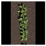
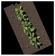
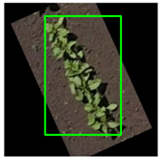
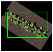
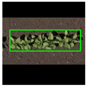
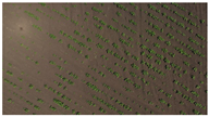
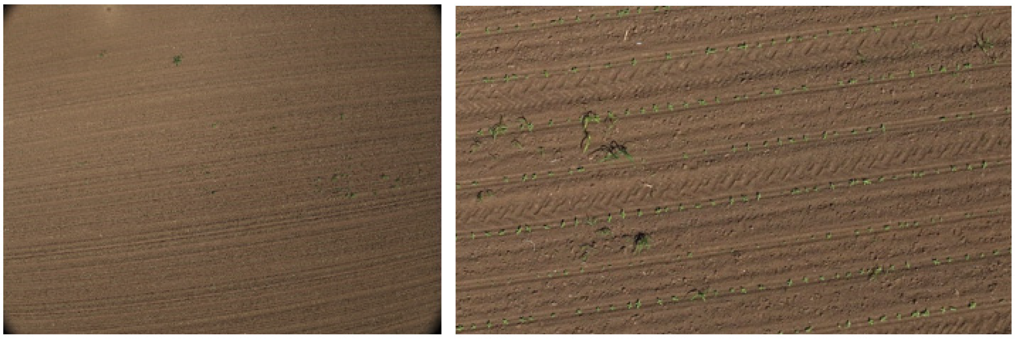
Our study focuses on cases where precision weed control is beneficial. We distinguish three main scenarios. The first case occurs when no crop is present, and only weeds are visible (
Figure 2a). The second case involves point-like crops arranged in rows, where the individual plants appear clearly separated (
Figure 2b). The third case is when the crops have grown to the point that they touch each other, forming continuous line segments (
Figure 2c). The example images presented in
Figure 2 were collected during UAV flights conducted on 13–14 May 2024. The image in
Figure 2a was taken on 13 May 2024, at GPS coordinates 46.101711, 18.742116. The images in
Figure 2b,c are part of a consecutive image series captured on 13 May 2024, at coordinates 46.072908, 18.709680
Figure 2b, and on 14 May 2024, at 47.772467, 19.621041
Figure 2c, respectively. A total of 208 images were used in the study, each containing 250–500 plants.
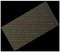
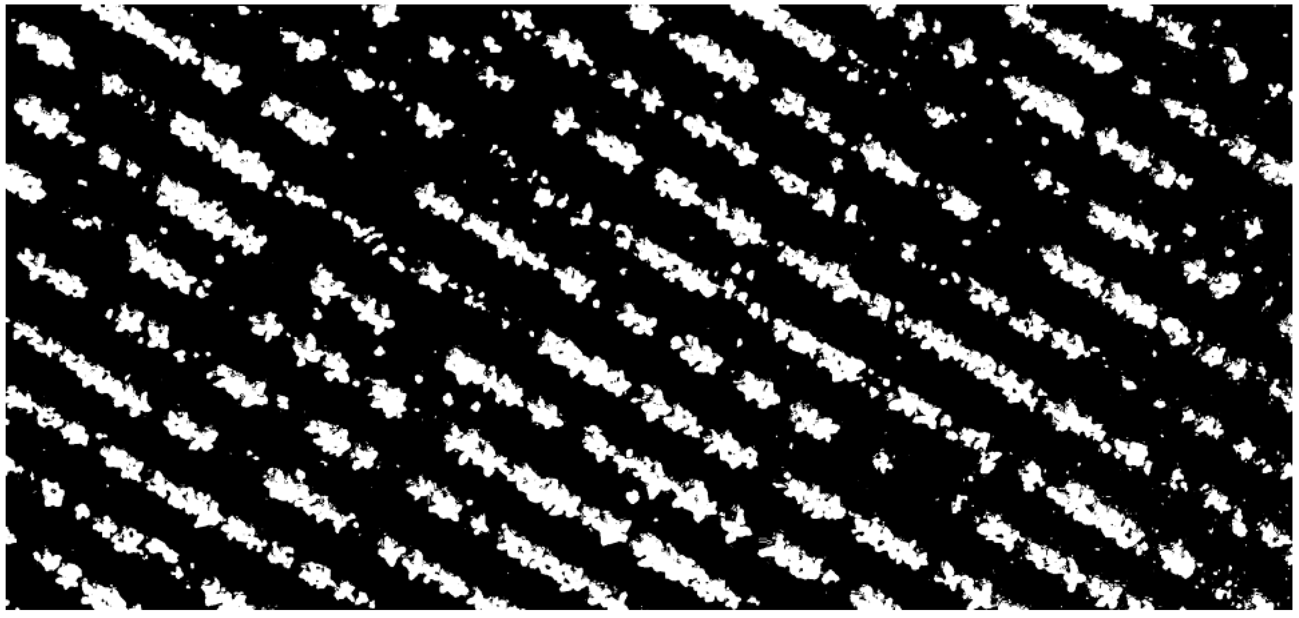
At the initial stage, similar computer vision procedures are applied. The RGB imagery is first converted into the HSV color space, in which the Hue channel carries the dominant color information. A thresholding technique is then employed to distinguish green-colored regions from the background. These green regions, which may represent either crops or weeds, are separated from the soil background based on their color characteristics.
The threshold image (
Figure 3) serves as the basis for the calculation process. The center point (x, y), height, and width of each object can be calculated and added to a list.
2.1. Only Weeds Present, No Crop Visible Case
In case (
Figure 2a), where no crop rows are visible, all detected plant instances are assumed to be weeds. This scenario represents the simplest case for generating weed density heatmaps or shapefiles. Further details regarding this approach can be found in our previous study [
4].
In this case, the coordinates and sizes of the weed instances are already available in a dataset. As each detection corresponds to a weed, spatial density maps can be generated directly. To accomplish this, information must be obtained from the farmer regarding the preferred operational grid size. The spatial grid can be defined in accordance with the technical specifications of the available weed control equipment, such as a row cultivator, a section-controlled spraying tractor, or a spraying drone. Each of these technologies imposes practical limitations on the grid resolution that can be applied with sufficient precision.
Once the grid size has been determined, two types of heatmaps can be generated. The first method involves counting the number of weed instances within each grid cell, without considering their spatial extent. In this case, each grid has a number of weeds inside. Alternatively, a coverage-based approach can be used, in which the cumulative area occupied by weed bounding boxes is calculated for each cell, resulting in a percentage-based coverage map that reflects weed pressure relative to the exposed soil surface. In this case, there is a number between 0 and 1 in each grid.
After the heatmaps have been computed, a threshold can be applied to convert the continuous values into a binary weed control map, indicating whether intervention is necessary in each grid cell. This binary map can be used to generate shapefiles suitable for precision weed management. Although multi-level thresholds and variable-rate weed control zones are technically feasible, only the binary classification approach was implemented in the present study.
2.2. Case Where Crop Rows Visible, Without Crop Overlap
In the second case (
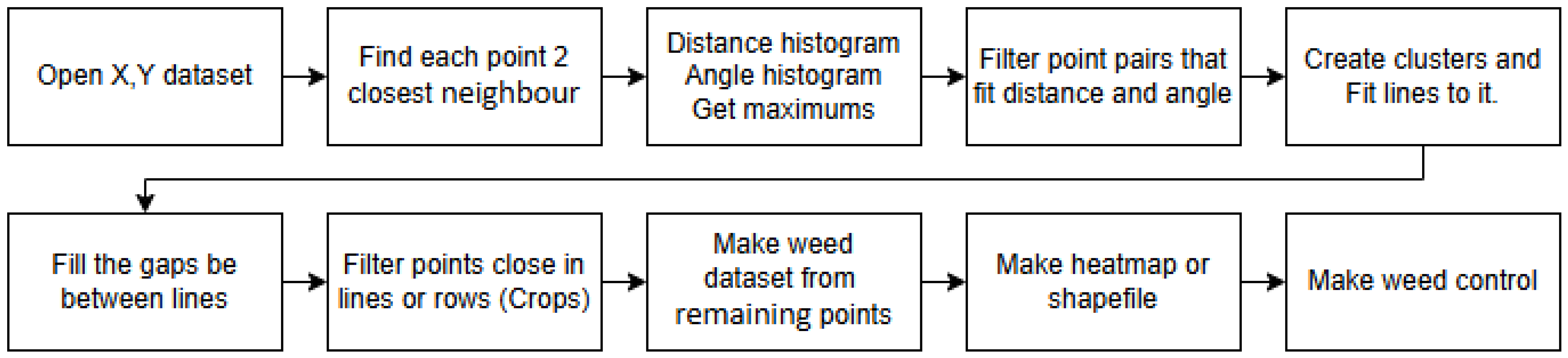
Figure 2b), the crops are clearly visible, and the rows are recognizable, but most plants are separated from one another. The second phase of the process, shown in
Figure 4, involves mathematical analysis.
In
Figure 5 (left), the image was captured by a UAV (Date: 13 May 2024 14:18:31, GPS Lat: 46.07290755, GPS Long: 18.70967997). The flight happened at a height of 21.7 m, resulting in a ground sampling distance (GSD) of 0.58 cm/pixel. The picture on the right shows the detailed structure of the crop rows with a few weeds interspersed among them. This detailed view emphasizes the spatial arrangement and contrast between the crop plants and weed distribution.
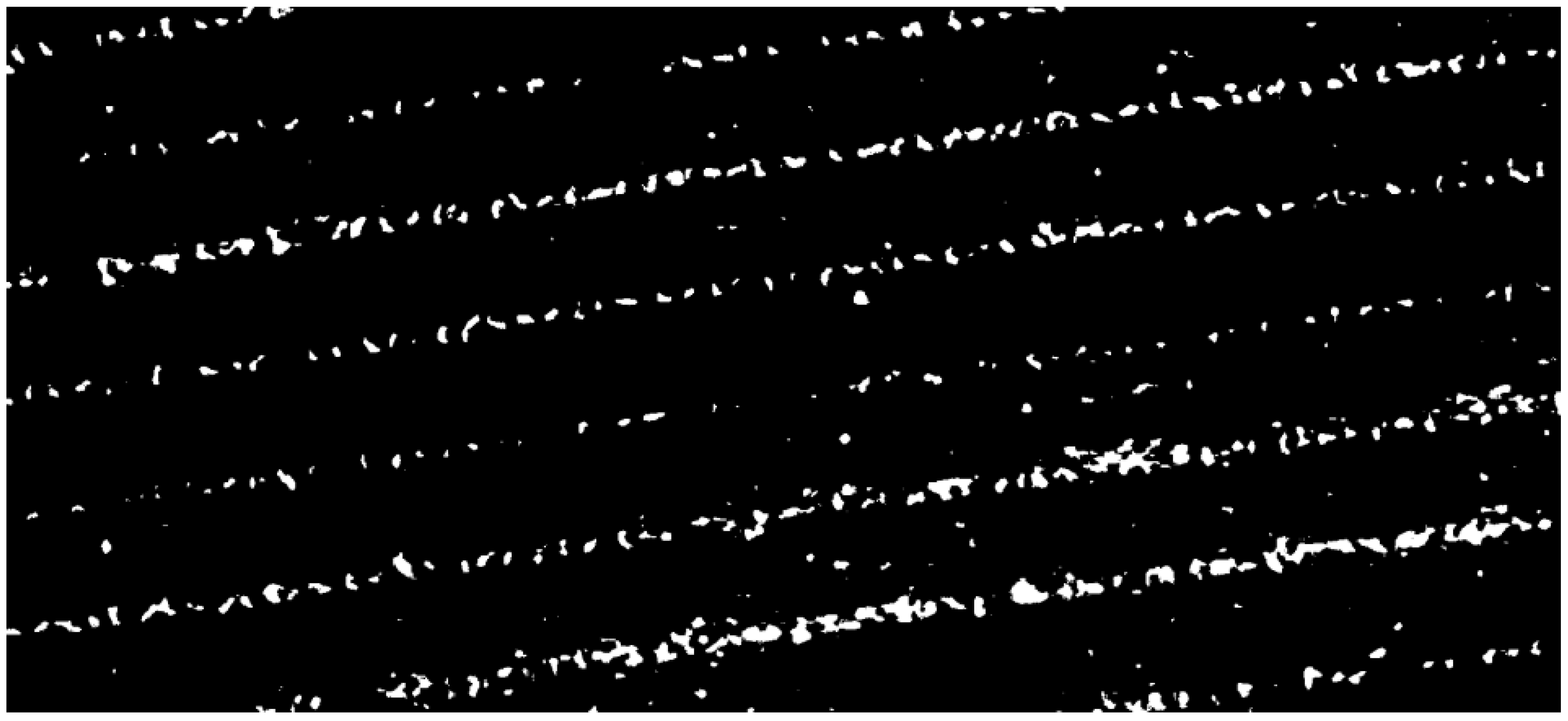
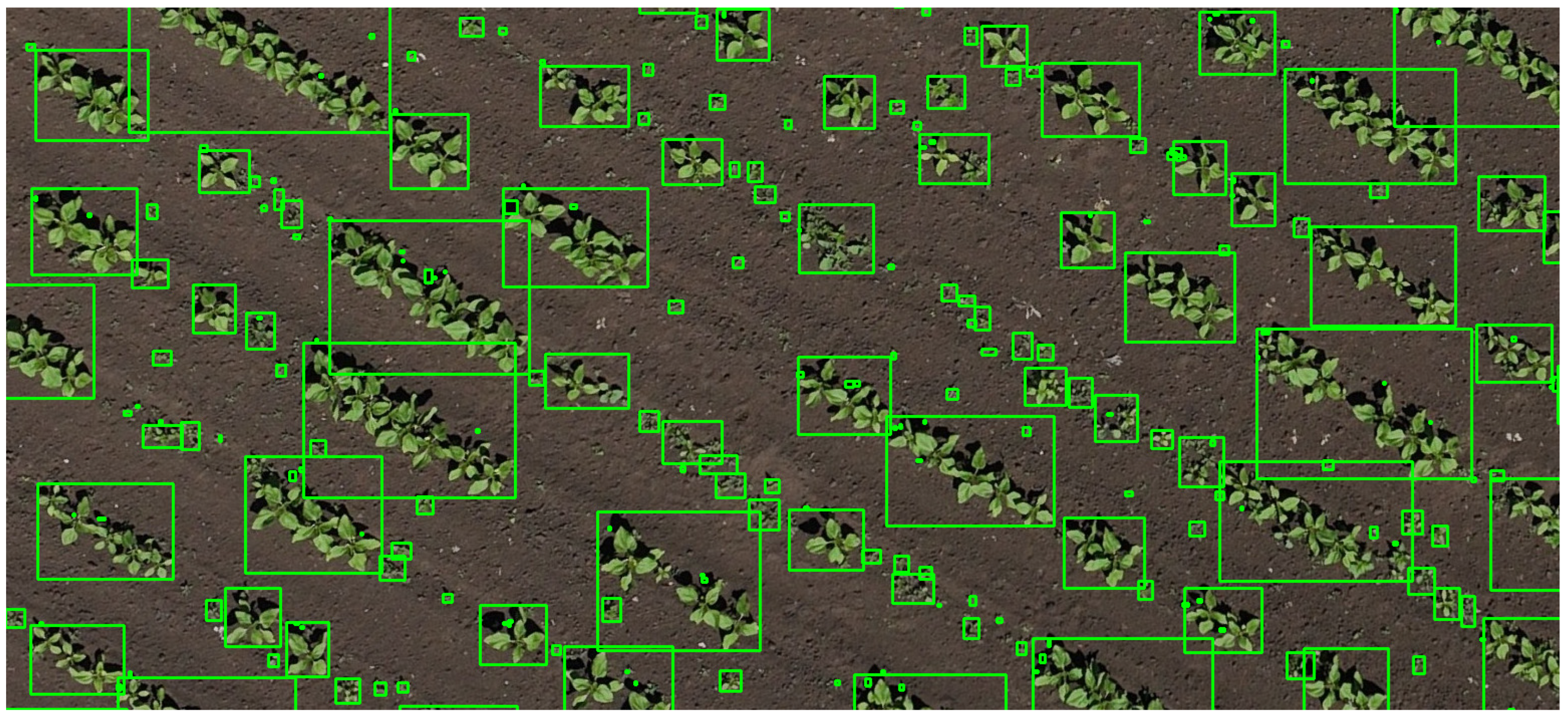
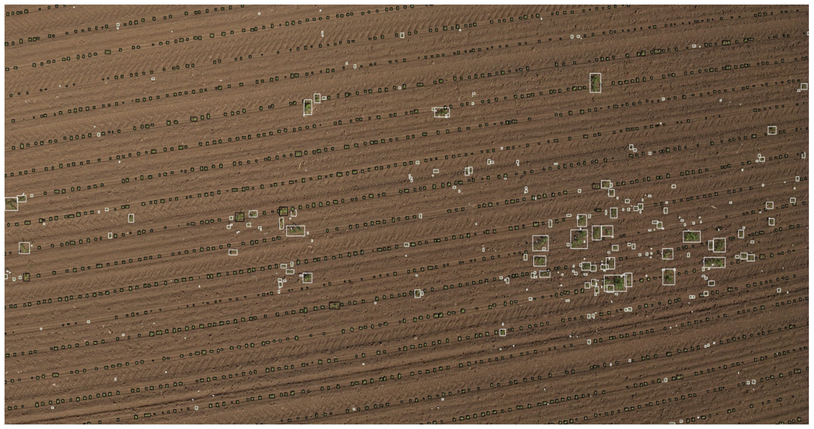
The same plant detection image processing workflow, as previously described, can be applied in this case. The resulting bounding boxes resemble those shown in
Figure 6, with each box representing an individual plant. These boxes of information were saved onto a csv file. However, no classification was performed at this stage to distinguish between crop plants and weeds. Due to the limited image resolution and observation distance, even domain experts are often unable to reliably differentiate between species based on visual characteristics alone. Consequently, it is necessary to incorporate structural information for accurate identification. It is assumed that the plants located within crop rows are crops, whereas those located outside the established row patterns are weeds.
The input was the CSV data file created earlier. For each point, the two nearest neighbors were identified, and the distance and angle relative to the horizontal between them were recorded. Using this data, two histograms were generated, from which the peaks were identified. Theoretically, weeds are randomly or sometimes group-located, so the minimum distances between them will show a range, and the angles will be evenly distributed in all directions. However, the spacing between crop plants is almost uniform, and their direction is similar. Thus, the two peaks theoretically indicate the direction of the rows and the distance between the plants.
Using these two parameters, point pairs that match the expected distance and direction were filtered out. Most of these points represent crop plants. Through proximity-based clustering, groups were formed, and lines or line segments were fitted to these groups. These lines represent the crop rows. The points near these lines were considered crop plants and were filtered out, leaving the remaining points as weeds located between the rows.
From these points, heatmap and management zones were generated in shapefile format. These outputs can then be used for variable-rate weed applications.
2.3. Crops Touching and Looking Like a Larger Object
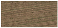
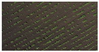
In the third scenario, referred to as case (
Figure 2c), crop plants may grow in such close proximity that they visually merge after the thresholding step, resulting in the formation of large, contiguous regions. As illustrated in
Figure 7, several crop instances may be grouped together and enclosed by a single, larger bounding box (
Figure 8). This outcome is problematic for clustering algorithms such as DBSCAN, which interpret these merged structures as single objects with no nearby neighbors, thereby compromising the row detection process.
To address this issue, an additional step is introduced to detect and handle such merged boxes. The first task involves identifying bounding boxes that are likely to represent clusters of multiple plants, rather than individual instances. These aggregated regions must then be segmented into smaller components to enable accurate spatial analysis and clustering in subsequent phases.
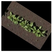
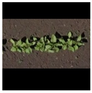
When individual crop instances are well separated, the bounding box dimensions tend to remain consistent, primarily influenced by the image acquisition angle and resolution. However, in cases where elongated crops have grown together along the crop row, significant variation in bounding box shapes may occur, particularly when the image is rotated. As demonstrated in
Table 1, the same image region—containing a continuous crop row—was analyzed after being rotated at four different angles. Bounding boxes were detected in each case, and the corresponding width and height values (in pixels) were recorded. To assess the geometric distortion, the width per height (W/H) ratio was computed for each box. The final rows of the table also include visualizations of the bounding boxes, highlighting the impact of rotation on object representation.
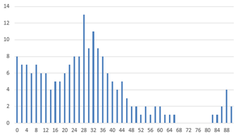
In the initial rotation case, where the crop rows are aligned vertically (top-down), and in the final case, where the rows appear horizontally, the detected bounding boxes remain relatively narrow. In contrast, the bounding boxes in the intermediate rotations become significantly wider. Based on this observation, a rotational analysis was performed by incrementally rotating the image and evaluating the W/H ratio of the detected bounding boxes.
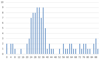
To this end, the image was rotated in 2-degree increments across a 0° to 90° range. For each rotation angle, bounding boxes were calculated, and their W/H ratios were calculated too. A histogram was constructed where each bin represents a rotation angle, and the corresponding value reflects the number of bounding boxes with a W/H ratio greater than 3. Boxes exceeding this threshold are considered to exhibit a strong horizontal alignment and are likely to represent segments of crop rows. Ratios below 3 are ambiguous, as they may correspond to elongated individual plants, clusters of weeds, or mixed crop-weed groups.
The histogram was then analyzed to identify the angle at which the maximum number of horizontally elongated boxes occurred. This angle was selected as the optimal rotation angle, aligning the crop rows horizontally in the image. Following this alignment, a second round of bounding box detection was performed.
In this step, each bounding box with a W/H ratio greater than 2 was subdivided into smaller, approximately square boxes. The number of subdivisions was determined by the ratio of W/H, with the original bounding box being split accordingly. For example, a box with a W/H ratio of 4.2 would be divided into four equally sized sub-boxes. As a result, the final dataset closely resembles the structure observed in case (
Figure 2b), where crops are well-separated. This standardized output allows for the application of the same row detection and line fitting algorithms used previously.
2.4. The Algorithms Visualization
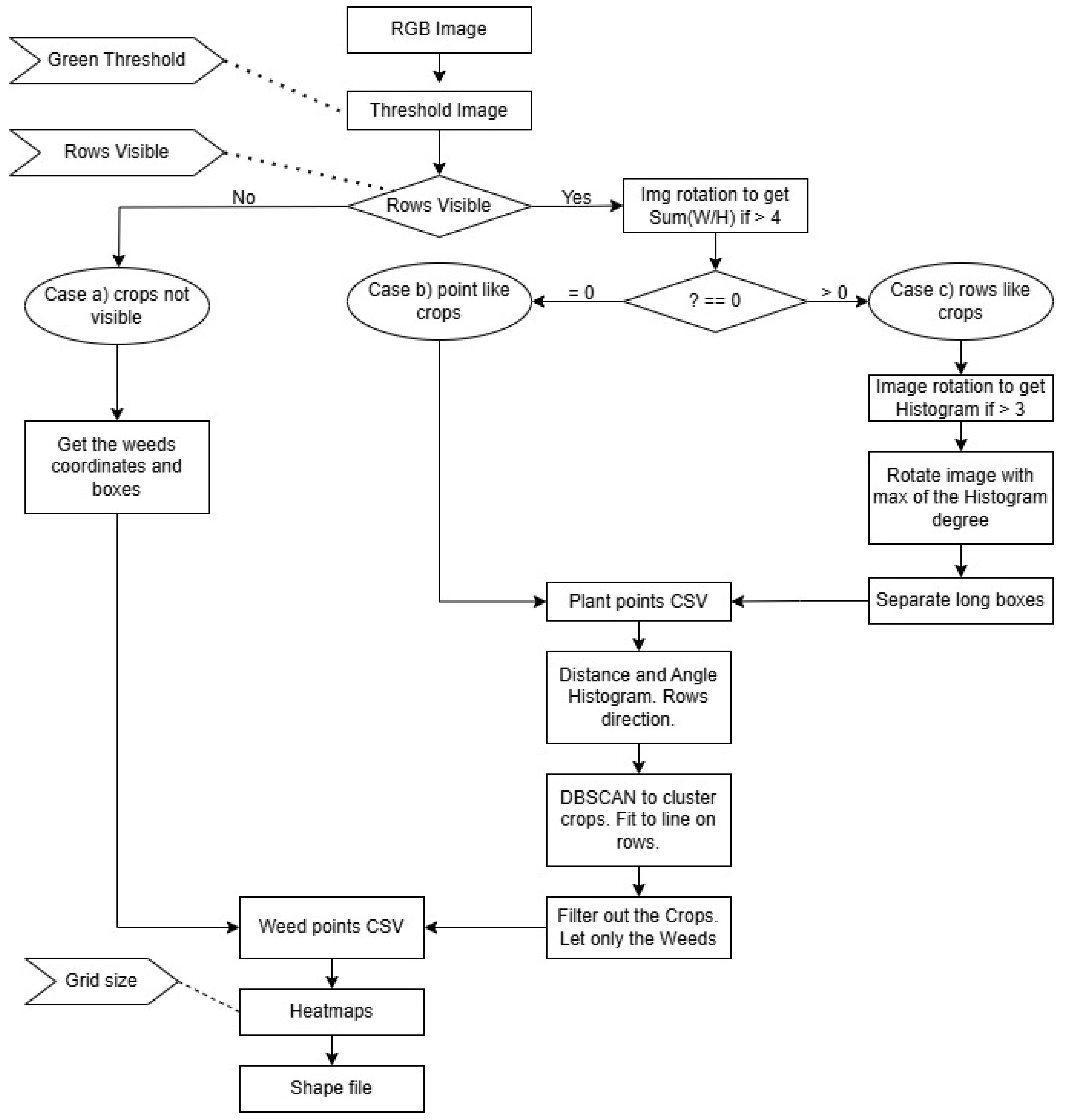
At this stage, the complete structure of the proposed algorithm can be outlined. The main processing steps are summarized in
Figure 9, which provides a comprehensive overview of the method. The process begins with three essential inputs provided by the farmer.
First, a “Green Threshold” value must be specified to achieve effective separation between vegetation and soil in the image. This threshold is used during the HSV-based segmentation step, where green plant regions are isolated.
Second, a binary input labeled “Rows Visible” is required to indicate whether crop rows are visible in the imagery. This decision determines which processing pathway is followed—either assuming all detected plants are weeds or employing row detection to distinguish between crop and weed instances.
Third, the “Grid Size” parameter must be defined. This value corresponds to the spatial resolution of the weed control equipment available to the farmer. Whether the treatment involves row cultivators, variable-rate spraying tractors, or spraying drones, each system operates optimally within a certain grid resolution. This input directly influences the resolution of the heatmaps and binary weed maps that are generated during the final stages of the algorithm.
The algorithm was evaluated on multiple images. When provided with accurate input parameters, it generally performed well. However, it was observed that the algorithm failed in specific cases where crop rows were faintly visible or heavily obscured by dense weed coverage. In such scenarios, both the distance histograms and the angle histogram produced misleading results. This occurred because the inter-weed distances were often shorter than the actual spacing between crop plants, leading to incorrect estimations of row spacing and orientation. Consequently, crop rows were not correctly identified, and the computed rotation angle was inaccurate.
Despite these discrepancies, the algorithm continued to process the data, resulting in bad heatmaps and shapefiles. To mitigate this issue, additional research was conducted to develop a validation mechanism that informs the farmer whether the output of the process is reliable.
2.5. Artificial Dataset for Border Case Determination
A critical consideration is determining the conditions under which the algorithm can be reliably applied. When weed pressure surpasses a certain threshold, the rows may become obscured, potentially compromising the functionality of an autonomous decision-making system.
To evaluate the algorithm’s robustness, its performance was tested using artificially generated crops and weed coordinates. The testing focused on two key parameters.
First, in practice, plants are not perfectly aligned in rows. Uniformly distributed noise was introduced in two dimensions to the ideal coordinates to simulate:
Alignment variability: Plants are rarely perfectly aligned in rows. This adjustment allowed plants to deviate to the left or right of a perfectly straight line, replicating the natural variability observed in fields.
Distance variability: Variability was also introduced in the spacing between plants. This noise simulated deviations in the ideal uniform distances, resulting in plants being sometimes closer together and sometimes further apart.
These controlled tests were essential for assessing the algorithm’s resilience to real-world inconsistencies and its capability to maintain accurate row and weed identification under varying conditions.
Random values were applied as follows: 0%, 1%, 2%, 3%, 4%, 5%, 6%, 7%, 8.5%, 10%, 15%, and 20% of the distance between plants.
The other parameter tested was the number of weeds. In the generated area, there were 678 crop plants. Weeds were added completely randomly. The number of weeds were: 0, 200, 400, 600, 800, 1000, 1200, 1500, 2000, and 3000.
120 datasets were generated and performed calculations on each one. For each dataset row directions were calculated, the average distance between plants, the total number of points, the number of points classified as being on a row or line, and the number of clusters, which corresponds to the number of line segments detected (with the original number of rows being 18). After performing the clustering, a calculated class was assigned to each point. Additionally, the precision, recall, F1 score, and accuracy were computed. F1 score is a metric combining precision and recall using a harmonic mean, where “1” indicates that precision and recall are equally weighted, i.e., β = 1 in the general Fβ formula.
In the Results section, several tables were created. Each table contains 120 data cells, with each cell representing a different scenario from the 120 artificial datasets.
The headers of the tables show the percentage values of crop disturbance noise that was artificially generated. A value of 0% means the crop rows are perfectly parallel, with equal spacing between the plants. The last column, marked 20%, represents a scenario where the crops in the rows appear quite randomly. Some crops are still aligned within rows, but the spacing between them varies significantly.
The rows of the tables indicate how many weeds were added to the area, which originally contained 678 crops arranged in 18 rows.
The first row (value 0) represents datasets that contain only crops and no weeds.
The last row (value 3000) represents a highly weedy scenario, where 3000 random weeds are added to the same area that still contains only 678 crops.
3. Results
3.1. Calculation Rows from Points
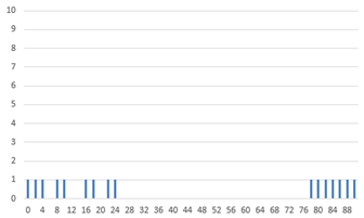
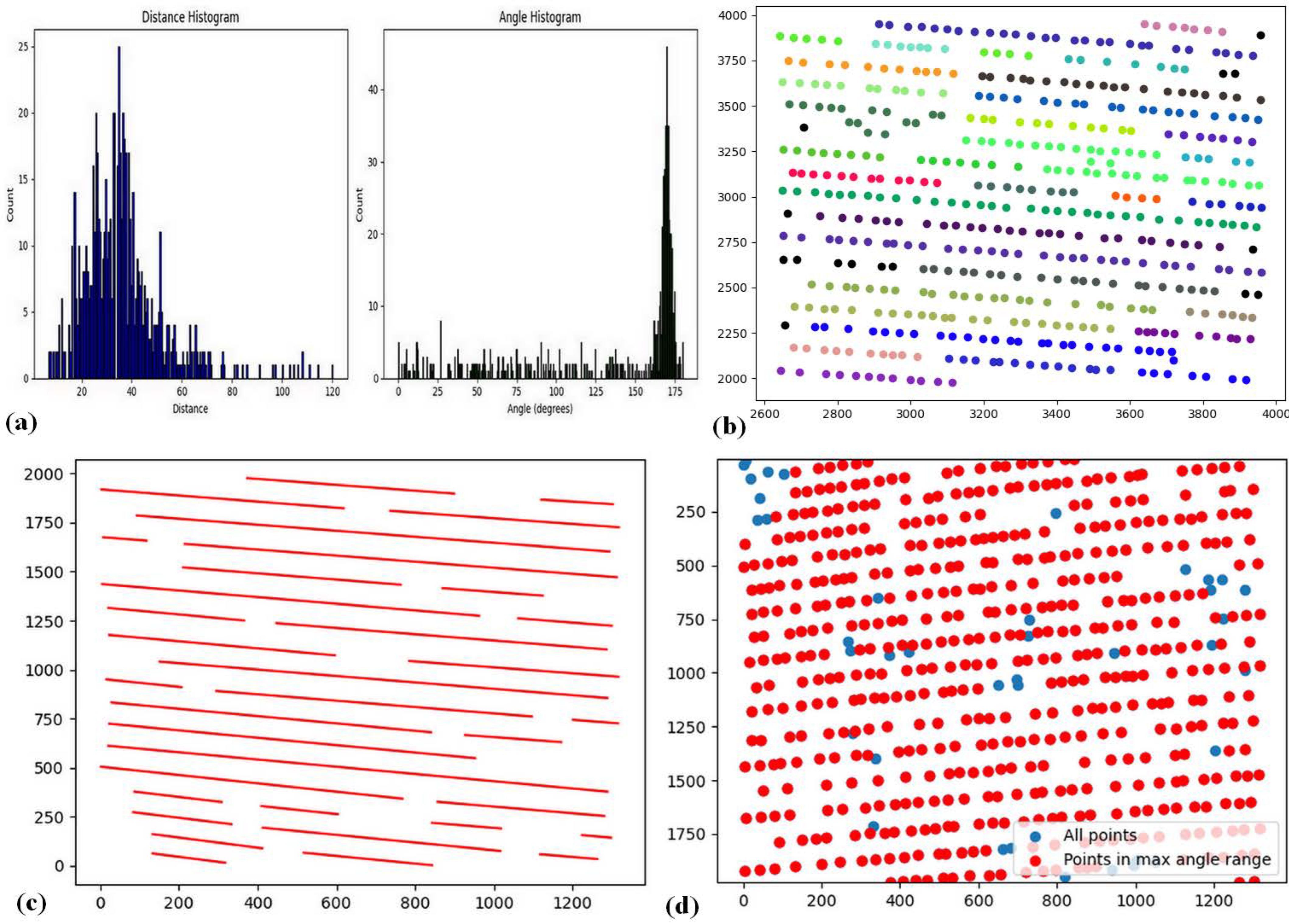
The analysis begins with the plant point dataset in CSV format. Initially, all plant coordinates were extracted, and for each point, the nearest neighbor was identified. The Euclidean distance and the angle relative to the horizontal axis were then calculated. Two histograms were generated based on these parameters, as illustrated in
Figure 10a.
Crop plants typically maintain consistent spacing, resulting in a prominent peak in the distance histogram. In contrast, weed distances are more variable and occur with less frequency. Consequently, the peak of the distance histogram is assumed to represent the average crop spacing. A similar approach is applied to the angle histogram, where the maximum value indicates the predominant crop row orientation. Weeds, on the other hand, tend to deviate from this dominant direction.
Using these two parameters—interplant distance and row angle—thresholds were applied to identify likely crop points. A DBSCAN clustering algorithm was then executed on the filtered crop points, with the resulting clusters shown in
Figure 10b. Linear regression was subsequently applied to each cluster to fit line segments representing the crop rows (
Figure 10c). After interpolating between the detected row segments, the classification of all plant points was refined: points located on or near the lines were classified as crops, while those situated between rows were classified as weeds (
Figure 10d).
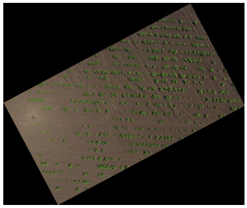
Figure 11 illustrates the original image with an overlay: black markings indicate the locations of crop plants, while white markings represent the positions of weeds. The visualization reveals a clear pattern in the spatial distribution of weeds, which tend to cluster in certain areas. Additionally, some zones are entirely devoid of weeds, highlighting the variation in weed density across the field.
The results indicate that crop rows can be successfully detected. Although there were occasional misclassifications (some crops being detected as weeds or weeds eliminated as crops), these errors were rare, and the overall weed detection accuracy was good. Most weeds were found between rows, and the resulting heatmap accurately reflects weed pressure.
3.2. Crops Rotation Results
The algorithm described above operates on datasets composed of individual plant coordinates. However, ideal conditions are not consistently present; in many cases, the crop plants exhibit significant overlap. Under such circumstances, the bounding boxes often enclose multiple plants rather than a single one. Consequently, prior to applying the coordinate-based method, it is essential to divide these larger bounding boxes into smaller segments. This segmentation is achieved using a rotation-based algorithm supported by rotation histograms.
For each bounding box, the W/H ratio was calculated. A rotation histogram was then constructed by rotating the image in small angular increments (e.g., 2°) from 0° to 90° and recording the frequency of bounding boxes where the width was at least four times greater than the height. This criterion was used to identify elongated boxes that likely contain multiple plants aligned along crop rows.
The values from the rotation histogram were aggregated and referred to as the parameter R, as shown in
Table 2. A high R value suggests the presence of bounding boxes that may contain four or more plants, indicating the likelihood of crop row segments. If no such bounding boxes were detected across all rotation angles (R = 0), the image was considered to contain isolated, point-like plants. In such cases, the scenario matches
Figure 2b, and the crop row detection can proceed using the point-based algorithm described previously. Conversely, if R > 0, it suggests the presence of row structures and indicates that a different approach was required to detect and process these aligned plant groupings.
If R > 0, the image was incrementally rotated from 0° to 90°. For each rotation, the histogram of the bounding box aspect ratios (where W/H > 3) was generated—referred to as the rotation-rate–aspect ratio histogram. The rotation angle corresponding to the maximum histogram value was selected as the estimated row direction. Based on this angle, the image was rotated accordingly to align with the crop rows horizontally.
Following this alignment, the elongated bounding boxes representing overlapping plant clusters can be subdivided into smaller, nearly square segments. This process allows for reconstructing a point-like plant dataset, which can then be processed using the previously described crop row detection algorithm based on plant coordinates.
As illustrated in
Table 2, six example cases are presented. The first three images contain well-separated plants, while the last three include overlapping rows with three different row orientations. In each case, the algorithm successfully identifies the dominant orientation and rotates the image to achieve horizontal alignment, as shown in the final column.
3.3. Heatmap Result
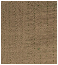
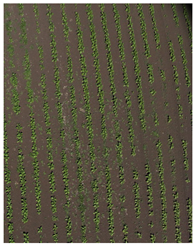
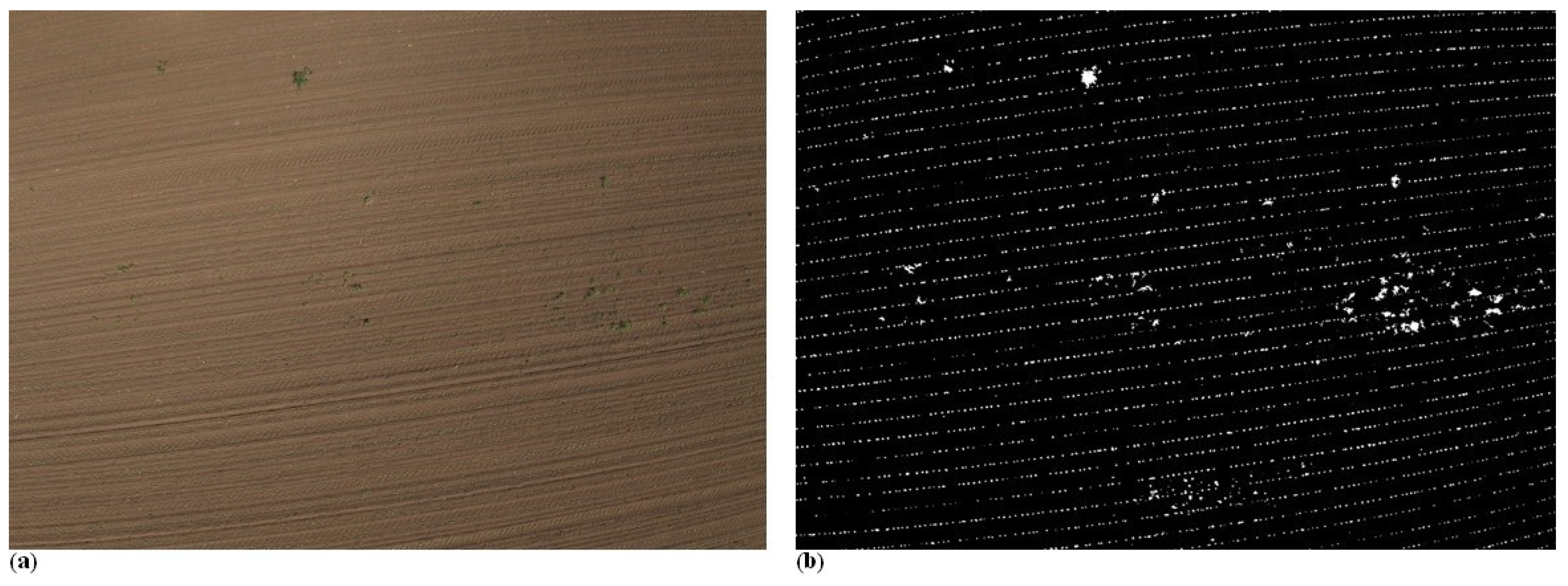
A weed pressure map was generated for a sunflower field, where crop rows were clearly visible, and weeds were present between the rows as point-like features. The original UAV image is shown in
Figure 12a, where both the sunflower rows and the inter-row weeds can be distinguished.
Next to it,
Figure 12b presents a binary image highlighting the green vegetation areas. After applying the proposed image processing algorithm, the crop rows were filtered out, and the remaining vegetation was classified as weeds. Based on these detected weeds, heatmaps were generated to visualize the spatial distribution and intensity of weed infestation.
Figure 13a presents the remaining vegetation after the crop rows were filtered out by the algorithm. These residual objects were considered weeds.
To generate weed pressure heatmaps, the algorithm requires a predefined grid cell size. This parameter depends on the technical specifications of the weed control equipment, particularly the spatial resolution of its application sections. One possible grid configuration is shown in the image on the right (
Figure 13b). This heatmap version visualizes the number of weed objects detected within each cell. This represents one approach to quantifying weed infestation.
The second approach (
Figure 14a) involves calculating the weed coverage within each cell, rather than simply counting the number of detected weed objects. In this case, it is possible that one cell contains a large number of small weeds, while another cell includes only one or two significantly larger weed patches. As a result, cells with extensive individual weeds are assigned higher values, reflecting the actual area covered by the vegetation.
For any type of heatmap, a threshold value can be defined to distinguish between areas that require weed control and those that do not. When that threshold was applied, the heatmap was transformed into a binary treatment map. Values below the threshold were considered insignificant and were excluded from weed management, while values above the threshold indicate zones where intervention is necessary. The selection of this threshold should ideally be determined by an expert, taking into account the specific agronomic and operational conditions. An example of such a binary output is shown in
Figure 14b, where weed control should be performed in the white-marked areas.
3.4. Artificial Dataset Results
The artificial dataset results are summarized in tables, presenting the performance of the algorithm across varying conditions. The table consists of 12 columns (rows noise) corresponding to the percentage of positional noise applied to the plant coordinates—the base is the crops distance—and 10 rows representing the number of weeds added to the area, resulting in a total of 120 data points.
In the generated sample, the plant spacing was predetermined at 22 pixels, while the spacing between rows was set at 67 pixels. Additionally, the rows were arranged at a 20-degree angle relative to the horizontal axis. Values in the table that are close to 22 pixels indicate that the algorithm successfully determined the plant spacing. These results reflect the algorithm’s capability to accurately extract crop plant arrangements under certain conditions.
However, in cases where the calculated spacing deviated significantly from 22 pixels, the algorithm failed to reliably determine the plant spacing. Such deviations were primarily associated with higher levels of positional noise or greater weed density, conditions that interfere with the algorithm’s ability to distinguish crop rows from background clutter. These findings highlight the impact of noise and weed pressure on the system’s performance and the conditions under which it can be effectively applied.
In
Table 3, cases where the plant spacing was accurately determined are highlighted, providing critical insights into the algorithm’s performance. The findings reveal that at very high weed densities, the proximity of weeds to one another becomes smaller than the spacing between crop plants. Under such conditions, the algorithm cannot reliably determine crop spacing, and the clustering process fails to detect crop rows. The system’s limit was identified at approximately two times the number of crops, or around 1200–1500 weeds relative to 678 crop plants. At this threshold, the algorithm was still able to determine crop spacing with reasonable accuracy, but performance degraded beyond this point.
Positional noise in plant coordinates further impacted the system’s ability to determine the spacing between crops, especially at higher noise levels. However, in real-world fields using real-time kinematics (RTK) systems, indicating that this factor is unlikely to limit the algorithm’s performance in practical applications.
The calculated row direction angle shows a pattern similar to that observed for plant spacing. At higher weed densities, determining the direction of crop rows became infeasible due to the overwhelming presence of weeds, which obscured the alignment of the crops. This underscores the sensitivity of the system to weed density and its importance in ensuring accurate detection of crop rows in autonomous agricultural applications.
Table 4 outlines the number of row segments or clusters identified by the algorithm compared to the actual 18 rows present in the sample. The interspersed weeds between the rows disrupted the detection of continuous rows, fragmenting them into multiple smaller segments. With 678 crop points distributed evenly across the 18 rows, each row initially contained an average of 37 plants. However, in extreme cases, the algorithm detected up to 80 clusters, which corresponds to an average of 4–5 segments per row. Each cluster contained approximately 8–10 crop plants, which proved sufficient for stable row identification under most conditions.
Instances where the algorithm detected fewer clusters than the actual number of rows are highlighted in red. These cases indicate unreliable performance, as the system incorrectly grouped weeds and crops into a single cluster, rendering the output unsuitable for accurate row detection. This limitation underscores the impact of excessive weed density on the system’s effectiveness.
Table 5 provides a detailed analysis of classification performance metrics—precision, recall, F1-score, and accuracy—for specific scenarios with 1% and 4% crop disturbance and varying weed densities of 200, 600, and 1200. These metrics illustrate the algorithm’s ability to correctly classify crops and weeds under different conditions. Performance generally declined as weed density increased, especially when combined with higher levels of crop positional disturbance. These results emphasize the need to manage weed density and maintain precise crop spacing to optimize system reliability.
The metrics indicate that variations in the unevenness of crop plants have minimal impact on the system’s performance, making this parameter less critical. However, the algorithm is highly sensitive to weed density, with performance varying significantly across different levels of weed pressure.
Low weed pressure: When weeds constitute approximately 30% of the total crop count, the algorithm performs with high accuracy, reliably identifying both weeds and crop plants. This demonstrates its capability to support precision agriculture under low-weed conditions effectively.
Moderate weed pressure: When weed density is roughly equal to the crop count, the system achieves an F1 score and accuracy of around 85%. This indicates that in 85% of cases, the algorithm correctly distinguishes between weeds and crops based solely on positional data. This performance level is sufficient for designing targeted weed control strategies.
High weed pressure: At weed densities approximately double the crop count, the algorithm’s accuracy drops to about 76%. While still significant, the reduced precision under such conditions suggests that total weed control methods may be more appropriate than targeted interventions at this level of infestation.
These findings underscore the importance of adapting weed management strategies based on weed density levels. The system demonstrates robust performance under moderate conditions but faces challenges with high weed pressure.
Table 6 presents the IRCR, defined as the ratio of all detected points to those classified as in-row points. For instance, if the algorithm detects 1000 plants in total and classifies 800 as “crops” based on neighbor angles and distances, the IRCR equals 1.25.
This ratio offers a practical decision-making tool for precision agriculture. By analyzing intermediate values calculated by the algorithm, such as the IRCR, it becomes possible to assess the reliability of row and weed detection without requiring prior knowledge of field parameters (e.g., specific crop distances and angles). This capability enhances the algorithm’s utility in diverse agricultural settings, providing a flexible framework for real-time decision-making.
The described methodology for applying the IRCR offers a practical framework for assessing the reliability of crop and weed detection, ultimately guiding weed management decisions in precision agriculture.
Parameter calculation: The algorithm determines the total number of plants in a defined area, separately identifying how many of these plants are located in positions consistent with crop plants based on expected spacing and alignment.
IRCR analysis: The IRCR is calculated by dividing the total detected plants by the number classified as in-row crop plants. This ratio serves as a quantitative measure of the algorithm’s ability to distinguish between crops and weeds.
Threshold for reliability: A critical threshold for the IRCR was established at 4.5. Ratios below this threshold indicate reliable performance, demonstrating that the algorithm has accurately detected crop rows and distinguished weeds, even in real-world conditions where specific crop spacing and row orientations are unknown. Conversely, an IRCR exceeding 4.5 suggests that the system has struggled to reliably identify crop rows, likely due to high weed pressure. In such cases, a shift from precision weed control to total weed control is recommended to ensure effective field management.
In summary, this methodology provides an operational decision-making tool that uses the IRCR to assess field conditions and guide weed control strategies. A ratio below 4.5 supports the use of precision weed management, while higher ratios signal the need for more aggressive approaches due to challenging field conditions.
The average valid IRCR values highlighted in green in
Table 6, along with the correlation analysis, further validate this approach. The observed correlation between the calculated IRCR and actual weed-to-crop ratios is approximately 99%, confirming the strong relationship between the IRCR and weed pressure
Table 7. This high correlation underscores the robustness of the IRCR as a reliable indicator of the field’s condition and the system’s detection accuracy, making it a practical and data-driven guide for optimizing agricultural practices.
4. Discussion and Conclusions
This study demonstrates that weed pressure heatmaps and shapefiles can be effectively generated from UAV images without requiring significant computational resources or extensive training datasets. The method is highly adaptable, functioning independently of crop type, weed species, or developmental stage, as long as crop rows are visible and recognizable. Importantly, the method does not demand high-resolution, detail-rich imagery; UAVs can capture usable images from altitudes between 20 and 30 m. Moreover, it accommodates scenarios where crop plants are spaced apart and do not form a continuous canopy within the rows.
Most row detection algorithms need visible strong rows. Moreover, they usually work on land-based images. Our approach was to make aerial imaginary and make usable weed control maps and weed pressure maps.
Analyzing the images, there were some well-defined cases: for example, the total plant-free areas had no need for weed control at all, while the totally weedy green images needed total weed control.
The other cases were more interesting and more relevant for precision weed control. Three main cases were found here.
First case: There were weeds in the area, but no crops yet. It was a straightforward solution. We took the weed coordinates and created weed pressure maps.
Second case: There were weeds and crops, but the crops still stood alone. They had small sizes and had not reached each other yet. Here, we used mathematical and statistical methods to classify or separate the weeds from the crops. After classification, we used only the weeds’ coordinates, and, similar to the first case, we could create the weed pressure maps.
Third case: There were weeds and crops, but the crops were bigger and started to overlap. Here, computer vision was applied to rotate the images; still, the rows had a vertical position. On this rotated image, it was possible to split the crops into smaller segments; as a result, we obtained similar coordinates and box dataset to the second case. So, after the second case, the algorithm steps were able to generate the weed pressure maps for us.
The algorithm performed well in most cases; however, when the number of weeds significantly exceeded the number of crop plants, it was unable to detect the crop rows reliably. To determine the operational limits of our algorithm, we generated 120 artificial datasets. Based on the analysis of these datasets, we developed a self-diagnostic parameter capable of identifying areas that are too heavily infested with weeds for accurate row detection, indicating the need for total weed control instead.
The study establishes that the algorithm is robust enough to function in areas where the weed density is up to twice the crop density, allowing detection of crop lines even in heavily infested fields. Beyond this threshold, however, the crop lines become obscured when using coordinate-based analysis alone, necessitating a shift from precision weed management to total weed control.
A key outcome of this work is the development of the IRCR as a diagnostic parameter. If the IRCR exceeds 4.5, the field conditions are deemed too weedy for accurate row detection, and parameters such as row direction are no longer valid. Conversely, when the IRCR is below 4.5, the calculated parameters, including row positions, remain reliable. This parameter correlates strongly (approximately 99%) with the actual weed-to-crop ratio, highlighting its potential as an indicator for adaptive weed control strategies, such as varying the intensity of weeding interventions based on localized conditions.
This flexible and efficient approach provides a valuable tool for precision agriculture, enabling targeted weed management strategies across diverse crop systems and field conditions.
Our approach differs from the most existing methods, which generally rely on land-based or low-altitude imagery where crop rows are highly visible. These conventional techniques often depend on high-resolution data or deep learning models trained on extensive annotated datasets. In contrast, our coordinate- and statistics-based method enables robust weed mapping even when crops are spaced apart and have not yet formed continuous canopy within rows.
The algorithm performed reliably across these scenarios, achieving precision and recall above 95% when weed density was up to 30% of crop count, and F1 scores of around 85% even when weed and crop densities were equal. However, performance declined when weed density exceeded crop density by a factor of two or more, with precision and recall falling below 76%. In such cases, crop rows became obscured, and the method recommended shifting from precision control to total weed control.
In comparison with other aerial-based weed mapping studies, our method offers clear operational advantages. For instance, Huang et al. conducted UAV flights at just 6 m altitude, requiring about four times longer flight durations and generating 16 times more images for processing and storage. While their imagery supported CNN-based pixel-level classification, the approach was less scalable for large areas [
14]. Similarly, Castellano et al. used UAV imagery captured at 10 m altitude, with individual crops spanning 15–20 pixels and weeds 5–10 pixels. Their method required multispectral cameras and neural networks, resulting in 2–3 times more flights and 4–5 times more images, along with higher equipment costs [
15]. Marinis et al. rotated UAV images to align crop rows, like us, and faced similar limitations under high weed density, discarding data when row detection was unreliable. They applied Hough transformation for row detection and required annotated training data for their neural network classifier, achieving an F1 score of 75.3 [
16].
In summary, our lightweight and unsupervised coordinate-based method enhances the practicality and scalability of UAV-based weed mapping, enabling targeted management strategies across diverse agricultural settings with minimal resource requirements.


