Article

Maize Seed Variety Classification Based on Hyperspectral Imaging and a CNN-LSTM Learning Framework

1
School of Technology, Beijing Forestry University, Beijing 100083, China
2
School of Agricultural Engineering, Jiangsu University, Zhenjiang 212013, China
3
Key Laboratory for Theory and Technology of Intelligent Agricultural Machinery and Equipment, Jiangsu University, Zhenjiang 212013, China
*
Author to whom correspondence should be addressed.
Agronomy 2025, 15(7), 1585; https://doi.org/10.3390/agronomy15071585
Submission received: 22 May 2025 / Revised: 21 June 2025 / Accepted: 26 June 2025 / Published: 29 June 2025
(This article belongs to the Collection AI, Sensors and Robotics for Smart Agriculture)

Abstract

Maize seed variety classification has become essential in agriculture, driven by advancements in non-destructive sensing and machine learning techniques. This study introduced an efficient method for maize variety identification by combining hyperspectral imaging with a framework that integrates Convolutional Neural Networks (CNNs) and Long Short-Term Memory (LSTM) networks. Spectral data were acquired by hyperspectral imaging technology from five maize varieties and processed using Savitzky–Golay (SG) smoothing, along with standard normal variate (SNV) preprocessing. To enhance feature selection, the competitive adaptive reweighted sampling (CARS) algorithm was applied to reduce redundant information, identifying 100 key wavelengths from an initial set of 774. This method successfully minimized data dimensionality, reduced variable collinearity, and boosted the model’s stability and computational efficiency. A CNN-LSTM model, built on the selected wavelengths, achieved an accuracy of 95.27% in maize variety classification, outperforming traditional chemometric models like partial least squares discriminant analysis, support vector machines, and extreme learning machines. These results showed that the CNN-LSTM model excelled in extracting complex spectral features and offering strong generalization and classification capabilities. Therefore, the model proposed in this study served as an effective tool for maize variety identification.

1. Introduction

Maize is a critical food crop in China, serving not only as a staple food but also as a key source of animal feed and industrial raw materials. The production of maize is vital for ensuring China’s food security [1]. With continuous innovations and improvements in biological breeding technologies, such as molecular marker-assisted breeding, the number of maize varieties has been steadily increasing. However, challenges such as substandard varieties and variety infringement are widespread, posing new difficulties in accurately identifying and ensuring the purity of maize seeds.
Accurate identification of maize varieties is crucial for maintaining seed quality, improving maize yields, standardizing the seed market, and fostering the healthy development of the maize industry [2]. Visually distinguishing between maize varieties can be challenging because of their similar appearance. Traditional methods for identifying varietal authenticity, such as seedling morphology, isozyme and seed storage protein identification, and molecular marker techniques like simple sequence repeat (SSR) technology, come with significant drawbacks [3]. These methods are often labor intensive, time consuming, environmentally impactful, and costly.
Hyperspectral imaging technology, which integrates both spectral and image analyses, has emerged as a promising solution [4,5]. It provides richer spatial and spectral information than traditional near-infrared spectral analysis, making it an ideal tool for seed quality detection [6]. This technology has been widely used in assessing seed composition and detecting characteristics such as cracks, molds, and other defects [7,8,9,10]. In seed variety identification, Xia et al. [11] used hyperspectral images of seeds from 17 varieties in the 400–1000 nm range and multivariate linear discriminant analysis to develop a maize variety classification model. A feature wavelength screening algorithm to extract key spectral information from hyperspectral data was used, creating a model based on feature wavelengths to distinguish sweet corn varieties [12]. Similarly, Jiang et al. [13] used a BP-Adaboost model to identify 10 wheat seed varieties, while Wang et al. [14] applied an extreme learning machine algorithm combined with feature wavelength screening to effectively identify eight maize seed varieties.
Whilst the majority of studies utilized conventional machine learning algorithms for data processing, recent advancements in deep learning—particularly the Convolutional Neural Network (CNN)—has considerably enhanced the extraction of features, classification, and object detection [15,16]. Despite the advances achieved, the application of deep learning in the processing of one-dimensional spectral signals has remained constrained. The integration of near-infrared hyperspectral imaging with a CNN was employed for the classification of barley seed diversity [17], which demonstrated that the CNN model exhibited a marked superiority over conventional approaches, attaining an accuracy over 98%. It is noteworthy that the classification accuracy for 29 hulled barley varieties and 6 naked barley varieties reached 98.28% and 98.36%, respectively, demonstrating the superior performance of CNNs in comparison to conventional machine learning methods.
Que et al. [18] employed three distinct spectral wavelength interval selection methods to extract feature wavelengths. These were then integrated with group convolution to construct a CNN. This approach resulted in a substantial enhancement in both the classification accuracy and the inference speed for the classification of wheat. The Long Short-Term Memory (LSTM) network, a variant of Recurrent Neural Networks (RNNs), has been shown to capture higher-order feature information in sequential data and address the long-term dependency problem inherent in RNNs [19]. Consequently, LSTM demonstrates particular proficiency in the representation of models and the accuracy of prediction in the context of sequential data. Zhou et al. [20] employed an LSTM model to extract and analyze pixel-level spectral features and spatial characteristics for the classification of hyperspectral images across three widely utilized hyperspectral datasets. The following institutions have been represented: Indian Pines, Pavia University, and Kennedy Space Center. The efficacy of the proposed method was demonstrated by a significant enhancement in classification accuracy, with improvements of 2.69%, 1.53%, and 1.08%, respectively, in comparison to contemporary state-of-the-art techniques. The findings of these studies emphasized the superior capabilities of both the CNN and LSTM in spectral analysis [21]. CNNs have been shown to be effective in the extraction of spectral features. However, LSTM networks have been demonstrated to excel at capturing interdependencies between these features, thereby enabling the selection of the most relevant patterns for the data [22]. However, the integration of a CNN and LSTM for seed variety classification using hyperspectral imaging remains an under-explored field.
The objective of this study was to evaluate the synergy of a CNN and LSTM for the efficient and rapid identification of maize varieties based on hyperspectral imaging. Moreover, a thoroughgoing comparison is conducted with conventional machine learning algorithms, including partial least squares discriminant analysis (PLS-DA), a support vector machine (SVM), and an extreme learning machine (ELM), with regard to the model’s capacity for generalization and its resilience.

2. Materials and Methods

2.1. Sample Material Preparation

Five maize seed varieties—Jingke 968 (JK968), Xianyu 335 (XY335), Zhengdan 958 (ZD958), Jundan 20 (JD20), and Denghai 605 (DH605)—were sourced from Henan Kunyu Seed Company. (Zhengzhou, Henan Province, China). A total of 810 fully matured, intact seeds from each variety were meticulously selected to ensure uniformity and high quality for analysis (Table 1). The seeds were randomly divided into two groups: about 70% were allocated to the training set, and the remaining samples were regarded as prediction set. The objective of this division was to maintain a balance between training and prediction, which were used to model development and model evaluation, respectively.

2.2. Hyperspectral Imaging Acquisition

A line-scan hyperspectral imaging system was employed to capture hyperspectral reflectance images of maize seeds. The system comprised multiple essential components, including an imaging spectrograph (ImSpector V10E, Spectral Imaging Ltd., Oulu, Finland) with a spectral range of 319–1099 nm and a nominal spectral resolution of 2.8 nm, an EMCCD camera (Andor Luca EMCCD DL-604M, Andor Technology plc., Oxford, UK)with a resolution of 1004 × 1000 pixels, a lens (OLE23-f/2.4, Spectral Imaging Ltd., Oulu, Finland), two halogen lamps positioned at a 45° angle for optimal illumination, and a displacement stage for precise sample positioning (Figure 1).
Prior to image acquisition, the maize seeds were meticulously arranged with the embryo side facing upwards on a black cardboard sheet to ensure consistent orientation [23,24]. The setup was then placed on the displacement stage.
Once the hyperspectral image was captured, a black-and-white correction process was performed to eliminate noise generated by dark current and uneven light intensity. This correction ensures that the data are accurate and reliable [25]. The process involved the following steps:
A standard PTFE whiteboard with 99% reflectance was placed in the imaging area beneath the lens to capture the white reference image ( R w ). The lens was covered with an opaque cover, and the light source was turned off to capture the dark reference image ( R d ). The calibrated hyperspectral reflectance image, R c , was then obtained using the equation:
R c = R e R d R w R d
where R e represents the original hyperspectral image.
In order to extract spectral information from each seed, the seeds were initially separated from the background [26]. A single-band grayscale image captured at 662 nm was selected because of its distinct contrast between the seeds and the background, rendering this wavelength optimal for the purpose of background removal. The Otsu method (OTSU) was applied to identify the seed contours, thereby enabling precise segmentation of each seed and the creation of a mask image. Spectral data from all pixels within the seed contours were then extracted and averaged. The mean spectral information for each seed was calculated by averaging the spectral data from all pixels enclosed by the contour (Figure 1). This procedure ensured that the spectral data accurately represented the characteristics of each individual seed while effectively eliminating background noise.

2.3. Spectral Data Preprocessing

The spectral data were resized to the range of 400–1000 nm, resulting in a total of 774 wavelengths. This was done in order to eliminate sharp noise and irrelevant information at both ends of the original spectral range. The preprocessing of the spectral data is of importance to minimize the impact of non-target factors such as scattering and noise, thus improving the performance of the model. In this study, two primary preprocessing techniques were applied: the Savitzky–Golay (SG) algorithm and the standard normal variate (SNV) transformation. The SG algorithm has been demonstrated to be an effective method of reducing random and mechanical noise, thereby enhancing the signal-to-noise ratio while preserving essential spectral features. Concurrently, the SNV transformation compensates for inter-sample spectral variations caused by disparities in particle size and light scattering [27]. By combining the SG and SNV methods, the raw spectral data were refined, improving their quality and reliability for subsequent analysis.

2.4. Characteristic Variable Selection

It is imperative to recognize that the raw spectral data frequently contain substantial amounts of redundant and irrelevant information, hindering the detection speed and accuracy of classification models. Consequently, the extraction of salient features from the raw data is important for the optimization of key information [28]. To achieve this objective, the competitive adaptive reweighted sampling (CARS) algorithm was employed, which integrated Monte Carlo sampling with partial least squares (PLS) [29]. The fundamental principle of CARS is predicated on the implementation of multiple iterations of Monte Carlo random sampling, with the objective of generating calibration subsets from the original sample. For each subset, a PLS model is constructed, and the regression coefficients for each feature are calculated. The absolute values of these coefficients are then utilized to evaluate the importance of each feature; those with higher absolute values are deemed more significant.
Subsequent to this elimination process, the adaptive reweighted sampling strategy is applied. This strategy involves the iterative selection of subsets of the remaining features, the construction of PLS models for each subset, and the evaluation of their cross-validation error (RMSECV) [30]. The optimal subset is selected based on the one with the lowest root mean square error of the conditional variance (RMSECV). The CARS procedure was implemented in Matlab 2023a using the libPLS toolbox, which was available at http://www.libpls.net/ (accessed on 10 March 2024). However, due to the stochastic nature of Monte Carlo sampling, the CARS procedure was repeated 100 times to ensure the attainment of stable results.

2.5. Model Building

In this study, a CNN-LSTM algorithm was used to model the processed data, and its performance was compared with traditional machine learning algorithms, including PLS-DA, SVM, and ELM. The SVM constructs an optimal hyperplane by maximizing the margin between support vectors, which improves generalization [31]. Parameter tuning was performed using the combination of a grid search and cross-validation to ensure thorough exploration of the hyperparameter space and robust model evaluation. Specifically, the grid search method was used to optimize key parameters such as the kernel type, regularization parameter C, and kernel coefficient gamma. The optimal parameter configuration determined by cross-validation was then used to train the final SVM model. PLS-DA, based on partial least squares regression, is designed to deal with multicollinearity between variables [32]. It builds a model by maximizing the covariance between predictors and response variables, reducing dimensionality and increasing model stability. The ELM uses a single hidden-layer neural network with random input weights and biases and calculates output weights analytically, making it computationally efficient.
Traditional machine learning algorithms such as the SVM and ELM lack the ability for automatic feature extraction and parameter self-regulation [33]. In contrast, a CNN, a key component of deep learning models, can autonomously extract local features from spectral data through weight sharing and local connectivity mechanisms [34]. A CNN is commonly used in image processing and typically consist of an input layer, convolutional layers, activation functions, pooling layers, fully connected layers, and an output layer. During training, the weights are adjusted to minimize the loss function using backpropagation, thereby improving the prediction performance.
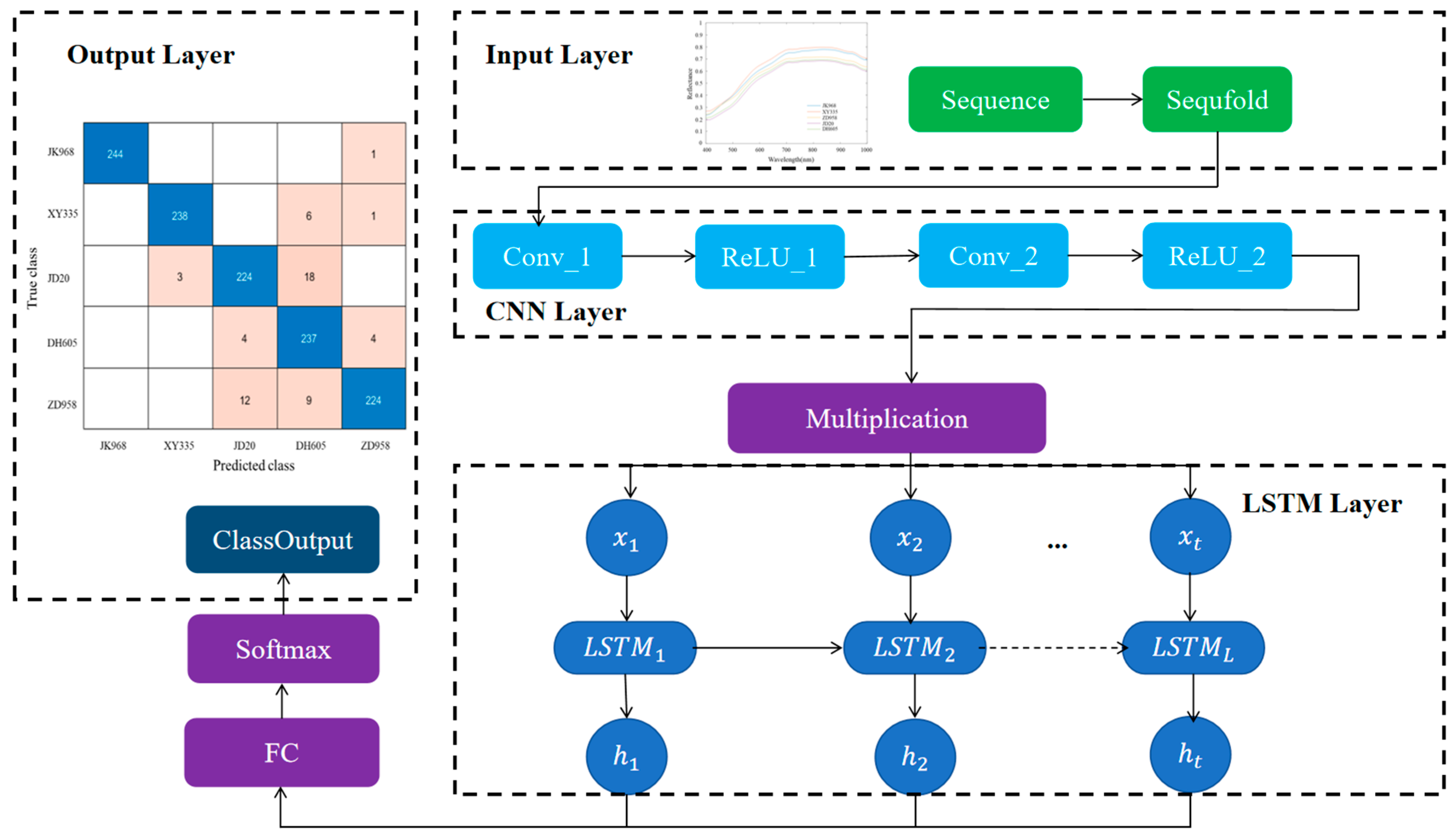
In the CNN-LSTM model, the LSTM component is responsible for training the extracted features, adjusting its parameters via backpropagation to improve both accuracy and stability. The architecture of the CNN-LSTM model is shown in Figure 2. A CNN is a type of feedforward neural network specifically designed to process lattice-like data structures [35]. A CNN uses sliding convolutional filters to automatically extract local features from the data. Convolutional operations, performed by convolutional kernels, replace traditional matrix multiplication, greatly improving computational efficiency. The convolutional layers capture local spatial or temporal patterns in the data, while the pooling layers reduce feature dimensionality. The weight sharing mechanism further minimizes the number of parameters, simplifying the complexity of the model. For time-series data, the output of a one-dimensional convolution can be expressed as follows:
Y = σ ( W · X + b )
where Y represents the extracted features, σ is the sigmoid activation function, W is the weight matrix, X is the time series, and b is the bias vector.
LSTM is an enhanced version of Recurrent Neural Networks (RNNs), specifically designed to overcome the limitations of traditional RNNs in handling long-term dependencies [36]. The core operations of LSTMs involve four key components: the forget gate, the input gate, the cell state update, and the output gate. The forget gate determines how much of the previous memory to retain, while the input gate generates the candidate state for the current time step [37]. The cell state update combines the information from the forget and input gates to modify the memory, and the output gate produces the final output for the current time step. These operations are expressed mathematically by the following set of equations:
f t = σ ( W f [ h t 1 , x t ] + b f )
i t = σ ( W i [ h t 1 , x t ] + b i )
C ~ t = tanh ( W c [ h t 1 , x t ] + b c )
C t = f t C t 1 + i t C ~ t
o t = σ ( W o [ h t 1 , x t ] + b o )
h t = o t tanh ( C t )
where W f , W i , W c , and W o are the weight matrices; b f , b i , b c , and b o are the corresponding bias vectors; t a n h is the hyperbolic tangent function; is used for point multiplication; h t 1 is the output of the previous moment; f t is the retention value; C t 1 is the memory state of the previous moment; i t is the degree of addition of the current moment state; C ~ t is the intermediate state; C t is the current state; o t is the output degree value; h t is the output at the current moment; and x t is the input at the current moment.
The CNN-LSTM hybrid model combined the strengths of both CNN and LSTM, allowing it to capture both local features and long-term sequential dependencies within the data [22]. Specifically, the model consisted of four components: an input layer, a CNN module, an LSTM module, and a classification output layer. The input layer, with a size of [f1,1,1], received the preprocessed sequence data. The CNN module consisted of two convolutional layers: Conv1 with 32 filters of size [1] and Conv2 with 64 filters of size [1]. Each convolutional layer was followed by a ReLU activation function. A global average pooling layer was then applied to reduce the dimensionality of the extracted features. The extracted features were then fed into a 6-hidden-unit LSTM layer, which captured the sequential dependencies in the data. The LSTM module architecture, including the number of LSTM layers and units per layer, was determined based on specific implementation requirements. The classification output layer is a fully connected (Dense) layer employing Softmax activation for multiclass classification, with the number of outputs corresponding to the number of varieties.
During the data preprocessing stage, hyperspectral imaging data were first collected and subsequently processed through denoising, normalization, and standardization procedures to ensure data quality and consistency. Spectral features were then extracted from the preprocessed data to serve as model inputs. The input data dimension was [f1, 1, 1], where f1 represents the number of extracted features, each sequence contains spectral information from a single sample, and the data were typically normalized to the range of 0–1.
During model training, we employed the cross-entropy loss function and the Adam optimizer for weight updates. Training used the Adam optimizer with an initial learning rate of 0.01, halved every 150 epochs to a maximum of 500 epochs. All model developments and data processing were performed using MATLAB R2023a (The MathWorks, Natick, MA, USA). Model performance was evaluated using metrics including accuracy, precision, recall, and F1-score.
This architectural design enables our CNN-LSTM hybrid model to effectively process and analyze hyperspectral imaging data, providing an efficient and accurate approach for automated maize variety identification.

2.6. Model Evaluation

A widely used method to evaluate the performance of a classification algorithm is the confusion matrix, which compares the number of correct predictions to the number of incorrect predictions. The classification accuracy is then calculated as the ratio of correctly predicted samples to the total number of samples. A higher accuracy indicates that the model is good at distinguishing between different maize seed varieties [38].

3. Results and Discussion

3.1. Spectral Analysis

The spectral data for the five maize seed varieties (JK968, XY335, ZD958, JD20, and DH605) in the 400–1000 nm range revealed that while the overall spectral curves were similar, there were discernible differences in reflectance across the varieties (Figure 3). XY335 had a relatively higher reflectance across most of the spectral range, particularly in the near-infrared region. This could suggest that the seeds of XY335 had a denser seed coat, different pigment composition, or a surface structure that reflected more light. JD20 exhibited a lower reflectance compared with other varieties.
The differences in reflectance among five varieties may reflect variations in seed composition, including the seed coat structure, pigment content, or moisture levels. These factors can influence the seed’s interaction with light, affecting how much light is absorbed or reflected across different wavelengths. The 600–700 nm range, in particular, may be related to differences in the amount of chlorophyll or other pigments present in the seed, as this region is known to be sensitive to such compounds [39]. These spectral differences offer valuable insight into the seed characteristics and could potentially be used for the classification of maize seed varieties based on their unique spectral signatures.

3.2. Results of Characteristic Variable Extraction

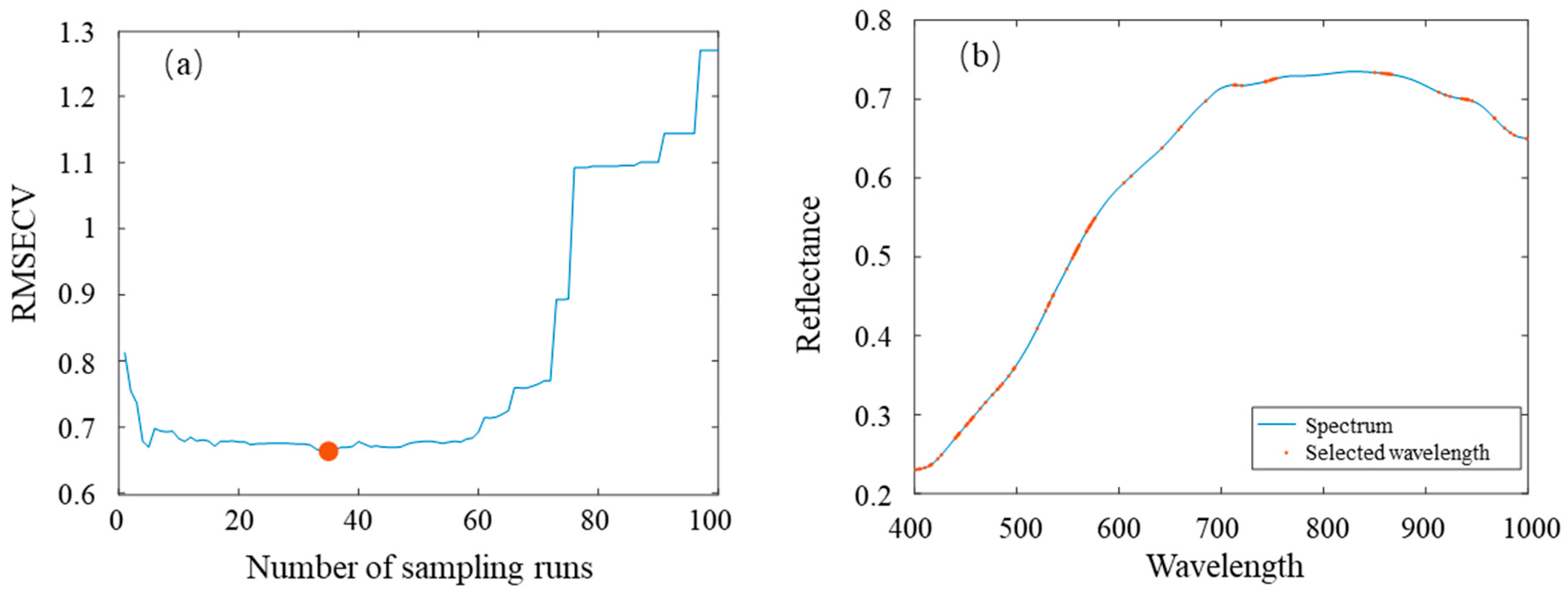
Figure 4 demonstrates the process and results of selecting key feature wavelengths from 774 original wavelength variables using the CARS algorithm. Figure 4a shows the variation in the RMSECV with different sampling iterations, while Figure 4b displays the distribution of the final 100 selected feature wavelengths across the entire spectral curve.
As shown in Figure 4a, the RMSECV value decreased rapidly with the increase in sampling iterations, indicating that the wavelengths eliminated in the initial stages were mostly redundant or noisy variables, which had minimal impact on the model’s capability. Subsequently, the RMSECV entered a stable region, reaching its lowest value at the 38th sampling iteration. This point, marked by a red solid circle in the figure, signified the minimal cross-validation error and optimal performance of the model. After further increasing the number of samples, the RMSECV value noticeably rises, indicating that excessive filtering leads to the loss of useful information, thereby reducing model accuracy. Therefore, the variable set retained after the 38th sampling iteration was determined to be the optimal set of characteristic variables.
The red dots in Figure 4b indicate the 100 key wavelengths retained after CARS, leading to a dimensionality reduction of 87.08% compared with the original full wavelengths. The specific wavelengths are listed in Table 2. The CARS algorithm extracted the most representative spectral bands from high-dimensional data, resulting in a more compact and efficient set of variables and providing a solid foundation for subsequent classification modeling.

3.3. Classification Results of Maize Varieties Based on PLS-DA

The spectral data selected by the CARS algorithm, in conjunction with the indicator matrix representing the variety categories, were utilized as input variables for developing the PLS-DA model (CARS-PLS-DA). The classification results are presented in Table 3. Except for the CARS-PLS-DA model, the PLS-DA model based on the full spectrum was also developed (full-spectrum PLS-DA). It also demonstrates the classification accuracy obtained by directly applying DA to CARS-reduced data using multiple linear regression (MLR), without the PLS step. According to an ANOVA test on these classification results, there was no significant difference among the classification accuracies obtained by the developed models in Table 3 (p < 0.05), demonstrating that the CARS-reduced data did not decrease the classification accuracy statistically.
In this study, the overall classification accuracies for the calibration and prediction sets were 63.27% and 59.10% by CARS-PLS-DA, respectively. The findings further suggested that the classification accuracy exhibited variability among diverse maize seed varieties within both the calibration and prediction sets, thereby indicating that the PLS-DA model’s efficacy was not uniform across all varieties. This variability is particularly evident when comparing the accuracies between the calibration and prediction sets.
For the JK968 variety, the PLS-DA model achieved an accuracy of 70.29% in the calibration set, with a prediction set accuracy of 63.27%. The model demonstrated an effective ability to capture the characteristics of the variety in question by identifying the most significant components. Conversely, the calibration set accuracy for the DH605 variety was found to be comparatively low at 55.75%, yet the model demonstrated superior performance in the prediction set, attaining an accuracy of 69.39%.

3.4. Classification Results of Maize Varieties Based on SVM

Table 4 shows the classification results of the SVM model using three different kernel functions (linear kernel, radial basis function (RBF) kernel, and polynomial kernel) under different hyperparameter settings. The classification accuracies for each kernel function exhibited significant differences between the calibration and prediction sets, reflecting the applicability and effectiveness of different kernel functions in maize seed variety classification.
The linear kernel achieved an accuracy of 99.11% in the calibration set and 93.14% in the prediction set. This result indicated that the linear kernel effectively fitted the training data and demonstrated strong generalization ability, particularly performing well on unseen datasets. It was well suited for classification problems with linearly separable features. The RBF kernel achieved an accuracy of 99.07% in the calibration set, but the accuracy dropped to 81.38% in the prediction set. This change suggested that while the RBF kernel model performed well in the training data, it carried a risk of overfitting, resulting in a weak generalization ability on new data. The polynomial kernel achieved an accuracy of 99.20% in the calibration set, with a prediction set accuracy of 86.45%. Although it performed excellently in the calibration set, its accuracy in the prediction set was lower than the linear kernel, indicating that the polynomial kernel may also exhibited overfitting, especially when dealing with complex nonlinear data.
It can be seen that the best performance in the prediction set was achieved by the linear kernel, with an accuracy of 93.14%. The linear kernel model demonstrated the most stable performance in the prediction set, showing strong generalization ability and making it the optimal kernel choice in this study. Although the RBF and polynomial kernels performed well in the calibration set, their lower accuracies in the prediction set revealed overfitting issues, suggesting that balancing training accuracy with prediction capability need to be considered when selecting kernel functions.

3.5. Classification Results of Maize Varieties Based on ELM

As demonstrated in Figure 5, the classification accuracies in both the calibration and prediction sets were observed to change in accordance with the increase in the number of hidden neurons in the ELM model. It was evident that when the number of hidden neurons was small, the model displayed lower accuracies in both sets. This phenomenon can be attributed to the constrained learning capacity of the neural network, which impeded its capacity to adequately accommodate the data and facilitate precise classifications.
Initially, the accuracy of the prediction set exhibited an incremental rise, reaching approximately 0.47. As the number of hidden neurons increased, the accuracy continued to rise. When the number of hidden neurons reached 100, the prediction set accuracy approached 0.85, reflecting a significant improvement in the model’s learning capacity. However, the accuracy of the calibration set began to plateau, and further increases in the number of hidden neurons led to slower gains in prediction set accuracy. This finding suggests that while the model’s fit to the training set reached its optimal level, its capacity to generalize to unseen data became more constrained. The highest prediction set accuracy of 91.76% was achieved with 290 hidden neurons.

3.6. Classification Results of Maize Varieties Based on CNN-LSTM

The classification results obtained using the CNN-LSTM model demonstrated exceptional performance, attaining 100% accuracy in the classification set and 95.27% accuracy in the prediction set. As illustrated in Figure 6, the performance of the CNN-LSTM model underwent changes throughout the training process. As the number of iterations increased, the accuracy of the model improved steadily, while the loss decreased progressively. This finding suggested that the model effectively learned more relevant features over time, leading to increasingly accurate classification results.
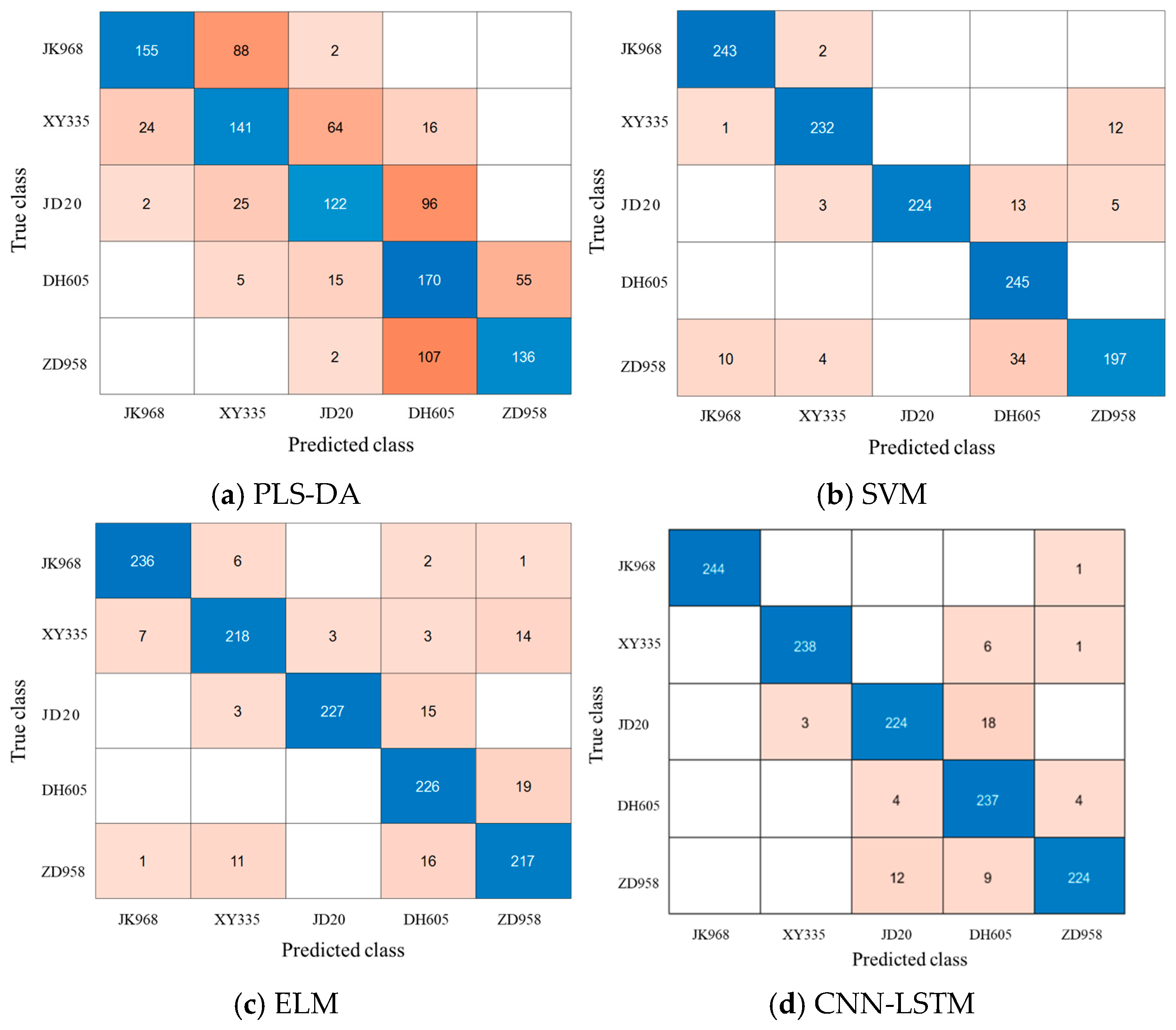
This study utilized a confusion matrix to evaluate the model’s performance in classifying diverse maize varieties. The confusion matrixes for the prediction set were presented for different classicization models (Figure 7), with the x-axis corresponding to the predicted labels and the y-axis representing the true labels. The values along the diagonal indicated the number of samples correctly identified by the classification model. These results indicated that the proposed CNN-LSTM model outperformed traditional machine learning models in maize variety recognition, as more samples were classified correctly, demonstrating its effectiveness in processing spectral data and offering a new direction for future research in similar fields.
In Figure 7d, obtained by CNN-LSTM, it can be seen that the JK968 variety had a higher prediction accuracy in the prediction set, with values on the diagonal close to the number of true labels. For the XY335 variety, the prediction error was small, with only seven samples being misclassified. In contrast, the JD20, DH605, and ZD958 varieties showed higher errors in the classification. The confusion matrix shows that the misclassification of these varieties mainly resulted from their similarity, particularly in their spectral features. Some feature peaks in the spectral curves of these varieties were similar, which increased the difficulty of distinguishing between them for the model.
In addition, Table 5 shows the specific accuracy comparison of CNN-LSTM model with other traditional models in the corn seed variety classification task for each variety. The classification accuracy obtained by PLS-DA was significantly lower compared with those obtained by other models. A comparison of the CNN-LSTM model with traditional machine learning models (PLS-DA, SVM, and ELM) demonstrated an enhancement in prediction accuracy, with improvements of 36.17%, 2.13%, and 3.51%, respectively. This finding underscored the efficiency of the CNN-LSTM model in addressing the prediction challenges inherent in complex datasets.

3.7. Discussion

In this study, a CNN-LSTM model was proposed to classify maize seed varieties, and the experimental results demonstrated that this deep learning model significantly outperformed traditional machine learning methods in spectral analysis [40]. The outstanding performance of the CNN-LSTM model indicated that deep learning approaches possessed stronger capabilities in feature extraction and classification when handling complex spectral data. Specifically, the CNN component effectively extracted local features through convolution operations, while the LSTM component captured long-term dependencies among features, enhancing the model’s ability to process sequential data. This multi-level feature extraction strategy enabled the CNN-LSTM model to better capture subtle spectral differences between maize seed varieties, thereby improving classification accuracy.
Although traditional machine learning models such as PLS-DA, SVM, and ELM also demonstrated reasonable performances, their accuracies were generally lower than that of the CNN-LSTM model, particularly on the prediction set [22]. PLS-DA was effective in reducing data dimensionality and capturing major components; however, its limited ability to model nonlinear relationships led to lower classification performance for certain varieties [41]. The SVM performed well with a linear kernel but showed reduced capability when dealing with nonlinear features. Overfitting was observed when using an RBF kernel, which decreased its generalization performance. The ELM was computationally efficient but sensitive to parameter selection, and its performance declined when an insufficient number of hidden neurons was used.
To address the high dimensionality of spectral data, the CARS algorithm was utilized for feature wavelength selection [42]. By selecting 100 key wavelengths from the full spectral range, CARS significantly reduced data dimensionality while retaining essential spectral information. Compared to traditional feature selection methods, CARS was more effective in extracting representative spectral bands, thus providing a compact and informative foundation for model development. This finding suggested that appropriate feature selection played a crucial role in improving model training efficiency and classification accuracy [43], particularly when handling high-dimensional data.
Despite the excellent performance of the CNN-LSTM model in both calibration and prediction sets, some misclassifications still occurred, particularly among varieties with highly similar spectral features (e.g., JD20, DH605, and ZD958). This phenomenon highlighted the inherent challenges in distinguishing closely related varieties based on spectral data, even when using deep learning models. In this study, only five maize varieties were classified. Future research could expand the dataset to include more varieties to further validate the model’s generalization capabilities across broader application scenarios. Overall, this study confirmed the effectiveness of the CNN-LSTM model for maize variety classification and offered valuable insights into the application of deep learning and feature selection techniques in spectral analysis.

4. Conclusions

The study proposed a novel methodology for the identification of maize varieties, employing a combination of hyperspectral imaging technology and a CNN-LSTM model. Hyperspectral data from five maize varieties were collected, and the raw spectral data were processed using SG smoothing along with SNV preprocessing techniques. In order to further optimize the feature wavelengths, the CARS algorithm was applied, thereby effectively eliminating redundant information and selecting 100 key wavelengths from the original 774. This resulted in an 87% reduction in data dimensionality, thereby minimizing variable collinearity, reducing computational complexity, and enhancing model stability. The integration of the CNN-LSTM module within the model resulted in a recognition accuracy of 95.27% for maize variety classification, thereby demonstrating a substantial enhancement in accuracy over conventional chemometric models such as PLS-DA, SVM, and ELM. The findings indicated that the CNN-LSTM model demonstrated efficacy in the extraction of intricate features from spectral data, exhibiting notable generalization capabilities and superior classification performance. Consequently, the CNN-LSTM model proposed in this study served as a powerful and efficient tool for maize variety identification using hyperspectral imaging.

Author Contributions

Conceptualization, S.F. and Q.L.; methodology, S.F.; software, Q.Z. and D.M.; validation, D.M. and Y.Z.; formal analysis, L.Z. and Q.Z.; investigation, Y.Z. and Q.Z.; resources, S.F. and Q.Z.; data curation, Q.L. and S.F.; writing—original draft preparation, S.F. and Q.Z.; writing—review and editing, Q.Z.; visualization, D.M.; supervision, S.F. and Q.Z.; project administration, Q.Z. and A.W.; funding acquisition, Q.Z. and A.W. All authors have read and agreed to the published version of the manuscript.

Funding

This work was supported by the Natural Science Foundation of Jiangsu Province (Grant No. BK20230548), the National Natural Science Foundation of China (Grant No. 32301712), the Project of Faculty of Agricultural Equipment of Jiangsu University (Grant No. NGXB20240203), and the Project of Jiangsu Province and Education Ministry Co-sponsored Synergistic Innovation Center of Modern Agricultural Equipment (Grant No. XTCX2010).

Data Availability Statement

The original contributions presented in this study are included in the article. Further inquiries can be directed to the corresponding authors.

Conflicts of Interest

The authors declare no conflicts of interest.

References

  1. Zhang, F.; Wang, M.; Zhang, F.; Xiong, Y.; Wang, X.; Ali, S.; Zhang, Y.; Fu, S. Hyperspectral imaging combined with GA-SVM for maize variety identification. Food Sci. Nutr. 2024, 12, 3177–3187. [Google Scholar] [CrossRef] [PubMed]
  2. Sherakhane, M.; Parashivamurthy; Lohithaswa, H.C.; Sinchana Kashyap, G.S.; Gowda, B.; Siddaraju, R.; Keshavareddy, G. Genetic purity assessment of maize hybrid (Zea mays L.) and its parental lines employing SSR markers. J. Adv. Biol. Biotechnol. 2025, 28, 779–785. [Google Scholar] [CrossRef]
  3. Shi, R.; Zhang, H.; Wang, C.; Zhou, Y.; Kang, K.; Luo, B. Data fusion-driven hyperspectral imaging for non-destructive detection of single maize seed vigor. Measurement 2025, 253, 117416. [Google Scholar] [CrossRef]
  4. Zheng, H.; Tang, W.; Yang, T.; Zhou, M.; Guo, C.; Cheng, T.; Cao, W.; Zhu, Y.; Zhang, Y.; Yao, X. Grain protein content phenotyping in rice via hyperspectral imaging technology and a genome-wide association study. Plant Phenomics 2024, 6, 0200. [Google Scholar] [CrossRef]
  5. Fu, L.; Sun, J.; Wang, S.; Xu, M.; Yao, K.; Cao, Y.; Tang, N. Identification of maize seed varieties based on stacked sparse autoencoder and near-infrared hyperspectral imaging technology. J. Food Process Eng. 2022, 45, e14120. [Google Scholar] [CrossRef]
  6. Pang, L.; Wang, J.; Men, S.; Yan, L.; Xiao, J. Hyperspectral imaging coupled with multivariate methods for seed vitality estimation and forecast for Quercus variabilis. Spectroc. Acta Part A-Molec. Biomolec. Spectr. 2021, 245, 118888. [Google Scholar] [CrossRef]
  7. Sun, J.; Nirere, A.; Dusabe, K.D.; Zhong, Y.; Adrien, G. Rapid and nondestructive watermelon (Citrullus lanatus) seed viability detection based on visible near-infrared hyperspectral imaging technology and machine learning algorithms. J. Food Sci. 2024, 89, 4403–4418. [Google Scholar] [CrossRef]
  8. Wang, S.; Sun, J.; Fu, L.; Xu, M.; Tang, N.; Cao, Y.; Yao, K.; Jing, J. Identification of red jujube varieties based on hyperspectral imaging technology combined with CARS-IRIV and SSA-SVM. J. Food Process Eng. 2022, 45, e14137. [Google Scholar] [CrossRef]
  9. Fathi, G.; Mireei, S.A.; Jafari, M.; Sadeghi, M.; Karimmojeni, H.; Nazeri, M. Spatial analysis of hyperspectral images for detecting adulteration levels in bon-sorkh (Allium jesdianum L.) seeds: Application of voting classifiers. Smart Agric. Technol. 2025, 10, 100810. [Google Scholar] [CrossRef]
  10. Cai, Z.; Sun, C.; Zhang, Y.; Shi, R.; Zhang, J.; Zhang, H. Fast detection of the early decay in oranges using visible-LED structured- illumination imaging combined with spiral phase transform and feature-based classification model. Int. J. Agric. Biol. Eng. 2024, 17, 185–192. [Google Scholar] [CrossRef]
  11. Xia, C.; Yang, S.; Huang, M.; Zhu, Q.; Guo, Y.; Qin, J. Maize seed classification using hyperspectral image coupled with multi-linear discriminant analysis. Infrared Phys. Technol. 2019, 103, 103077. [Google Scholar] [CrossRef]
  12. Zhou, Q.; Huang, W.; Fan, S.; Zhao, F.; Liang, D.; Tian, X. Non-destructive discrimination of the variety of sweet maize seeds based on hyperspectral image coupled with wavelength selection algorithm. Infrared Phys. Technol. 2020, 109, 103418. [Google Scholar] [CrossRef]
  13. Jiang, X.; Bu, Y.; Han, L.; Tian, J.; Hu, X.; Zhang, X.; Huang, D.; Luo, H. Rapid nondestructive detecting of wheat varieties and mixing ratio by combining hyperspectral imaging and ensemble learning. Food Control 2023, 150, 109740. [Google Scholar] [CrossRef]
  14. Wang, Y.; Song, S. Detection of sweet corn seed viability based on hyperspectral imaging combined with firefly algorithm optimized deep learning. Front. Plant Sci. 2024, 15, 1361309. [Google Scholar] [CrossRef] [PubMed]
  15. Guo, Z.; Zhang, Y.; Wang, J.; Liu, Y.; Jayan, H.; El-Seedi, H.R.; Alzamora, S.M.; Gomez, P.L.; Zou, X. Detection model transfer of apple soluble solids content based on NIR spectroscopy and deep learning. Comput. Electron. Agric. 2023, 212, 108127. [Google Scholar] [CrossRef]
  16. Donmez, E. Enhancing classification capacity of CNN models with deep feature selection and fusion: A case study on maize seed classification. Data Knowl. Eng. 2022, 141, 102075. [Google Scholar] [CrossRef]
  17. Singh, T.; Garg, N.M.; Iyengar, S.R.S. Nondestructive identification of barley seeds variety using near-infrared hyperspectral imaging coupled with convolutional neural network. J. Food Process Eng. 2021, 44, e13821. [Google Scholar] [CrossRef]
  18. Que, H.; Zhao, X.; Sun, X.; Zhu, Q.; Huang, M. Identification of wheat kernel varieties based on hyperspectral imaging technology and grouped convolutional neural network with feature intervals. Infrared Phys. Technol. 2023, 131, 104653. [Google Scholar] [CrossRef]
  19. Maginga, T.J.; Masabo, E.; Bakunzibake, P.; Kim, K.S.; Nsenga, J. Using wavelet transform and hybrid CNN–LSTM models on VOC & ultrasound IoT sensor data for non-visual maize disease detection. Heliyon 2024, 10, e26647. [Google Scholar] [CrossRef]
  20. Zhou, F.; Hang, R.; Liu, Q.; Yuan, X. Hyperspectral image classification using spectral-spatial LSTMs. Neurocomputing 2019, 328, 39–47. [Google Scholar] [CrossRef]
  21. Liu, Q.; Jiang, X.; Wang, F.; Fan, S.; Zhu, B.; Yan, L.; Chen, Y.; Wei, Y.; Chen, W. Evaluation and process monitoring of jujube hot air drying using hyperspectral imaging technology and deep learning for quality parameters. Food Chem. 2025, 467, 141999. [Google Scholar] [CrossRef]
  22. Wang, Z.; Fan, S.; An, T.; Zhang, C.; Chen, L.; Huang, W. Detection of insect-damaged maize seed using hyperspectral imaging and hybrid 1D-CNN-BiLSTM model. Infrared Phys. Technol. 2024, 137, 105208. [Google Scholar] [CrossRef]
  23. Zhang, L.; Huang, J.; Wei, Y.; Liu, J.; An, D.; Wu, J. Open set maize seed variety classification using hyperspectral imaging coupled with a dual deep SVDD-based incremental learning framework. Expert Syst. Appl. 2023, 234, 121043. [Google Scholar] [CrossRef]
  24. Liu, Q.; Jiang, X.; Wang, F.; Zhu, B.; Yan, L.; Wei, Y.; Chen, Y. Detection of dried jujube from fresh jujube with different variety and maturity after hot air drying based on hyperspectral imaging technology. J. Food Compos. Anal. 2024, 133, 106378. [Google Scholar] [CrossRef]
  25. Wang, Z.; Fan, S.; Wu, J.; Zhang, C.; Xu, F.; Yang, X.; Li, J. Application of long-wave near infrared hyperspectral imaging for determination of moisture content of single maize seed. Spectrochim. Acta. A. Mol. Biomol. Spectrosc. 2021, 254, 119666. [Google Scholar] [CrossRef]
  26. Xu, Y.; Zhang, H.; Zhang, C.; Wu, P.; Li, J.; Xia, Y.; Fan, S. Rapid prediction and visualization of moisture content in single cucumber (Cucumis sativus L.) seed using hyperspectral imaging technology. Infrared Phys. Technol. 2019, 102, 103034. [Google Scholar] [CrossRef]
  27. Wang, Z.; Fan, Y.; Tian, X.; Long, Y.; Huang, W.; Chen, L. Development of a rapid detection method for maize seed purity using a modular high-throughput near-infrared non-destructive testing system. Infrared Phys. Technol. 2025, 148, 105836. [Google Scholar] [CrossRef]
  28. Zhang, N.; Chen, Y.; Zhang, E.; Liu, Z.; Yue, J. Maize quality detection based on MConv-SwinT high-precision model. PLoS ONE 2025, 20, e0312363. [Google Scholar] [CrossRef]
  29. Li, X.; Fu, X.; Li, H. A CARS-SPA-GA feature wavelength selection method based on hyperspectral imaging with potato leaf disease classification. Sensors 2024, 24, 6566. [Google Scholar] [CrossRef]
  30. Lang, F.; Adels, K.; Gaponova, A.; Panchuk, V.; Kirsanov, D.; Monakhova, Y. Fast spectroscopic and multisensor methods for analysis of glucosamine and hyaluronic acid in dietary supplements. Microchem. J. 2024, 207, 112116. [Google Scholar] [CrossRef]
  31. Zhao, S.; Jiao, T.; Adade, S.Y.S.S.; Wang, Z.; Ouyang, Q.; Chen, Q. Digital twin for predicting and controlling food fermentation: A case study of kombucha fermentation. J. Food Eng. 2025, 393, 112467. [Google Scholar] [CrossRef]
  32. Guo, Z.; Zhang, Y.; Xiao, H.; Jayan, H.; Majeed, U.; Ashiagbor, K.; Jiang, S.; Zou, X. Multi-sensor fusion and deep learning for batch monitoring and real-time warning of apple spoilage. Food Control 2025, 172, 111174. [Google Scholar] [CrossRef]
  33. Guo, Z.; Wu, X.; Jayan, H.; Yin, L.; Xue, S.; El-Seedi, H.R.; Zou, X. Recent developments and applications of surface enhanced Raman scattering spectroscopy in safety detection of fruits and vegetables. Food Chem. 2024, 434, 137469. [Google Scholar] [CrossRef]
  34. Li, H.; Hao, Y.; Wu, W.; Tu, K.; Xu, Y.; Zhang, H.; Mao, Y.; Sun, Q. Rapid detection of turtle cracks in corn seed based on reflected and transmitted images combined with deep learning method. Microchem. J. 2024, 201, 110698. [Google Scholar] [CrossRef]
  35. Wongchaisuwat, P.; Chakranon, P.; Yinpin, A.; Onwimol, D.; Wonggasem, K. Rapid maize seed vigor classification using deep learning and hyperspectral imaging techniques. Smart Agric. Technol. 2025, 10, 100820. [Google Scholar] [CrossRef]
  36. Choudhary, K.; Jha, G.K.; Jaiswal, R.; Kumar, R.R. A genetic algorithm optimized hybrid model for agricultural price forecasting based on VMD and LSTM network. Sci. Rep. 2025, 15, 9932. [Google Scholar] [CrossRef] [PubMed]
  37. Simonic, M.; Ficko, M.; Klancnik, S. Predicting corn moisture content in continuous drying systems using LSTM neural networks. Foods 2025, 14, 1051. [Google Scholar] [CrossRef]
  38. Wei, Y.; Liu, Q.; Fan, S.; Jiang, X.; Chen, Y.; Wang, F.; Cao, X.; Yan, L. Development of a predictive model for assessing quality of winter jujube during storage utilizing hyperspectral imaging technology. J. Food Process Eng. 2024, 47, e14688. [Google Scholar] [CrossRef]
  39. Zhu, Y.; Fan, S.; Zuo, M.; Zhang, B.; Zhu, Q.; Kong, J. Discrimination of new and aged seeds based on on-line near-infrared spectroscopy technology combined with machine learning. Foods 2024, 13, 1570. [Google Scholar] [CrossRef]
  40. Xi, Q.; Chen, Q.; Ahmad, W.; Pan, J.; Zhao, S.; Xia, Y.; Ouyang, Q.; Chen, Q. Quantitative analysis and visualization of chemical compositions during shrimp flesh deterioration using hyperspectral imaging: A comparative study of machine learning and deep learning models. Food Chem. 2025, 481, 143997. [Google Scholar] [CrossRef]
  41. Long, Y.; Tang, X.; Fan, S.; Zhang, C.; Zhang, B.; Huang, W. Identification of mould varieties infecting maize kernels based on Raman hyperspectral imaging technique combined with multi-channel residual module convolutional neural network. J. Food Compos. Anal. 2024, 125, 105727. [Google Scholar] [CrossRef]
  42. Liu, L.; Zareef, M.; Wang, Z.; Li, H.; Chen, Q.; Ouyang, Q. Monitoring chlorophyll changes during Tencha processing using portable near-infrared spectroscopy. Food Chem. 2023, 412, 135505. [Google Scholar] [CrossRef] [PubMed]
  43. Li, D.; Park, B.; Kang, R.; Chen, Q.; Ouyang, Q. Quantitative prediction and visualization of matcha color physicochemical indicators using hyperspectral microscope imaging technology. Food Chem. 2024, 163, 110531. [Google Scholar] [CrossRef]
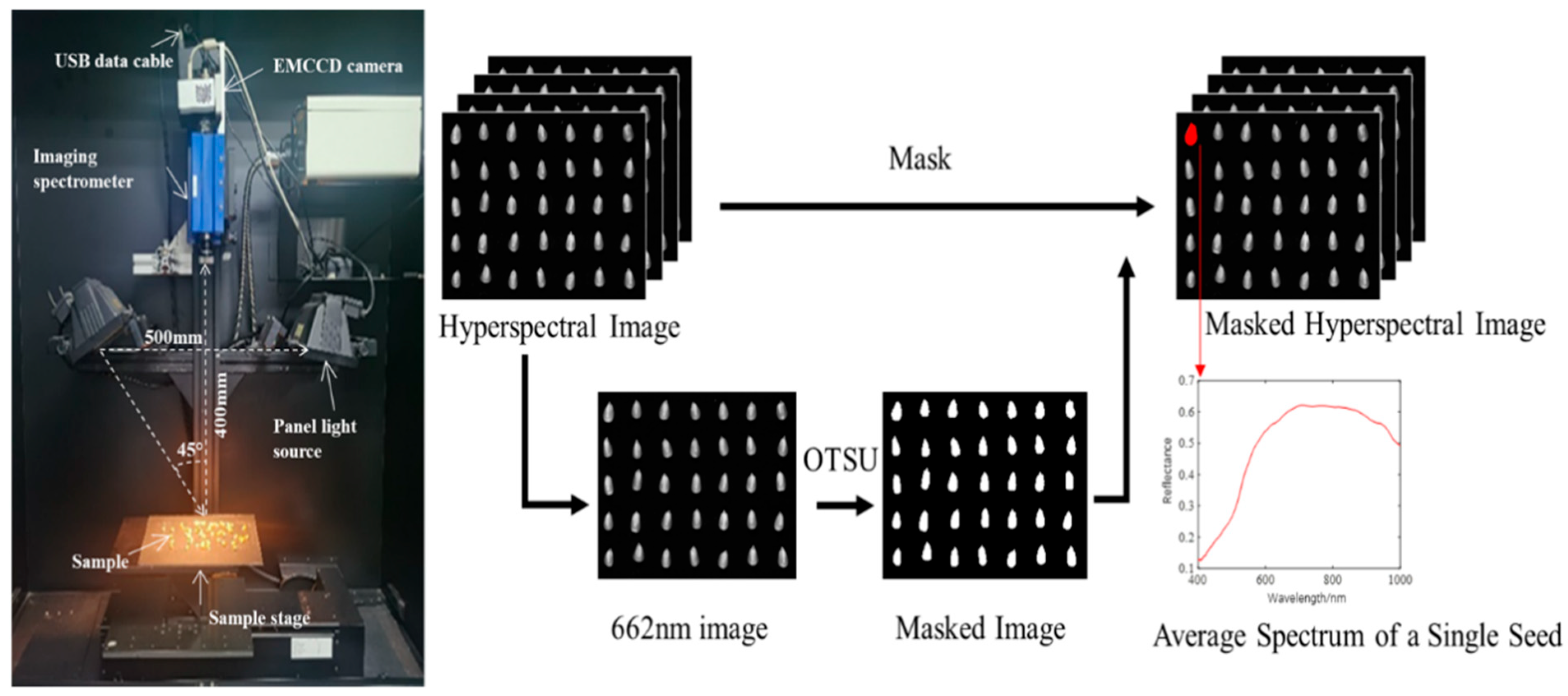
Figure 1. Hyperspectral imaging and data processing flow.
Agronomy 15 01585 g001
Figure 2. CNN-LSTM model architecture diagram.
Agronomy 15 01585 g002
Figure 3. Average spectral curves of seeds from different varieties.
Agronomy 15 01585 g003
Figure 4. Characteristic variable extraction using the CARS algorithm. (a) RMSECV vs. number of sampling runs; (b) distribution of selected wavelengths.
Agronomy 15 01585 g004
Figure 5. Impact of the number of hidden neurons on model classification accuracy.
Agronomy 15 01585 g005
Figure 6. Performance change curves during model training. (a) Accuracy vs. iterations; (b) loss vs. iterations.
Agronomy 15 01585 g006
Figure 7. Confusion matrix for the classification of five maize varieties.
Agronomy 15 01585 g007
Table 1. Distribution of the number of maize seed samples.
Samples SetJK968XY335JD20DH605ZD958
All samples810810810810810
Calibration set565565565565565
Prediction set245245245245245
Table 2. Wavelengths selected based on CARS characteristic selection.
NumbersSelected Wavelength (nm)
100401.3, 404.2, 405.7, 410.1, 414.5, 416.0, 416.8, 422.7, 426.3, 439.7, 440.4, 441.9, 442.7, 443.4, 444.1, 450.1, 451.6, 452.3, 454.6, 455.3, 456.8, 457.5, 464.3, 469.5, 476.2, 480.7, 481.5, 483.7, 486.0, 492.0, 496.5, 497.3, 498.0, 520.0, 528.3, 530.6, 531.4, 532.1, 535.2, 535.9, 548.9, 554.2, 555.7, 556.5, 557.3, 558.0, 558.8, 559.6, 560.3, 561.1, 568.0, 568.8, 570.3, 571.1, 571.8, 572.6, 574.1, 575.7, 576.4, 604.9, 611.8, 642.0, 658.4, 660.7, 684.9, 712.2, 713.8, 714.6, 720.1, 742.8, 743.6, 744.4, 747.6, 748.4, 749.9, 751.5, 753.9, 850.2, 856.6, 858.9, 861.3, 862.9, 864.5, 865.3, 866.9, 912.8, 919.2, 924.0, 935.1, 937.4, 939.0, 940.6, 941.4, 945.4, 966.8, 967.6, 977.1, 982.6, 986.6, 998.5
Table 3. Variety classification results based on PLS-DA and MLR-DA models.
Corn
Varieties
Full-Spectrum PLS-DA ModelCARS-MLR-DA ModelCARS-PLS-DA Model
Calibration Set AccuracyPrediction Set AccuracyCalibration Set AccuracyPrediction Set AccuracyCalibration Set AccuracyPrediction Set Accuracy
JK96868.67%64.48%70.97%61.63%70.29%63.27%
XY33574.33%57.95%64.42%58.37%61.42%57.55%
JD2070.61%53.46%63.36%51.43%64.96%49.80%
DH60573.45%65.30%70.97%71.43%55.75%69.39%
ZD95869.73%66.12%58.05%57.55%64.28%55.51%
Total71.36%61.46%65.56%60.08%63.27%59.10%
Table 4. Classification results of varieties based on SVM.
ParametersParametersCalibration Set AccuracyPrediction Set Accuracy
Linearc, gamma = 10, 0.199.11%93.14%
RBFc, gamma = 4.6, 0.199.07%81.38%
Polyc, gamma = 0.1, 199.20%86.45%
Table 5. Comparison of classification accuracy of different varieties for different models.
Corn VarietiesCNN-LSTM aSVM (Linear Kernel) aELM (Number of Neurons: 290) aPLS-DA b
JK96899.59%99.18%96.33%63.27%
XY33597.14%94.69%88.98%57.55%
JD2091.43%91.43%92.65%49.80%
DH60596.73%100%92.24%69.39%
ZD95891.43%80.41%88.57%55.51%
Different lowercase letters indicate significant differences of classification accuracies (ANOVA test, p < 0.05).
Disclaimer/Publisher’s Note: The statements, opinions and data contained in all publications are solely those of the individual author(s) and contributor(s) and not of MDPI and/or the editor(s). MDPI and/or the editor(s) disclaim responsibility for any injury to people or property resulting from any ideas, methods, instructions or products referred to in the content.