Zonal Estimation of the Earliest Winter Wheat Identification Time in Shandong Province Considering Phenological and Environmental Factors

Abstract

Early-season crop mapping plays a critical role in yield estimation, agricultural management, and policy-making. However, most existing methods assign a uniform earliest identification time across provincial or broader extents, overlooking spatial heterogeneity in crop phenology and environmental conditions. This often results in delayed detection or reduced mapping accuracy. To address this issue, we proposed a zonal-based early-season mapping framework for winter wheat by integrating phenological and environmental factors. Aggregation zones across Shandong Province were delineated using Principal Component Analysis (PCA) based on factors such as start of season, end of season, temperature, slope, and others. On this basis, early-season winter wheat identification was conducted for each zone individually. Training samples were generated using the Time-Weighted Dynamic Time Warping (TWDTW) method. Time-series datasets derived from Sentinel-1/2 imagery (2021–2022) were processed on the Google Earth Engine (GEE) platform, followed by feature selection and classification using the Random Forest (RF) algorithm. Results indicated that Shandong Province was divided into four zones (A–D), with Zone D (southwestern Shandong) achieving the earliest mapping by early December with an overall accuracy (OA) of 97.0%. Other zones reached optimal timing between late December and late January, all with OA above 95%. The zonal strategy improved OA by 3.6% compared to the non-zonal approach, demonstrated a high correlation with official municipal-level statistics (R² = 0.97), and surpassed the ChinaWheat10 and ChinaWheatMap10 datasets in terms of crop differentiation and boundary delineation. Historical validation using 2017–2018 data from Liaocheng City, a prefecture-level city in Shandong Province, achieved an OA of 0.98 and an F₁ score of 0.96, further confirming the temporal robustness of the proposed approach. This zonal strategy significantly enhances the accuracy and timeliness of early-season winter wheat mapping at a large scale.

1. Introduction

Food security remains a critical global concern, increasingly challenged by rapid urbanization, climate change, soil salinization, and arable land degradation, all of which exert mounting pressure on agricultural production [1]. As a major contributor to and beneficiary of global agricultural production and consumption [2], China relies heavily on stable crop yields to safeguard national food security. Winter wheat is one of the most important staple crops, contributing more than 20% to the national grain-sowing area and total yield. The North China Plain functions as the primary zone for its cultivation. Rapid and accurate identification of winter wheat distribution is thus essential for agricultural monitoring, crop management, and structural optimization [3].

Remote sensing has proven to be an effective and economical approach for large-scale crop mapping, owing to its extensive spatial coverage, frequent temporal observations, and inherent objectivity [4]. However, traditional classification approaches typically rely on imagery from the full growing period or from specific phenological stages [5], leading to substantial delays in the availability of crop distribution information—often until harvest or later. For instance, the USDA’s Crop Data Layer (CDL) was generally released five months after harvest, limiting its application for real-time decision-making [6]. To overcome this limitation, early-season crop mapping was proposed to enable the timely identification of crop types during the growing period [7]. This approach supported numerous applications, including disaster response, agricultural insurance, precision farming, yield estimation, and environmental monitoring [8].

Unlike traditional post-season classification, early-season mapping presents several unique challenges. One of the primary issues is the lack of timely training samples, as early-season survey sample collection is labor-intensive, time-consuming, and often delayed beyond the optimal mapping window. To address this, researchers developed a variety of automated sample generation methods. Among them, sample transfer became widely used, whereby early-season samples were generated from historical labeled remote sensing data and applied to current classification tasks [8]. To improve this method’s adaptability to sowing date variations, the Time-Weighted Dynamic Time Warping (TWDTW) technique was incorporated [9]. This method automatically matches historical samples to current crop growth conditions by comparing the similarity of temporal curves and has proven effective in early-season sample generation.

Another challenge stems from the heavy dependence on early-season satellite observations, which are essential for capturing key phenological and spectral traits. However, data quality during this period is often compromised by frequent cloud cover. To mitigate it, time-series interpolation techniques can be employed to reconstruct complete temporal datasets across the crop growth cycle, improving data continuity and usability [10]. Based on the reconstructed time-series feature dataset, feature selection has become a crucial step for improving model performance. It enhances model simplicity, computational efficiency, and classification accuracy. Researchers have typically constructed time-series features spanning the entire growth period to represent spectral responses throughout crop development and to compensate for missing key phenological stages [11]. However, due to the high dimensionality and redundancy in raw features, it was necessary to perform dimensionality reduction before feature ranking [12]. For example, a study in the Huaihe Basin extracted time-series features such as the Normalized Difference Vegetation Index (NDVI), Enhanced Vegetation Index (EVI), Normalized Difference Red Edge Index (NDRDI), and Land Surface Water Index (LSWI), and used the Random Forest (RF) algorithm to evaluate their importance, achieving an early-season accuracy of 91% [13]. Another study in Henan Province selected eight representative spectral indices, including the Land Surface Water Index (LSWI), Green Chlorophyll Vegetation Index (GCVI), Red Edge 2, Inverted Red Edge Chlorophyll Index (IRECI), and others, further improving classification performance [14].

Despite considerable progress in early-season crop mapping, large-scale applications remain challenging due to spatial heterogeneity and environmental variability. In Shandong Province, several studies have reported an underestimation of winter wheat distribution during the overwintering period [5,15], primarily attributed to inconsistent phenological development driven by topographic and climatic differences. In warmer and wetter zones, winter wheat resumes growth earlier, while in colder areas with limited sunlight, its growth remains dormant for extended periods. Consequently, early detection requires zone-specific adaptation to phenological and environmental differences. To mitigate spatial inconsistency, some studies incorporated phenological information into mapping frameworks. For example, rice distribution in Northeast Asia was effectively mapped using flood signal phenology combined with vegetation indices [16]. However, environmental factors such as rainfall, temperature, and elevation exhibited substantial spatial variability, making it challenging to fully capture zonal differences based solely on phenological features. Thus, zone-specific threshold adjustments were still necessary to maintain classification stability across diverse zones [17].

Subdividing the study area into finer zones was recognized as an effective strategy to enhance zonal adaptability. Systems such as Agroecological Zones (AEZs) and Agricultural Climatic Zones (ACZs) were widely adopted to support zonal classification and improve large-scale mapping accuracy. For instance, the classification accuracy of winter wheat significantly improved after Jiangsu Province was divided into four AEZs and mapped separately [18]. Nevertheless, predefined zones often failed to reflect real-time planting conditions within a given year, limiting their effectiveness for early-season mapping. Therefore, future zoning strategies require dynamic integration of phenological and environmental information to improve robustness and adaptability.

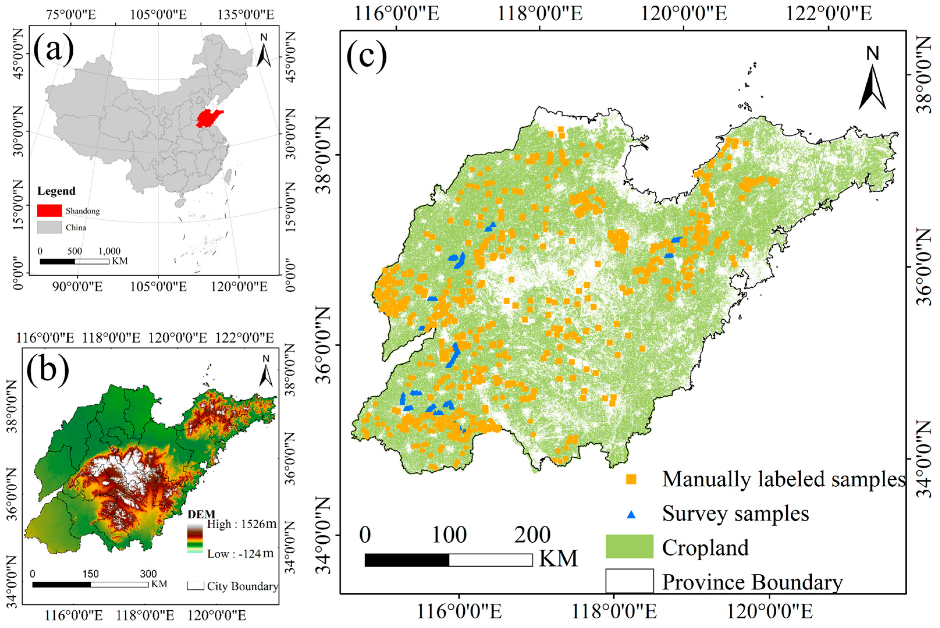
To tackle these challenges, this study proposes a zonal-based early-season mapping approach that integrates phenological and environmental factors. Zone-specific optimal identification times in Shandong Province are determined using Sentinel-1/2 time-series data processed on the Google Earth Engine (GEE) platform. This study aims to (1) construct and assess an integrated approach to enhance both the timeliness and accuracy of large-area winter wheat mapping at early growth periods; (2) identify the earliest feasible identification time for winter wheat within each defined zone; and (3) develop zone-specific classification strategies that account for environmental heterogeneity.

2. Materials

2.1. Study Area

Shandong Province, located in the lower reaches of the Yellow River, extends from 34°23′ N to 38°17′ N and 114°48′ E to 122°42′ E. As a prominent agricultural zone in eastern China, it lies within the North China Plain and is characterized by a warm temperate monsoon climate, featuring hot and rainy summers as well as cold and dry winters (Figure 1a). These climatic conditions, coupled with fertile soil, provide an optimal environment for agricultural production. The central part of Shandong Province features mountainous landscapes, whereas the southwest and northwest are mainly flat and low in elevation. In contrast, the eastern area is dominated by gently rolling hills (Figure 1b).

In 2021, the arable land of Shandong Province reached 64,000 km², representing 40.5% of the provincial territory, highlighting its importance as a major grain-producing zone. Winter wheat had a sown area of 2.357 million ha in 2021, comprising 16.95% of the national winter wheat cultivation [19]. As China’s second-largest winter wheat-producing province, Shandong is crucial to maintaining national food security.

In Shandong, winter wheat typically grows over a period of 220 to 270 days. Sowing occurs from September to October, followed by dormancy beginning in December. As temperatures rise, growth resumes between February and March. The jointing stage usually starts in early April, transitions into the heading phase from mid-April to May, and the crop is generally harvested by June.

2.2. Data and Preprocessing

2.2.1. Remote Sensing Imageries

This study utilized 1428 Sentinel-2 Multi Spectral Instrument (MSI) Top-of-Atmosphere (TOA) reflectance images acquired from the GEE platform, spanning the winter wheat-growing period in Shandong Province from 10 October 2021 to 10 June 2022. Additionally, 464 Sentinel-2 images were acquired for Liaocheng City during the 2017–2018 winter wheat-growing period [20]. Sentinel-2 provided 13 spectral bands with a maximum spatial resolution of 10 m and a temporal resolution of 5 days. During the 2021–2022 winter wheat-growing period, pixels with cloud cover greater than 30%, as indicated by the QA60 band, were excluded, and only cloud-free or low-cloud images (with cloud cover below 30%) were retained for further analysis. These valid images provided sufficient spatial and temporal coverage for the study area.

To mitigate temporal discontinuities caused by orbital differences, the Sentinel-2 data were aggregated into 10-day intervals using maximum value compositing. A Savitzky–Golay (SG) filter with a 70-day moving window and a third-order polynomial function was subsequently employed to smooth the time series, generating a dataset with 10-day temporal intervals.

We also acquired Sentinel-1 Ground Range Detected (GRD) images during the winter wheat-growing period, including 392 scenes across Shandong Province from 2021 to 2022 and 98 scenes within Liaocheng City from 2017 to 2018. The dataset comprised vertical transmit/vertical receive (VV) and vertical transmit/horizontal receive (VH) polarization modes acquired in Interferometric Wide (IW) swath mode. Sentinel-1 imagery featured a spatial resolution of 10 m and a temporal resolution of 6 days. The preprocessing workflow included the elimination of thermal noise, application of radiometric calibration, and execution of terrain correction. Speckle suppression was achieved using a refined Lee filter with a 7 × 7 kernel. The processed SAR images were then resampled to a 10-day interval to align with the Sentinel-2 time series, ensuring temporal consistency in the integration of multi-source remote sensing datasets.

2.2.2. Auxiliary Data

This study employed phenological features and environmental factors jointly to generate zones. Phenological features were obtained by fitting time-series curves using the TIMESAT (version 3.3) software based on the MOD13A1.061 Terra 16-Day 500 m Global Vegetation Indices dataset provided by the GEE platform [21]. Environmental factors, including average temperature, evapotranspiration, and precipitation during the winter wheat-growing period (October to the following June), as well as terrain slope, were extracted from the following datasets. Specifically, the temperature, evapotranspiration, and precipitation data were obtained from the National Tibetan Plateau Data Center (https://data.tpdc.ac.cn/, accessed on 1 October 2024), while the slope was derived from the digital elevation model (DEM) provided by the United States Geological Survey (https://earthexplorer.usgs.gov/, accessed on 1 October 2024). All datasets were reprojected and resampled to 1 km resolution to ensure spatial alignment and positional consistency.

Cropland data from the global 10 m land cover product dataset “ESA/WorldCover/v200” released by the European Space Agency (ESA) in 2021 and winter wheat planting area official statistics from the Shandong Provincial Bureau of Statistics (http://tjj.shandong.gov.cn/tjnj/nj2021/indexch.htm, accessed on 1 October 2024) for Shandong Province were collected for masking the cropland and comparison analysis, respectively.

To enable the automatic acquisition of winter wheat training samples, we collected historical winter wheat datasets, including ChinaWheatMap10 [22], ChinaWheat10 [23], and the 30 m winter wheat distribution map of 11 provinces in China [24], from which samples were extracted to serve as reference data for current-season sample selection.

2.2.3. Sample Dataset

Over the course of the 2021–2022 winter wheat-growing period, the research team systematically collected survey samples using handheld GPS devices, encompassing winter wheat and other crop types. To improve the reliability and representativeness of the sample dataset, all field survey samples were carefully validated using Google Earth high-resolution imagery. In addition, supplementary winter wheat and non-winter wheat samples were manually labeled through visual interpretation based on high-resolution images available from Google Earth (Figure 1c). The integrated set of survey samples and manually labeled samples was subsequently used to construct standard VH time-series curves, which supported the automatic sample generation process and served as validation samples for evaluating the accuracy of winter wheat classification. The collected validation samples are presented in

Table 1. The number of validation samples in 2021.

Sample Types	Winter Wheat	Non-Winter Wheat	Total
Survey samples	134	109	243
Manually labeled samples	225	459	684
Total	359	568	927

.

3. Methods

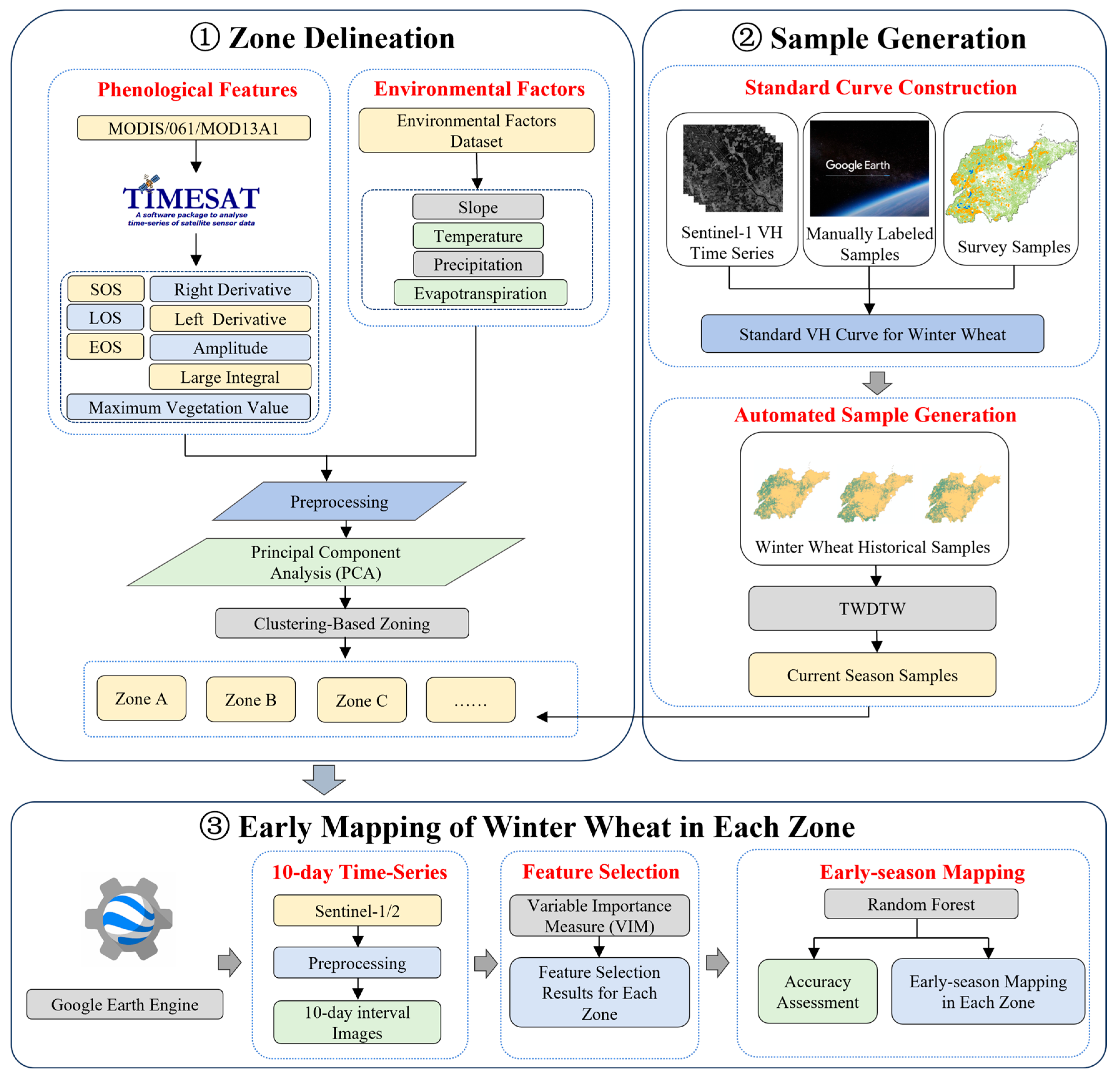
The flowchart is illustrated in Figure 2. The primary objective of the study was to accurately determine the earliest identification time of winter wheat across different zones in Shandong Province, following three main steps:

(1) Zoning Shandong Province based on a comprehensive analysis of phenological features and environmental factors.

(2) Automatically generating current-season training samples for winter wheat and non-winter wheat using the TWDTW method.

(3) Selecting optimal features for each zone and employing the Random Forest classifier to determine the earliest identification time of winter wheat.

3.1. Clustering Zone Generation Based on Phenological and Environmental Factors

3.1.1. Phenological and Environmental Factors Preparation

In this study, zonal delineation across the study area was based on phenological features and environmental factors, with detailed descriptions provided in

Table 2. Selected phenological features and environmental factors in the study.

	Factors	Implication
Phenological Features	SOS (Start of Season)	The time when plant growth begins, marked by an initial rise in the vegetation index.
	Amplitude	The difference between the peak and baseline vegetation index, indicating growth intensity.
	EOS (End of Season)	The time when the vegetation index starts decreasing, marking dormancy onset.
	LOS (Length of Season)	The total vegetation index accumulated over the season, reflecting productivity.
	LI (Large Integral)	The cumulative sum of the vegetation index over the growing season, reflecting total vegetation productivity.
	MVV (Maximum Value of Vegetation)	The highest vegetation index value, representing peak growth.
	Left Derivative	The rate of vegetation increase during early growth indicates the transition speed.
	Right Derivative	The rate of vegetation decline, indicating the shift to dormancy.
Environmental Factors	Precipitation	A key water source for vegetation, affecting soil moisture and crop growth.
	Temperature	Influences plant growth rate; extreme temperatures can hinder crops.
	Evapotranspiration	Measures water loss from soil and plants, affecting moisture balance.
	Slope	Describes land steepness, impacting water runoff, erosion, and soil moisture.

. To avoid multicollinearity among these factors, the Spearman correlation coefficients were first calculated, and variables with a correlation greater than 0.9 were excluded [25]. Specifically, amplitude and maximum vegetation value (MVV) exhibited a high degree of correlation, and thus, MVV was removed.

Secondly, Principal Component Analysis (PCA) was employed to condense the dimensionality of the selected phenological and environmental factors. Prior to analysis, all variables were standardized using Z-score normalization to eliminate the influence of scale differences among indicators, as defined by the following formula:

$$x^{\prime }={\displaystyle \frac{x-\overline{x}}{\sigma }}$$

(1)

where $x^{\prime }$ refers to the standardized form of the variable, computed as the deviation from the mean $\overline{x}$, normalized by the standard deviation $\sigma$.

Subsequently, principal components were extracted, and an orthogonal rotation was applied to optimize the loading matrix structure, thereby enhancing the interpretability of each principal component. In accordance with the commonly used eigenvalue criterion, only components with eigenvalues exceeding 1 were preserved [26], as these accounted for the majority of the variance within the dataset. Each principal component was expressed as a linear combination of standardized variables, formulated as

$$F_i=a_1{x}_1+a_2{x}_2+\cdots +a_n{x}_n$$

(2)

where $F_i$ represents the $i$-th principal component, $a_1,a_2,...,a_n$ are the corresponding coefficients, and $x_1,x_2,...,x_n$ represent the standardized indicator values.

Through this approach, complex phenological and environmental factors were transformed into a limited number of comprehensive principal components. This not only reduced data dimensionality, but also more clearly revealed the dominant variations among indicators and their internal relationships.

3.1.2. Zone Delineation Using K-Means Clustering Method

In this study, the K-means clustering algorithm was applied to group and analyze the composite indicators obtained through PCA. As a widely adopted unsupervised learning method, K-means delineates spatially homogeneous zones by assigning each sample to the nearest cluster centroid, thereby minimizing the total within-cluster sum of squares.

This clustering approach effectively delineates zones with similar feature characteristics, enabling a reduction in internal heterogeneity across large-scale research areas. K-means was selected not only for its computational efficiency and scalability but also due to its unsupervised nature, which avoids reliance on manually selected training samples and minimizes human subjectivity. Instead, it clusters samples based solely on their intrinsic feature separability. Similar strategies have been successfully employed in previous studies involving time-series remote sensing data for crop phenology and zonal mapping, further demonstrating the method’s robustness and suitability for large-scale agricultural applications [25,27].

During the clustering process, the similarity between samples was quantified using the Euclidean distance, as defined by the following formula:

$$d\left(x,y\right)=\sqrt{\sum _{i=1}^n{\left(x_i-y_i\right)}^2}$$

(3)

where $d\left(x,y\right)$ quantifies the dissimilarity between two samples $x$ and $y$, $x_i$ and $y_i$ represent the values of the $i$-th feature for each sample, and $n$ is the total number of features. Based on this distance metric, each sample was iteratively assigned to the closest cluster center.

To determine the optimal number of clusters, both the Elbow Method and the Silhouette Coefficient were adopted. The Elbow Method involved plotting the ratio of the between-cluster sum of squares (BSS) to total sum of squares (TSS) across varying values of $k$, and identifying the point at which the rate of increase in this ratio began to level off. The ratio was computed using the following formula:

$${\displaystyle \frac{\mathrm{BSS}}{\mathrm{TSS}}}={\displaystyle \frac{{\sum }_{j=1}^k{n}_j|{\mu }_j-\overline{x}{|}^2}{{\sum }_{i=1}^N|x_i-\overline{x}{|}^2}}$$

(4)

where $N$ represents the total sample size, $k$ represents the number of clusters, $x_i$ is the feature vector of the $i$th sample, $\overline{x}$ denotes the overall mean, ${\overline{\mu }}_j$ is the centroid of cluster $j$, and $n_j$ indicates the number of samples in the cluster [28].

Moreover, the Silhouette Coefficient was employed to assess the clustering quality by simultaneously considering the cohesion within clusters and the separation between different clusters. It provides an effective metric for evaluating the overall clustering structure, and has been widely applied in ecological and remote sensing studies due to its balance between intra-cluster compactness and inter-cluster distinctiveness [25]. It was calculated as

$$S\left(k\right)={\displaystyle \frac{b\left(k\right)-a\left(k\right)}{\max \left(a\left(k\right),b\left(k\right)\right)}}$$

(5)

where $a\left(k\right)$ denotes the mean distance between sample $k$ and all other members of the same cluster, whereas $b\left(k\right)$ refers to the average distance between sample $k$ and the samples in the closest adjacent cluster. The coefficient varied between −1 and 1, with values approaching 1 indicating stronger and more distinct clustering.

Finally, the results of both evaluation metrics were jointly considered to determine the optimal number of clusters. This ensured that the final zonal delineation achieved both internal homogeneity and external distinctiveness across the delineated zones.

3.2. Automated Sample Generation Using the TWDTW Method

To obtain representative winter wheat training samples with strong adaptability and robustness, winter wheat pixels were first extracted from historical datasets corresponding to 2018, 2019 and 2020, and then their spatial intersection was calculated. To further refine the sample quality, an area-based filtering step was subsequently applied. Specifically, winter wheat patches were ranked by area, and the smallest 50% were excluded. This allowed the retention of only relatively large and spatially consistent zones, from which training samples were selected.

Subsequently, a standard winter wheat time-series curve was constructed based on both survey samples and manually labeled samples. The TWDTW algorithm was then applied to calculate the TWDTW distance between candidate pixels and the standard curve. Pixels with TWDTW distances below a predefined threshold were selected as training samples.

The selection of an appropriate input variable is critical to the effectiveness of TWDTW in sample generation. Common vegetation indices like NDVI and EVI exhibited constrained effectiveness in differentiating winter wheat from other co-occurring winter crops. In contrast, a significant discrepancy in VH backscatter coefficients between winter wheat and other winter crops in Shandong Province was reported, indicating the potential of the VH band to enhance class separability [20]. Therefore, VH time-series data were employed as inputs to the TWDTW algorithm to facilitate the automated extraction of training samples.

3.3. Winter Wheat Early-Season Mapping

3.3.1. Feature Selection

This study integrated both spectral and radar features to enhance the discrimination among crop types and mitigate the adverse effects caused by spectral similarity on classification performance. Spectral features captured the physiological and biochemical characteristics of vegetation, whereas radar features provided complementary information related to surface structure and backscattering properties. The fusion of these heterogeneous data sources significantly improved the robustness and accuracy of crop classification.

Specifically, spectral features were derived from ten multispectral bands of Sentinel-2 imagery, alongside vegetation indices that reflect crop growth conditions [29]. Radar features included the VV and VH polarization bands extracted from Sentinel-1 data [30], which are sensitive to surface roughness and structural variations. The detailed list of spectral bands and vegetation indices used in this study is provided in

Table 3. Summary of the feature types employed in the study.

Feature Types	Features	Description
Spectral features	Sentinel-2 bands	${\rho }_{\mathrm{blue}}, {\rho }_{\mathrm{green}}{, \rho }_{\mathrm{red}}, {\rho }_{\mathrm{red}\_\mathrm{edge}1}, {\rho }_{\mathrm{red}\_\mathrm{edge}2}, {\rho }_{\mathrm{red}\_\mathrm{edge}3}, {\rho }_{\mathrm{red}\_\mathrm{edge}4}, {\rho }_{\mathrm{nir}}, {\rho }_{\mathrm{swir}1}, {\rho }_{\mathrm{swir}2}$
	Enhanced Vegetation Index (EVI) [31]	$\begin{array}{c}\mathrm{E}\mathrm{V}\mathrm{I}=2.5\times {\displaystyle \frac{{\rho }_{\mathrm{nir}}-{\rho }_{\mathrm{red}}}{{\rho }_{\mathrm{nir}}+6\times {\rho }_{\mathrm{red}}-7.5\times {\rho }_{\mathrm{blue}}+1}}\end{array}$
	Land Surface Water Index (LSWI) [32]	$\begin{array}{c}\mathrm{L}\mathrm{S}\mathrm{W}\mathrm{I}={\displaystyle \frac{{\rho }_{\mathrm{nir}}-{\rho }_{\mathrm{swir}1}}{{\rho }_{\mathrm{nir}}+{\rho }_{\mathrm{swir}1}}}\end{array}$
	Normalized Difference Vegetation Index (NDVI) [33]	$\begin{array}{c}\mathrm{N}\mathrm{D}\mathrm{V}\mathrm{I}={\displaystyle \frac{{\rho }_{\mathrm{nir}}-{\rho }_{\mathrm{red}}}{{\rho }_{\mathrm{nir}}+{\rho }_{\mathrm{red}}}}\end{array}$
	Green Chlorophyll Vegetation Index (GCVI) [34]	$\begin{array}{c}\mathrm{G}\mathrm{C}\mathrm{V}\mathrm{I}={\displaystyle \frac{{\rho }_{\mathrm{nir}}}{{\rho }_{\mathrm{green}}}}-1\end{array}$
	Inverted Red-Edge Chlorophyll Index (IRECI) [35]	$\begin{array}{c}\mathrm{I}\mathrm{R}\mathrm{E}\mathrm{C}\mathrm{I}={\displaystyle \frac{{\rho }_{\mathrm{nir}}-{\rho }_{\mathrm{red}}}{{\rho }_{\mathrm{red}\_\mathrm{edge}1}+1}}\end{array}$
	Green Normalized Difference Vegetation Index (GNDVI) [36]	$\begin{array}{c}\mathrm{G}\mathrm{N}\mathrm{D}\mathrm{V}\mathrm{I}={\displaystyle \frac{{\rho }_{\mathrm{nir}}-{\rho }_{\mathrm{green}}}{{\rho }_{\mathrm{nir}}+{\rho }_{\mathrm{green}}}}\end{array}$
	Soil-Adjusted Vegetation Index (SAVI) [37]	$\begin{array}{c}\mathrm{S}\mathrm{A}\mathrm{V}\mathrm{I}={\displaystyle \frac{{(\rho }_{\mathrm{nir}}-{\rho }_{\mathrm{red}})}{{\rho }_{\mathrm{nir}}+{\rho }_{\mathrm{red}}+L}}\times \left(1\times L\right)\end{array}$
Radar features	Backscattering coefficient	$\mathrm{VV}, \mathrm{VH}$

.

To identify the most discriminative features for classification within each zone, the RF algorithm was employed to calculate the Variable Importance Measure (VIM) scores (Section 3.3.2). An ensemble of decision trees was constructed, and the averaged feature importance scores were used to identify the most relevant variables, thereby optimizing the overall classification performance.

3.3.2. Winter Wheat Early-Season Mapping and Accuracy Assessment

The RF algorithm was utilized in this study to facilitate the early-season identification of winter wheat. RF has been widely applied to land cover monitoring tasks on the GEE platform [38], including dynamic land cover mapping, detection of croplands and irrigated areas, and crop type classification [39]. Within the framework of ensemble learning, RF enhanced model diversity and reduced generalization error by incorporating bootstrap aggregation (bagging) and random feature subset selection. Moreover, it allowed for the evaluation of variable importance when determining class labels. During the classification process, final outputs were determined by majority voting across all decision trees. Previous studies have demonstrated that RF outperformed several traditional classifiers, including maximum likelihood classification and shallow neural networks, in terms of robustness, accuracy, and computational efficiency [12,40]. Given its strong capability in handling high-dimensional data and its robustness to collinearity and redundancy, RF was well suited to the needs of this study.

The number of trees in the RF was set to 100, and the minimum number of samples per leaf node was set to 10, while all remaining hyperparameters were kept at their default values.

Early-season winter wheat mapping was conducted for each zone based on the optimal strategy identified for that specific zone. Classification performance was assessed based on confusion matrices, from which evaluation metrics including overall accuracy (OA), user’s accuracy (UA), producer’s accuracy (PA), and the F₁ score were derived.

$$F_1=2\times {\displaystyle \frac{PA\times UA}{PA+UA}}$$

(6)

4. Results

4.1. Clustering Zone Results and Analysis

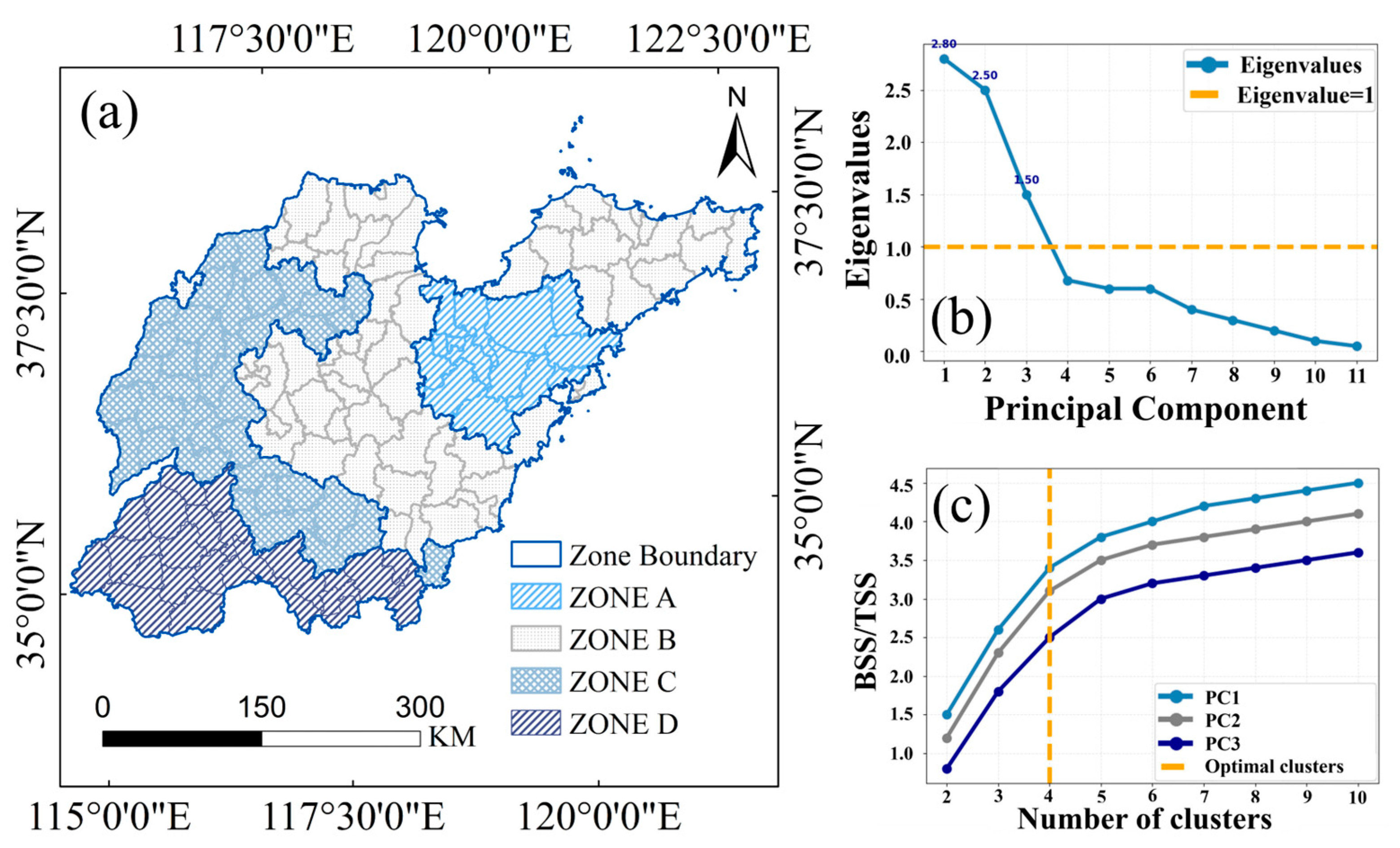
In this study, a total of eleven principal components were extracted through PCA. The eigenvalues of the first three principal components were 2.80, 2.50, and 1.50, respectively, cumulatively explaining 86.9% of the total variance (PC1: 40.5%; PC2: 27.7%; PC3: 18.7%). The eigenvalues of these components were significantly greater than 1, whereas those of subsequent components declined rapidly and remained stable, indicating their relatively minor contribution to overall variability (Figure 3b).

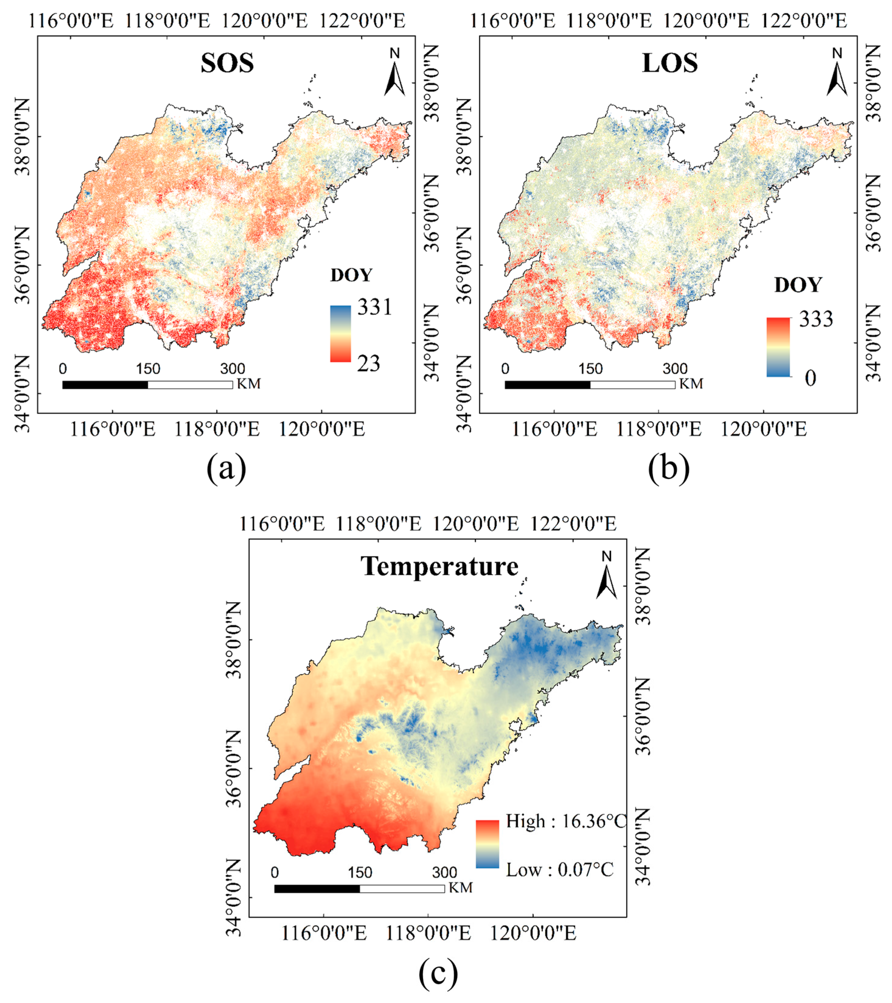
PC1 exhibited a strong correlation with the SOS. The spatial distribution of the SOS ranged from 23 to 331 days across the study area, with earlier onset observed in southern Shandong and later dates in northern and mountainous zones (Figure 4a). PC2 was closely associated with temperature during the growing period. Temperature values ranged from 0.07 °C to 16.36 °C, with higher temperatures mainly concentrated in the southwestern part of the province (Figure 4c). PC3 was strongly correlated with the LOS, which revealed substantial zonal differences in crop development periods. In particular, southern areas experienced longer growing seasons due to warmer climatic conditions (Figure 4b).

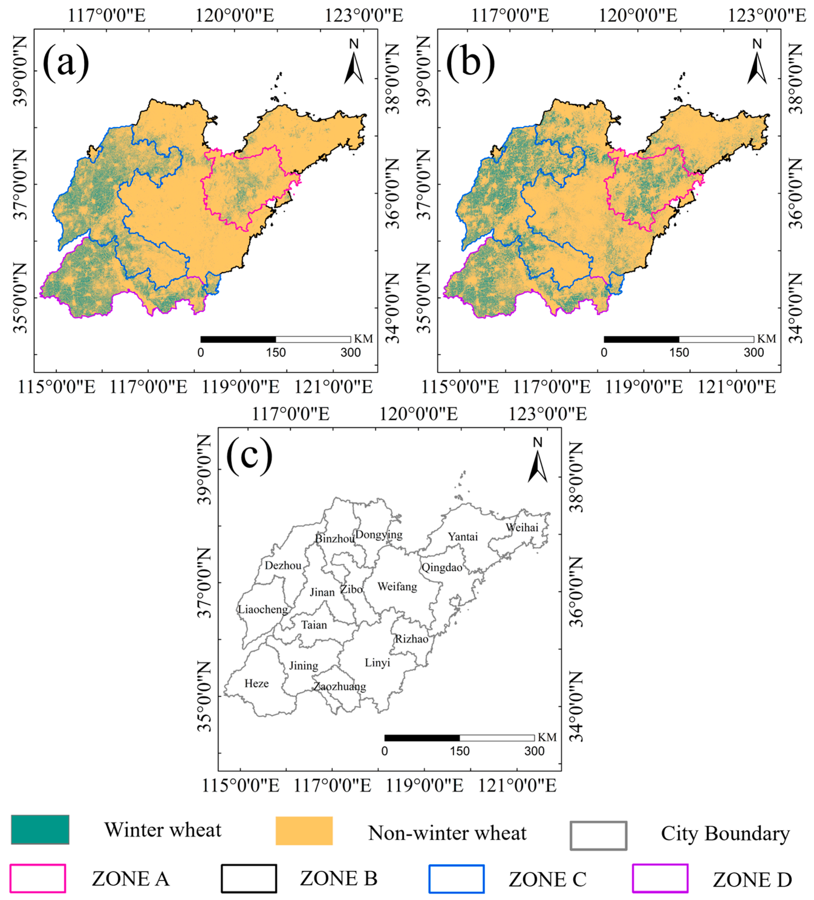
The optimal number of clusters was determined as four using the Elbow Method, which involved evaluating the total within-cluster sum of squares alongside the explanatory power of principal components under varying cluster configurations (Figure 3). The final clustering results delineated the study area into four distinct zones (Zone A, Zone B, Zone C, and Zone D), each exhibiting unique phenological and environmental characteristics (Figure 3a).

Zone A (mainly encompassing parts of Weifang and Qingdao) was characterized by early greening and moderate thermal accumulation, creating favorable conditions for winter wheat cultivation. Zone B (including Yantai, Dongying, and portions of Weifang and Zibo) featured higher elevation, resulting in a noticeable delay in phenological development. Zone C (primarily including Liaocheng and parts of Dezhou and Jining) displayed intermediate phenological and meteorological conditions. Zone D (covering Heze and parts of Jining and Zaozhuang) had SOS values predominantly between 45 and 100 days, with an average of 64 days, indicating a significantly earlier growing season onset compared to other zones. This zone’s distinctiveness lay in its early SOS combined with suitable thermal conditions, making its phenological profile notably different from the rest.

4.2. Training Sample Generation

To train zone-specific RF classification models for early-season winter wheat mapping, high-confidence training samples were generated using the TWDTW algorithm with historical data. In this study, the distribution of training samples was relatively balanced, with sufficient quantity and category representation to support reliable model training in each zone.

Using the TWDTW algorithm, the similarity between the standard VH time-series curve of winter wheat for each zone and the corresponding historical sample curves was computed. To determine the optimal threshold, the Otsu automatic thresholding method was applied, resulting in an average threshold value of 1.73 for sample generation across the four zones. The winter wheat and non-winter wheat samples selected under this threshold were then used for zone-specific crop classification training.

A total of 2423 winter wheat samples and 1022 non-winter wheat samples were collected, resulting in a combined dataset of 3445 samples. Among all zones, Zone C contributed the largest number of training samples, with 1415 in total—comprising 956 winter wheat and 459 non-winter wheat samples. This was primarily due to the extensive and representative winter wheat cultivation areas in this region, which enabled efficient and effective sample extraction. Zone D followed with 1009 samples, while Zones B and A contributed 719 and 302 samples, respectively (

Table 4. The number of training samples in each zone in 2021.

	Winter Wheat	Non-Winter Wheat	Total
Zone A	196	106	302
Zone B	546	173	719
Zone C	956	459	1415
Zone D	725	284	1009
Total	2423	1022	3445

).

4.3. Winter Wheat Early-Season Mapping Results

4.3.1. Feature Selection Results

As illustrated in Figure 5, several spectral bands and vegetation indices—particularly SWIR1, EVI, NDVI, VH, and GCVI—consistently exhibited high VIMs across all four delineated zones, indicating their strong and stable relevance for early-season winter wheat identification.

Despite this overall consistency, notable differences were observed in the importance rankings of features among the individual zones, reflecting the spatial heterogeneity in remote sensing responses. Specifically, the top six features in Zone A were RED, EVI, RE2, SWIR1, SAVI, and VH, while Zone B emphasized EVI, NDVI, VH, IRECI, SWIR1, and GCVI. In Zone C, the most important features included SWIR1, GCVI, RED, VH, NDVI, and GNDVI. For Zone D, SWIR1, VH, NDVI, GCVI, EVI, and RE3 were most relevant.

The observed discrepancies in feature importance can be explained by zonal agroecological variability, such as sowing dates, topographic conditions, and accumulated thermal time across zones. Therefore, the development of zone-specific feature selection strategies is essential to accommodate zonal variability in crop growth patterns and spectral characteristics, ultimately enhancing classification accuracy and generalization. Based on these insights, the top six features in each zone were selected to support subsequent classification tasks.

4.3.2. Zonal Early-Season Mapping Results and Analysis

Based on the optimized feature combinations and zone-specific RF, winter wheat classification was conducted across the four delineated zones. The classification model was trained using samples generated through TWDTW and Otsu thresholding (Table 4), while the classification accuracy was assessed using validation samples derived from a combination of survey samples and manually labeled samples based on high-resolution Google Earth imagery (Table 1). The validation samples were evenly distributed across different zones and categories (winter wheat and non-winter wheat) to ensure both reliability and spatial representativeness.

The classification accuracy including UA, PA, and OA for each zone is presented in

Table 5. The results of recognition accuracy for each zone.

	Zone A (20 January 2022)		Zone B (30 January 2022)		Zone C (31 December 2021)		Zone D (1 December 2021)
	Winter Wheat	Non- Winter Wheat	Winter Wheat	Non- Winter Wheat	Winter Wheat	Non- Winter Wheat	Winter Wheat	Non- Winter Wheat
UA (%)	93.44	96.61	95.73	99.20	97.65	98.81	93.18	98.80
PA (%)	97.44	95.00	99.09	96.12	99.49	98.99	99.32	96.05
OA (%)	95.76		97.52		98.94		97.02

, which was derived from a confusion matrix by comparing classification results with the validation samples. Specifically, the confusion matrix was constructed by counting the number of correctly and incorrectly classified validation samples in each category (i.e., winter wheat and non-winter wheat). The diagonal elements of the matrix represent the number of correctly classified samples for each class, while the off-diagonal elements correspond to misclassifications.

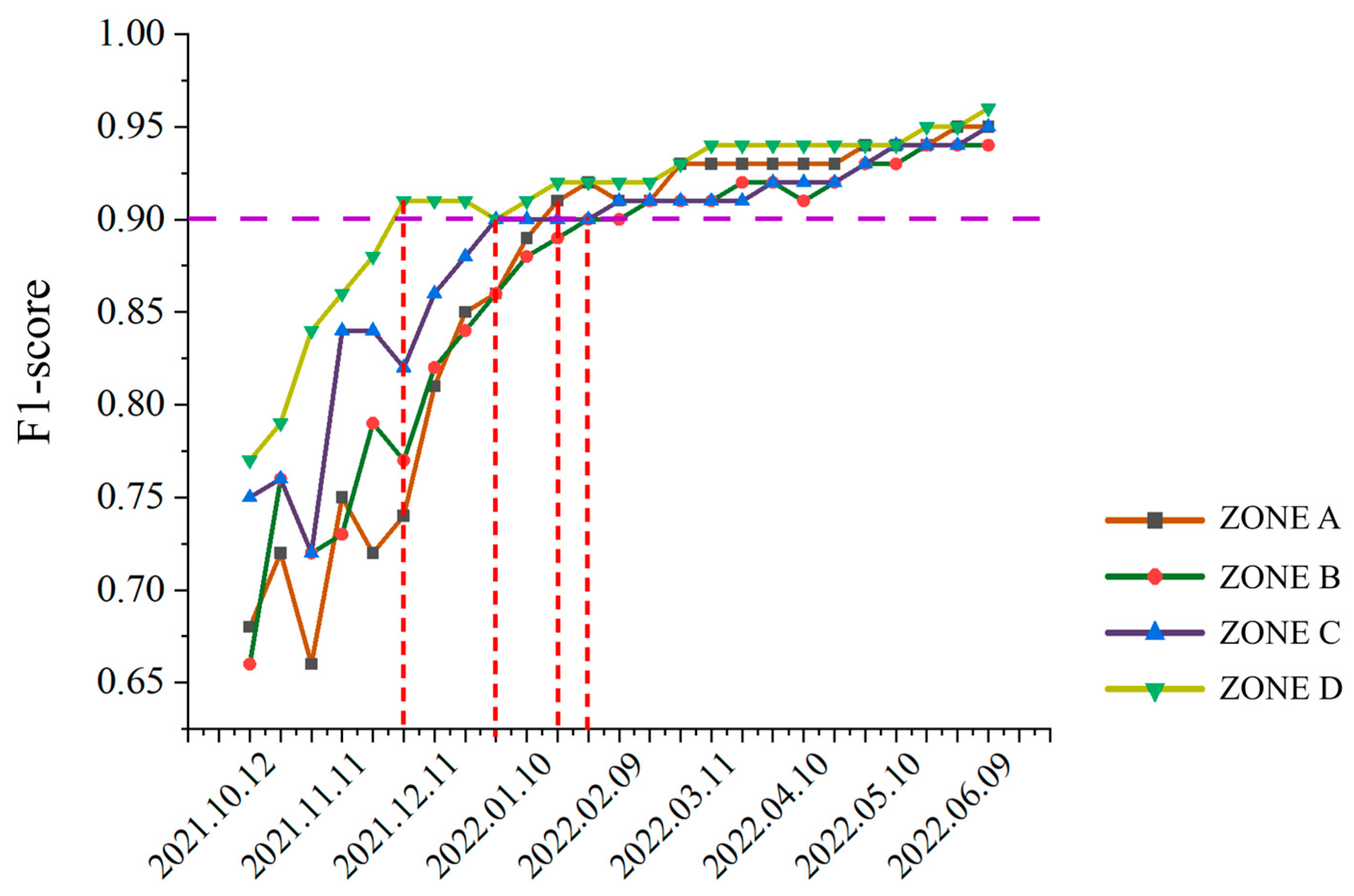
The criterion for the earliest identification time was set as the first time point at which the F₁ score for winter wheat classification exceeded 0.9. Based on the preceding experiments, the maximum F₁ score achieved in Zone A and Zone C was 0.95, while the remaining two zones reached 0.94 and 0.96, respectively. Therefore, an F₁ score threshold of 0.9 was adopted as the criterion for determining the earliest identification time.

The earliest identification dates were derived from the temporal trends shown in Figure 6. The results indicated that the earliest identification time for winter wheat was 1 December in Zone D, 31 December in Zone C, 2 January in Zone A, and 30 January in Zone B, corresponding to the first occurrence of an F₁ score exceeding 0.9. These findings highlight the spatial variability in phenological development across zones and validate the effectiveness of the proposed zone-specific classification strategy for achieving timely and accurate winter wheat identification.

4.3.3. Comparison Between Zonal and Non-Zonal Mapping Approaches

In this study, early-season winter wheat mapping results derived from the proposed zonal strategy were systematically compared with those obtained using a non-zonal approach in Shandong Province (

Table 6. Comparison of accuracy between non-zonal and zonal early mapping.

	Non-Zonal			Zonal
	Winter Wheat	Non-Winter Wheat	PA (%)	Winter Wheat	Non-Winter Wheat	PA (%)
Winter wheat	330	29	97.06	342	17	95.26
Non-winter wheat	10	538	94.90	5	563	99.12
UA (%)	91.91	98.18		98.56	97.07
OA (%)	94.03			97.63

and Figure 7). The results indicated that the zonal classification strategy significantly increased OA and improved the spatial consistency of the classification outcomes.

In terms of classification accuracy, the non-zonal method achieved an OA of 94.03%. In contrast, the zonal method yielded a markedly improved OA of 97.63%, with higher accuracies observed across all zones. Specifically, Zone C, where the planting area of winter wheat was extensive and winter crop types were relatively homogeneous, attained the highest OA of 98.94%. In Zone A, although the OA was comparatively lower at 95.76%, it still outperformed the non-zonal approach. The detailed accuracy assessments conducted for each zone provided additional evidence supporting the robustness and effectiveness of the proposed method: in Zone A (20 January), the UA and PA for winter wheat were 93.44% and 97.44%, respectively; in Zone B (30 January), these values reached 95.73% and 99.09%; in Zone C (31 December), they were 97.65% and 99.49%; and in Zone D (1 December), the PA reached 99.32%, with an OA of 97.02%.

Regarding identification timeliness, the non-zonal method typically recognizes winter wheat around mid-January. However, the zonal method allowed for earlier and zone-specific identification, which better aligned with local phenological development. Although Shandong Province lies entirely within the warm temperate zone, intra-provincial climatic variability—driven by topography and maritime influence—led to significant differences in the greening periods of winter wheat. For instance, in Zone D, located in the southwestern and northwestern inland zones (e.g., Heze and Liaocheng), winter wheat was sown earlier, and the greening stage was reached as early as 1 December. In contrast, the eastern coastal zones, such as Zone A (e.g., Qingdao and Yantai), experienced slower warming due to maritime regulation, and early identification was only feasible by 20 January. These findings demonstrated that the zonal strategy effectively accommodated zonal phenological variability, thereby improving both the accuracy and timeliness of early-season winter wheat identification.

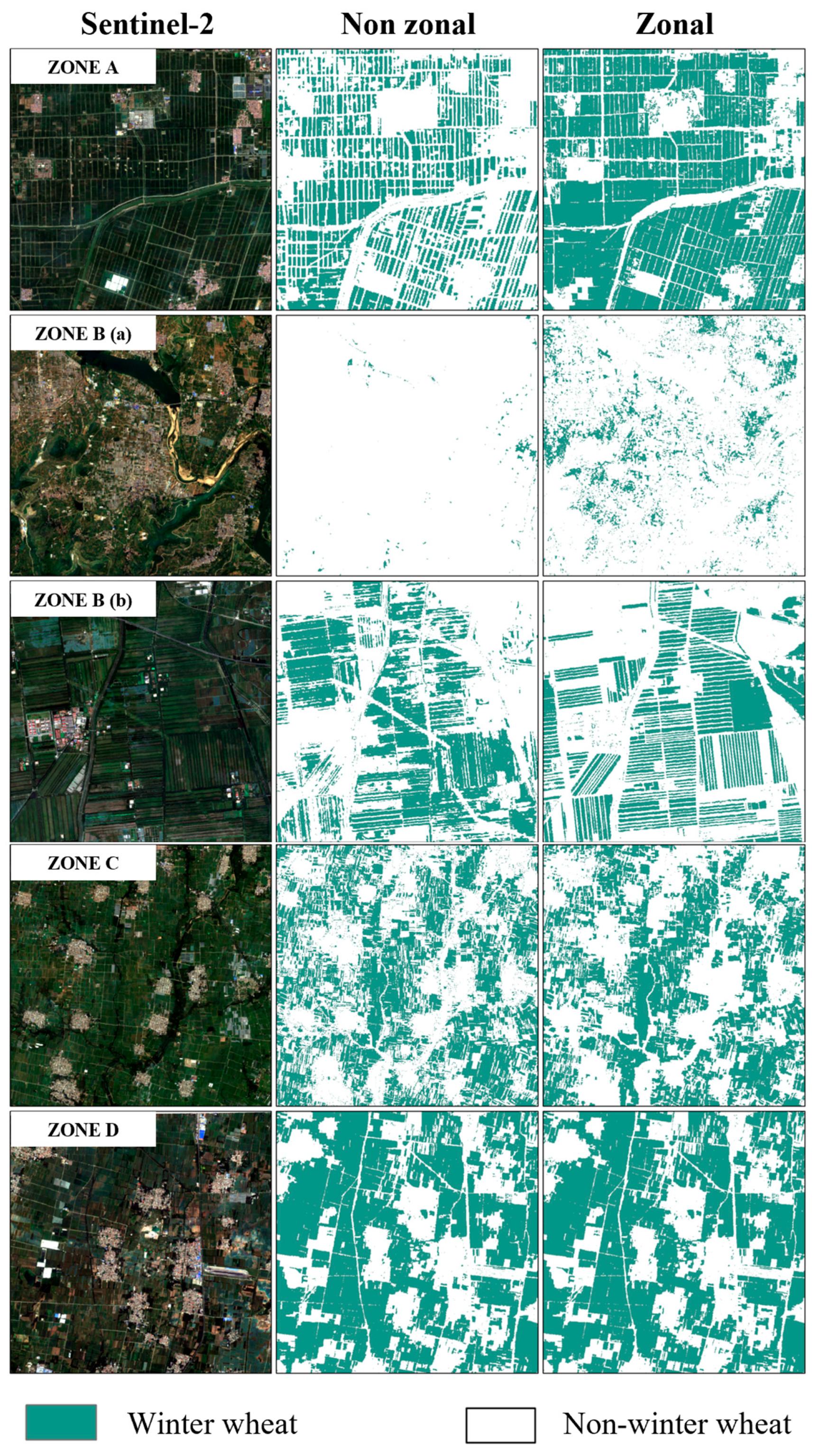
Figure 8 presents a detailed comparison of identification results across different zones. In Zone B(a), characterized by complex mountainous terrain, the non-zonal method exhibited substantial sparsity and failed to accurately delineate the spatial distribution of winter wheat. By contrast, the zonal approach successfully incorporated spatial heterogeneity across zones, thereby substantially enhancing classification performance.

In the flat terrain of Zone B(b), the zonal method successfully corrected the misclassification issues observed in the global results. It not only enhanced the detection accuracy of winter wheat but also significantly suppressed salt-and-pepper noise, thereby improving the overall classification performance. In Zones A and C, the zonal method also demonstrated notable improvements in both classification accuracy and consistency compared with the non-zonal approach. By contrast, the performance gap in Zone D between the two methods was less pronounced, likely due to the similar early identification times under both strategies in this zone.

4.3.4. Comparison with Official Statistics

To further evaluate the reliability of the classification results, the early-season winter wheat area in Shandong Province was quantitatively estimated and compared with official planting area statistics from the Shandong Provincial Bureau of Statistics (2021). The relative error was −3.6%, indicating that the identified area was slightly smaller than the reported figure, thereby demonstrating a high level of classification accuracy.

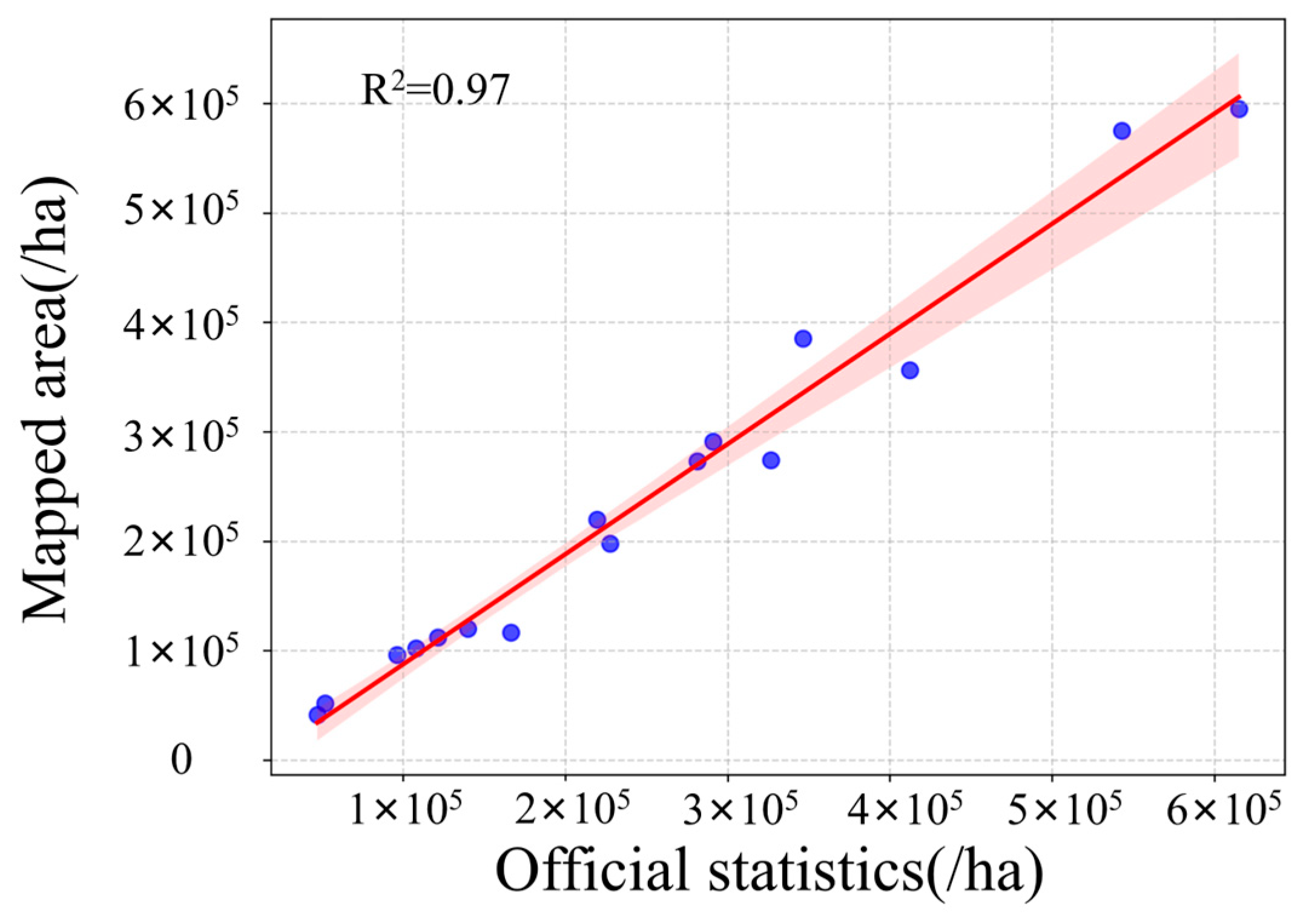
Moreover, to assess the spatial consistency of winter wheat classification, official statistics on planting areas from 16 prefecture-level cities in Shandong Province were gathered, and the mapped results were evaluated at the municipal level. The validation results (Figure 9) revealed a strong agreement between the zonal early-season identification results and the official statistics, with an R² value of 0.97. This further confirmed the reliability and robustness of the zonal classification approach proposed in this study.

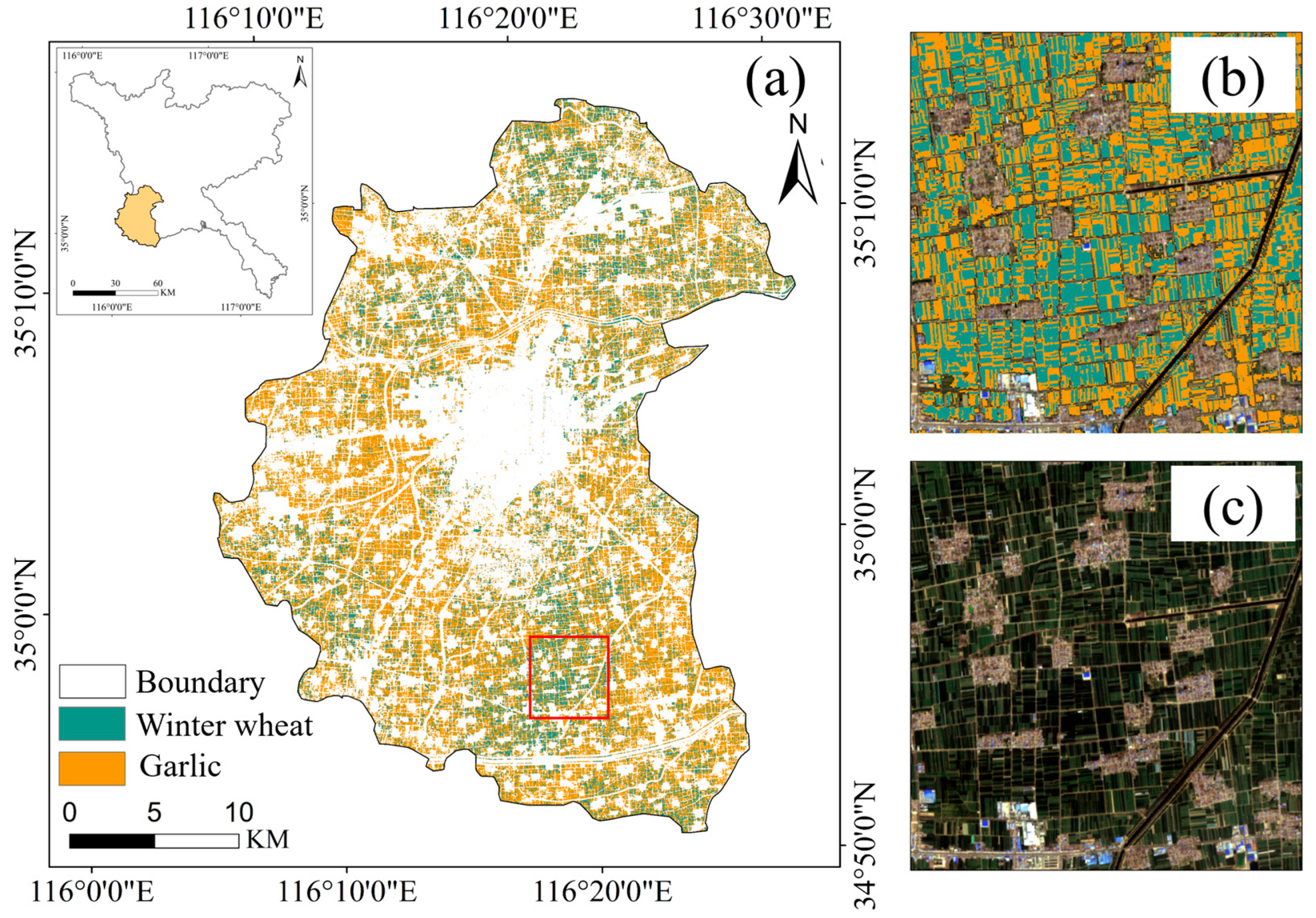
4.4. Confusion Analysis Between Winter Wheat and Garlic

In Shandong Province, garlic is one of the primary confounding overwintering crops besides winter wheat, due to its high similarity in both phenological cycles and spectral characteristics. This issue was particularly prominent in key garlic cultivation zones, such as Jinxiang County in Jining City, where adjacent and interspersed fields posed challenges for accurate classification.

To evaluate the feasibility of distinguishing garlic from winter wheat in remote sensing, this study selected Jinxiang County as a representative area. Multi-temporal remote sensing images from the 2021–2022 growing period were used to construct time-series features, and a total of 291 manually labeled garlic samples were obtained. Feature selection and classification experiments were subsequently conducted. The feature selection process identified that the top six features were VH, NDVI, IRECI, GCVI, RE2, and RED, three of which were also identified as key features in winter wheat classification within the same zone. This finding indicated that the proposed method exhibited a degree of feature universality when distinguishing crops with similar phenology and spectral responses.

Using the optimized time-series features for classification, an OA of 0.97 and an F₁ score of 0.94 were achieved, demonstrating that garlic and winter wheat remained distinguishable despite the close timing and similarity in feature expression. Recent studies have investigated the spatial mapping of winter wheat and garlic [5,13]. In this study, the proposed method achieved high classification accuracy, demonstrating its effectiveness in distinguishing between these spectrally and phenologically similar crops.

Additionally, distribution maps for winter wheat and garlic were generated to visually illustrate their spatial distribution characteristics in Jinxiang County (Figure 10a), along with classification results (Figure 10b) and detailed comparisons between imagery (Figure 10c). The results indicated that the garlic planting area was significantly larger than that of winter wheat. Moreover, the classification method using optimized features yielded high accuracy even in cases of adjacent planting of winter wheat and garlic.

5. Discussion

5.1. Cross-Year Experimental Result Validation

To further examine the effectiveness of the adopted strategy, an early-season winter wheat identification experiment was carried out using historical data from Liaocheng City, a representative area located within Zone C. Liaocheng was selected for this interannual transfer experiment due to its stable winter wheat cultivation regime and typical agroecological conditions, making it an ideal case for evaluating the generalizability and robustness of the proposed method across different years. For the 2017–2018 growing period. When the time-series remote sensing data were extended to 10 January 2018, the classification results achieved a stable F₁ score and an overall accuracy of 0.98, indicating high classification performance even under historical conditions. Figure 11 illustrates the early-season winter wheat mapping results for Liaocheng, along with comparative visualizations of the imagery and classification outcomes for selected zones.

In addition, the phenological stages of winter wheat in Liaocheng during the 2017–2018 and 2021–2022 growing seasons were compared using the NDVI peak detection method [41]. Results indicated that the sowing date in 2017 was 22 October, with the earliest identification time on 10 January; for 2021, the sowing date was 16 October, with the earliest identification achieved by 31 December. In both cases, winter wheat was successfully identified within approximately three months of sowing. These findings were consistent with existing studies in terms of both timing and spatial distribution patterns [17]. This result validated the coordination between the recognition timing of the proposed zonal method and the phenological characteristics of the crop, further supporting its temporal robustness and adaptability.

5.2. Comparison with Publicly Available Winter Wheat Datasets

This study employed publicly available winter wheat datasets for comparative analysis, including the 2021 winter wheat distribution map derived from the Automatic Training Data Generation (ATDG) framework, ChinaWheat10, and the 2021 winter wheat planting distribution map covering eight major producing provinces, ChinaWheatMap10. These publicly available datasets were developed at large spatial scales using uniform classification models, a strategy commonly adopted in previous studies [20,42]. However, such an approach often fails to fully account for the detailed differences across zones.

As illustrated in Figure 12, the proposed zonal classification strategy exhibited clear advantages in enhancing the separability between winter wheat and other land cover types. It also achieved superior delineation of field boundaries, with higher spatial clarity and classification accuracy. For instance, in Qingzhou City within Zone B—an area characterized by dense distributions of vegetable greenhouses and fragmented, irregular-shaped plots—the zonal strategy improved winter wheat identification performance by mitigating classification confusion.

In Zoucheng City within Zone C, which features hilly terrain and dispersed farmland with small field sizes, winter wheat mapping remained challenging. However, the zonal classification approach effectively improved classification outcomes under such complex zonal conditions, thereby enhancing the spatial mapping accuracy of winter wheat in mountainous zones.

5.3. Significance, Limitations, and Future Prospects

This study proposed a zonal early-season winter wheat identification framework that integrates phenological and environmental factors. Results demonstrated that by dividing Shandong Province into four zones and optimizing zone-specific classification strategies, high winter wheat early-season classification accuracy could be achieved. For Zone D in southwestern Shandong, characterized by flat terrain and higher average temperatures compared to other areas, winter wheat could be mapped as early as December, with an OA of up to 97.02%. In contrast, in Zone B, which is characterized by predominantly mountainous and hilly terrain with lower average temperatures, winter wheat could be identified as early as late January, achieving an OA of 97.52%. These findings validated the effectiveness of incorporating phenological and environmental heterogeneity into classification strategies, and also demonstrated the significant implications of the proposed framework for enhancing the timeliness and precision of early-season crop mapping. The proposed approach not only improves early-season crop mapping accuracy but also provides robust technical support for precision agriculture, food security monitoring, and disaster response efforts.

Despite these advancements, several limitations still remain in this study. With respect to remote sensing imagery, this study primarily relied on Sentinel-2 data with a spatial resolution of 10 m. However, from other early-season winter wheat mapping studies [43], the images with 10 m resolution had shown limitations in capturing field boundaries accurately in heterogeneous or mountainous regions. Existing research has investigated the impact of various remote sensing images on early-season crop classification [44,45]. Future work may benefit from the integration of multi-source satellite imagery with higher spatial resolution, such as GF-2 and Planet satellites, to extract finer spatial and temporal features and support more accurate early-season crop identification.

Regarding the zonal strategy, administrative counties were used as basic analytical units in the study due to the accessibility of statistical data and relevance to policy applications. Nevertheless, administrative divisions may not align with ecological patterns and often fail to capture spatial heterogeneity in key environmental variables such as climate, elevation, and soil properties, thereby constraining model generalizability. Recent studies have proposed regular grid-based or agroecological zoning schemes as alternatives to better reflect underlying environmental variability, offering promising directions for refining the current framework [46].

In this study, to generate different zones, we adopted a combination of the Silhouette Coefficient and the Elbow Method, along with the K-means clustering algorithm, which are widely used in the existing literature [25] and have been proven effective in delineating spatially homogeneous zones in our study. However, the choice of clustering metrics and algorithms can significantly affect the outcomes of zonal division. Therefore, future research will systematically compare various clustering strategies, such as hierarchical clustering and density-based clustering, and explore alternative clustering evaluation indices. These efforts aim to enhance the robustness and adaptability of the zoning framework under diverse topographic and phenological conditions.

Regarding the classification algorithm, this study exclusively employed the RF classifier, which has been widely validated in crop mapping for its robustness and interpretability [12,40]. While the method has demonstrated strong performance, we acknowledge the potential of alternative approaches. In future work, we plan to incorporate and compare additional algorithms, such as support vector machines, gradient boosting, and deep learning models, to further enhance classification accuracy and improve adaptability across diverse agricultural scenarios.

6. Conclusions

This study proposed a zonal early-season identification strategy to address the spatial heterogeneity in large-scale winter wheat mapping. By integrating phenological and environmental factors, Shandong Province was divided into four representative zones, each with tailored classification schemes. The results demonstrated significant improvements in accuracy, timeliness, and spatial consistency.

The main contributions are as follows:

(1) Zonal strategy effectiveness: Zoning based on phenological and environmental factors reduced large-scale heterogeneity and supported high classification accuracy.

(2) Optimized identification timing: Zone-specific identification windows were established. The earliest mapping occurred in Zone D in early December, with an OA of 97.02%. Zones A-C reached their optimal identification periods between late December and January, each attaining an OA above 95%.

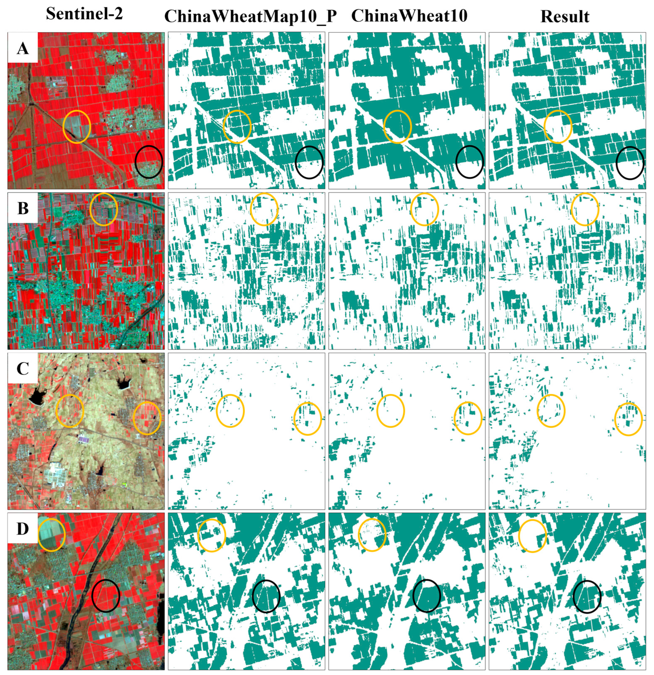
(3) Reliability and comparison: Validation against official statistics showed a relative area error of –3.6% at the provincial level and an R² of 0.97 across 16 municipalities. The zonal strategy improved overall accuracy by 3.6% over a non-zonal approach and outperformed public datasets such as ChinaWheat10 in spatial detail and classification precision.

(4) Feature adaptability: Zone-specific features enhanced classification. The method also successfully distinguished winter wheat from garlic, a spectrally similar crop, achieving an F₁ score of 0.94, indicating strong generalization capability.

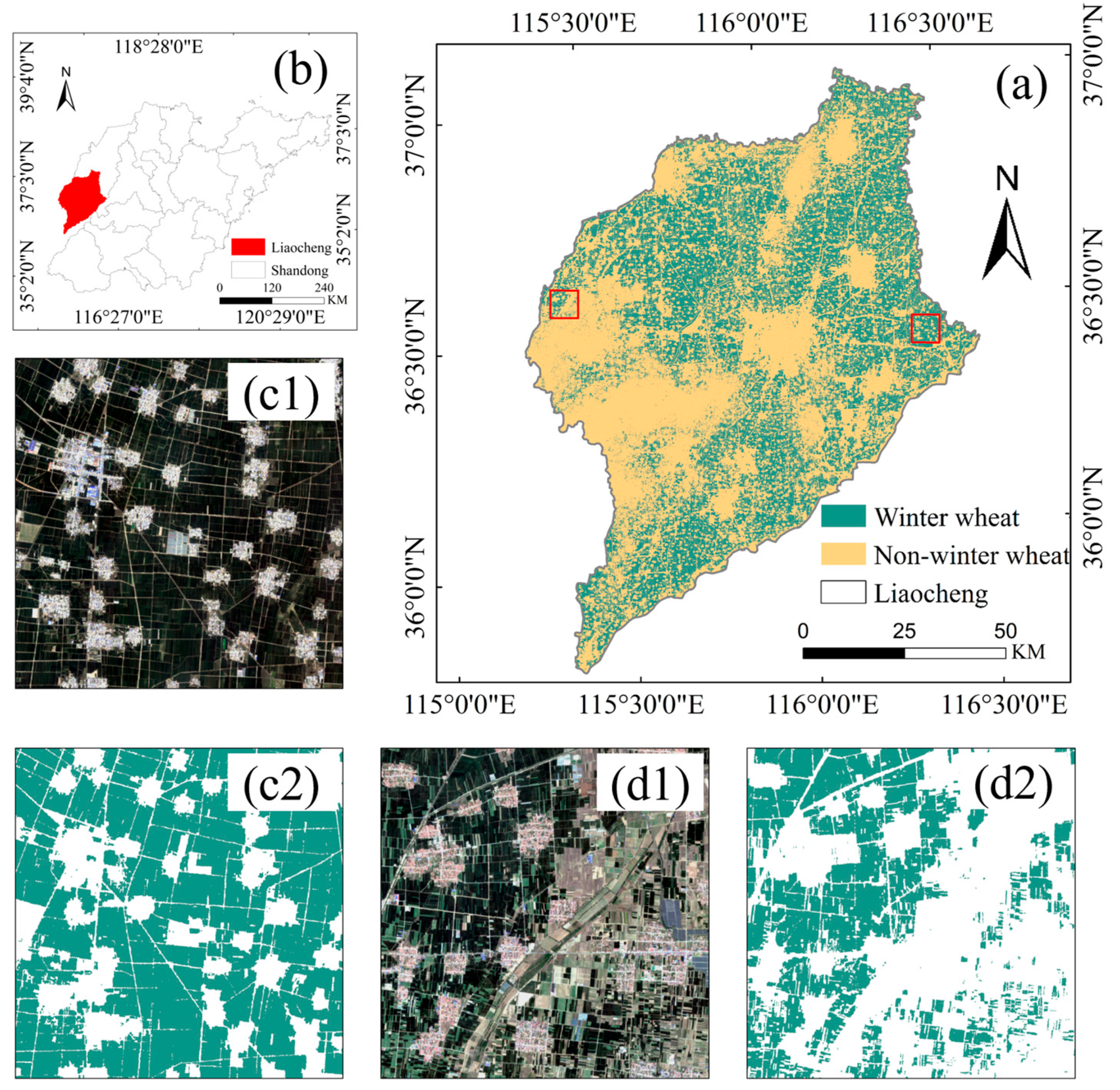
(5) Temporal robustness: Historical validation using 2017–2018 data in Liaocheng produced consistent results, with an OA of 98% and an F₁ score of 0.96. The identification timing matches historical phenology.

In summary, the proposed zonal strategy proved accurate, robust, and adaptable for early-season winter wheat mapping at large zonal scales.