Abstract
Locusts have always been among the important hazards affecting crop growth and the grassland ecological environment. Accurate and timely detection of locusts is crucial for effective control of insect development. Aiming at the problem of false detection and missed detection caused by locust occlusion and background similarity in complex field environments, this paper proposes a lightweight Attention-based Target Detection (ATD) model while constructing the dataset Real-Locust with the theme of Locusta migratoria ssp. manilensis. By introducing to attention mechanism and lightweight design, the model achieves a mean average precision (mAP) of 90.9% on the Real-Locust dataset, and the precision and recall rate are increased by 0.6% and 4.3%, respectively. At the same time, the number of parameters and computational complexity are reduced by 27.4% and 22.9%, showing that this provides an efficient solution for real-time monitoring of locusts.
1. Introduction
Locusts are one of the important causes of economic losses in global agriculture and grassland animal husbandry [1]. Locust plagues, floods, and droughts are called the three major natural disasters. In China, more than two million hectares of agricultural land are affected by locust invasion every year, which is of great harm to crops and food security [2]. Therefore, the establishment of an efficient, accurate, and intelligent pest monitoring and early warning system has become the key to improving disaster response capabilities [3].
Traditional locust monitoring methods mainly rely on artificial ground surveys, including the gradual investigation of locust eggs, nymphs, and adults [4]. These methods are usually implemented by local plant protection stations or professional organizations, but there are problems such as consuming a lot of manpower, material, and financial resources, low investigation efficiency, and difficulty in covering complex terrain areas such as lakes and swamps [5]. To improve monitoring efficiency, some studies have tried to introduce climate prediction [6], phenological prediction [7], and remote-sensing technology [8] to realize the dynamic analysis of pest situations at the regional level. However, in these technologies, climate prediction has a low spatial resolution due to its dependence on macro data, and phenological prediction lacks a consideration of small-scale spatial heterogeneity. These do not integrate high-resolution spatial data and landscape features, resulting in inaccurate spatial positioning of locust occurrence areas. Although remote-sensing monitoring has the advantages of real-time and wide-area coverage, it is difficult to realize the accurate identification of locust individuals due to the limitation of image resolution.
In recent years, great progress has been made in the combination of locust monitoring technology based on machine learning and remote-sensing technology. Tabar et al. [9] developed a model, PLAN, based on spatio-temporal deep learning, which uses crowdfunding data and environmental data to predict the migration pattern of locusts in East Africa. Experiments show that its AUC score reaches 0.9, which is significantly better than the traditional machine learning model. Kimathi et al. [10] used the MaxEnt niche model, combined with environmental variables such as temperature, precipitation, soil moisture, and sand content, to predict the breeding sites of desert locusts in East Africa. Shao et al. [11] monitored and predicted the severity of locust outbreaks in the Asian–African desert by combining MODIS time-series data and the Hidden Markov Model (HMM), and quantitatively evaluated the impact of locust outbreaks on crops using hyperspectral images. Gómez et al. [8] used near-real-time soil moisture data from the SMOS satellite and six machine learning algorithms to predict the breeding grounds of desert locusts and found that soil moisture data can provide sufficient prediction information 95 to 12 days before the locust appears. Sun et al. [12] proposed a dynamic prediction model based on support vector machine and multivariate time-delay sliding window technology. Combined with multi-source remote-sensing data and historical locust survey data, the dynamic prediction of desert locust swarms was realized 16 days in advance. Guo et al. [13] used support vector machine (SVM), random forest (RF), and maximum likelihood (ML) methods to study the formation mechanism of high-density patches of Asian migratory locusts based on time-series remote-sensing images. However, the traditional machine learning algorithm has a poor feature extraction ability in complex scenes, so it is difficult to meet the needs of high-precision locust detection.
Deep learning can automatically capture complex features in data through layer-by-layer feature extraction and generation mechanisms. Compared with traditional machine learning, it has a higher precision and efficiency in recognition tasks [14]. Ye et al. [5] developed the ResNet-Locust-BN model by improving the ResNet structure. Based on the training of RGB image samples in the field, the automatic identification of the species and instars of migratory locusts in East Asia was realized. The precision levels when distinguishing migratory locusts from rice locusts and cotton locusts were 93.60% and 97.80%, respectively, and the overall precision was 90.16%. Bai et al. [15] proposed a video target detection method for migratory locusts in East Asia based on the MOG2-YOLOv4 network. By combining background separation and deep learning technology, the problems of occlusion and blurring were solved. Experiments show that the average precision of the model is 82.33%. Aiming at the segmentation problem of camouflage locusts, Liu et al. [16] proposed an EG-PraNet model based on improving PraNet. By introducing a grouping reverse module and image enhancement technology, the segmentation precision was significantly improved, and the Dice and IoU indices were increased by 17.8% and 25.7%, respectively. At present, there are few studies on locust detection based on deep learning. The existing research mainly focuses on improving detection precision and efficiency, and the optimization of real-time and generalization ability still needs to be further explored.
As a lightweight and efficient target detection algorithm, YOLO (You Only Look Once) has been widely used in plant pest detection [17]. For example, to balance computational efficiency and detection performance, Li et al. [18] achieved 94.3% detection precision and 93.5% mAP in complex field environments by integrating cross-stage feature fusion (Hor-BNFA), spatial depth conversion convolution (SPDConv), and group shuffle convolution (GsConv). The model size is only 7.9 MB, which is better than the existing models. Liu et al. [19] aimed at solving the problem that the existing models usually find it difficult to capture the long-distance dependencies and fine-grained features in the image, resulting in a poor recognition effect in the case of a complex background. By integrating the hybrid convolution Mamba module in the neck network, introducing the similarity-based attention mechanism, and using the weighted bidirectional feature pyramid network, the disease recognition ability of the model in a complex background is significantly improved. The F1-score and mAP are 3.0–4.8% higher than YOLOv8, respectively. Zhang et al. [20] constructed a lightweight pest detection model, AgriPest-YOLO, based on YOLOv5. AgriPest-YOLO solves the problems of scale change and a complex background in light trap images by coordination and a local attention mechanism, grouping spatial pyramid pooling, and soft-NMS optimization. Zhu et al. [21] proposed an improved CBF-YOLO network based on YOLOv7, which achieved high-precision detection of damaged leaves of soybean pests by combining CSE-ELAN, Bi-PAN, and FFE modules. The mAP of the public dataset was 86.9%, and the mAP of the actual scene was 81.6%, which was still affected by light conditions, background complexity, and similarity of pest characteristics. Wang et al. [22] developed the Insect-YOLO model based on YOLOv8 and the CBAM attention module for the detection and counting of low-resolution farmland pest images and integrated the algorithm into the remote pest monitoring and analysis system. The mAP@50 of 93.8% was achieved on 2058 low-resolution images, which was superior to other baseline models.
At present, the research on locust detection based on deep learning is limited, and most of the existing methods focus on the target image with a single background, ignoring the challenges brought by the real field environment to the detection task. The precision and generalization performance in dealing with changing environments (such as illumination changes and target occlusion) must be improved [5]. In addition, existing models usually have a high number of parameters and computational complexity, which affect their deployment on resource-constrained mobile or embedded platforms [23]. To address these challenges, this study aims to develop a lightweight, efficient, and high-precision detection model for Locusta migratoria ssp. manilensis in complex environments. We will first construct a new dataset named Real-Locust, which includes locust images captured against diverse backgrounds, at varying densities, and in different poses. Then, we will propose an improved YOLOv8n-based model, called ATD-YOLO, which integrates modules such as AIFI, CBAM, and LTSC to enhance feature extraction capabilities and reduce model complexity. In the experimental phase, we will conduct extensive cross-validation and ablation studies to evaluate the effectiveness and efficiency of the proposed model. We will also compare it with other state-of-the-art models to demonstrate its advantages and provide a reliable solution for real-time monitoring of locusts in agricultural fields.
2. Materials and Methods
2.1. Dataset
2.1.1. Data Acquisition
This study uses Locusta migratoria ssp. manilensis images as a case study for model evaluation. Due to the problems of a single background and obvious features in the existing public datasets, it is difficult to meet the detection requirements in real scenes. Therefore, this study constructed a Locusta migratoria ssp. manilensis-themed dataset, Real-Locust, and the dataset samples are shown in Figure 1. Dataset construction mainly considers three aspects: real and complex background, changes in locust density, and diversity of poses. The data collection time is April 2024, and the weather is not deliberately selected to obtain images under different illuminations and morphologies, to improve the generalization ability of the model in different scenarios. The acquisition equipment is a DJI Mavic Mini UAV, equipped with an RGB camera. The image sensor is 1/2.3-inch CMOS, the effective pixels total 12 million, the equivalent focal length is 24 mm, the resolution of the captured image is 4000 × 2250 pixels, the aspect ratio is 16:9, and the camera resolution is 2720 × 1530. The height of the drone is less than 0.5 m and the angle of the pan-tilt camera is 90°. The acquisition method is to record and take indirect photos in a manually controlled, stationary flight mode. The video frame extraction technology is used to save each frame as a JPG image.
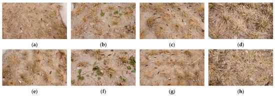
Figure 1.
Image samples in Real-Locust. (a–h) Dataset of images taken against different backgrounds and with different densities.
2.1.2. Dataset Creation and Preprocessing
To ensure the diversity and quality of the dataset, invalid images, such as heavily blurred and repeated images, were screened out. Finally, 304 locust images in the complex environment were obtained from the collected videos and pictures. The Labelimg (version 1.8.6) tool was used to label and generate TXT files corresponding to the pictures [24]. The files contain target categories and location information. The dataset is divided according to different acquisition times and acquisition areas, and the locust dataset is divided into a training set, verification set, and test set according to the ratio of 7:2:1 [25].
To further increase the robustness and generalization ability of the dataset, this study introduces a data enhancement method after dividing the dataset [26], which ensures the objectivity of the experimental results. Data enhancement methods include adding noise, adjusting brightness, random occlusion, rotation, cropping, translation, and mirroring. Each image is randomly selected in five ways to enhance it, and multiple enhancement operations may be superimposed on the same image according to a random probability. The enhanced image samples are shown in Figure 2. The training set is expanded to 1070, the validation set is expanded to 300, and the test set is expanded to 150. During the training process, YOLOv8 combines Mosaic data enhancement technology to further improve the performance of the model.
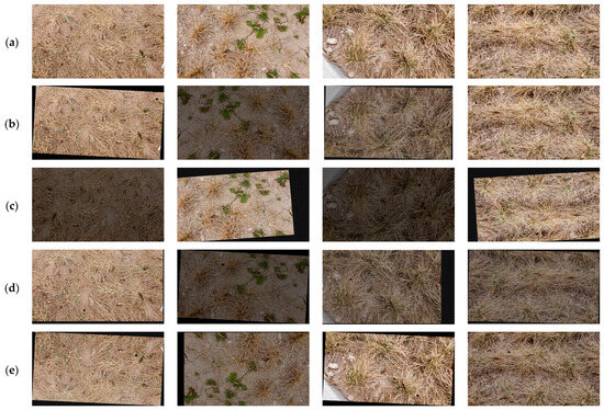
Figure 2.
Image enhancement. (a) Original image samples. (b–e) Enhanced image samples.
2.2. ATD-YOLO Model
The basic network used in this paper is the YOLOv8 network [27], which is a real-time object detection algorithm released by the Ultralytics development team on 10 January 2023. Compared with YOLOv5, YOLOv8 has been further improved in precision and speed, and its excellent performance makes it widely used in visual tasks such as target detection and instance segmentation.
The YOLOv8 model consists of three core components: Backbone, Neck, and Head. Among them, Backbone is responsible for basic feature extraction, which is mainly composed of Conv, C2f, and SPPF modules. The Conv module realizes efficient feature extraction of the input image through the Conv2d convolution layer, batch normalization, and SiLU activation function. The C2f module adopts the gradient shunt connection method to enhance the information flow richness of the network and further improve the feature expression ability. The SPPF module realizes robust processing of multi-scale inputs through three maximum pooling layers of different sizes. The Neck part adopts the combination structure of the feature pyramid network (FPN) and path aggregation network (PAN). Through top-down and bottom-up bidirectional feature fusion, the feature maps of different stages are fully integrated, and the feature representation ability of the model is significantly enhanced. The Head part introduces a new Decoupled Head design, which separates the classification and regression tasks into independent branches, optimizes the loss calculation process, and improves the flexibility and performance of the model.
The YOLOv8 algorithm includes five variants of different parameter sizes, such as n, s, m, l, and x. Among them, YOLOv8n is the model with the least number of parameters and the lowest computational complexity. Considering the applicability of the final model deployment, this study developed a locust detection model based on ATD-YOLO with YOLOv8n as the basic network. The model structure is shown in Figure 3.
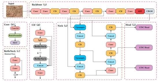
Figure 3.
(a) ATD-YOLO network structure; (b) Conv module structure; (c) BottleNeck module structure; (d) C2f module structure.
The ATD-YOLO model uses the AIFI module to replace the original SPPF module. By combining the two-dimensional sine–cosine position embedding and self-attention mechanism, the model’s ability to capture long-distance dependent information is enhanced. Location embedding assigns unique coding to each location to help the model understand the spatial structure, while the self-attention mechanism enhances the perception of the global context. It enables the model to accurately focus on the target features in the case of complex backgrounds and partial occlusion. The CBAM module introduces channel and spatial attention mechanisms to further optimize the expression of feature maps. The channel attention mechanism highlights important information by weighting the characteristics of each channel; the spatial attention mechanism focuses on the key areas in the image and enhances the extraction of local information. In addition, the LTSC module is used to replace the traditional detection head, and the lightweight shared convolution and separation batch normalization design is adopted to speed up the inference while maintaining the detection precision.
2.2.1. Attention-Based Intra-Scale Feature Interaction (AIFI)
The morphological characteristics of locusts are diverse and complex, including small shapes and low-contrast textures. In the YOLOv8 network, although the multi-scale pooling strategy is adopted to enhance the feature expression in the SPPF module at the end of the backbone network, its core mechanism still depends on the fixed-size pooling kernel. This fixed configuration limits the adaptability of the module to different-scale targets, especially when dealing with small targets, and the fixed-size pooling operation easily leads to the loss of feature details. To solve this problem, Zhao et al. [28] proposed an attention-based intra-scale feature interaction (AIFI) module, which combines position embedding and a multi-head attention mechanism to achieve adaptive feature enhancement. The proposed RT-DETR also shows that the deep feature S5 contains richer semantic information, while the shallow features S3 and S4 contain less semantic information. Only applying the encoder to S5 cannot only reduce the computational complexity but also maintain the detection performance.
The AIFI module is a visual feature enhancement module based on the Transformer architectural design, and its network structure is shown in Figure 4. The module uses a four-dimensional tensor [B, C, H, W] as the input feature map. Firstly, the spatial dimension is folded into a sequence dimension by a dimension transformation, and the feature map is reshaped into a serialized representation of [B, H × W, C]. In this process, the module synchronously generates a two-dimensional sine–cosine position code with spatial perception ability: by creating horizontal (grid_w) and vertical (grid_h) coordinate grids, the embedded dimension is split into four subspaces, and the sine and cosine components of different frequencies are calculated, respectively. Finally, a position coding matrix [1, H × W, C] with the same dimension as the feature sequence is formed. The coding regulates the frequency decay rate by the temperature parameter τ = 10,000.0 to ensure that different spatial locations have unique coding characteristics.
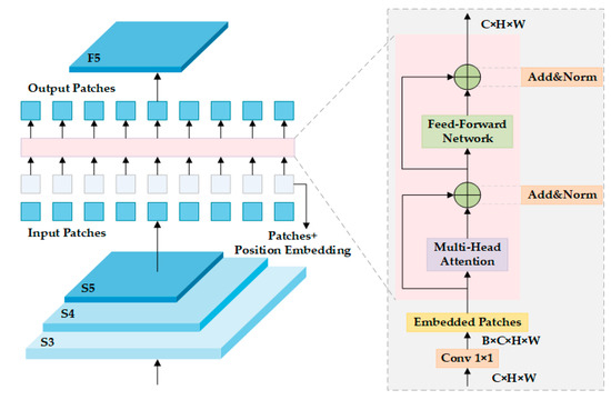
Figure 4.
AIFI logic structure.
Subsequently, the feature sequence is fused with the position coding and input into the Transformer coding layer. The coding layer consists of two core components: one is a parallel multi-head self-attention mechanism based on the num_heads configuration (as shown in Formula (1)) [29], which captures long-distance feature interaction by establishing global dependencies.
In the formula, Query (Q) represents the query correlation, Key (K) represents its characteristics, and Value (V) represents the query value. dK is the dimension of each attention head (as shown in Formula (2)), and the scaling factor is used to stabilize the gradient calculation. The mechanism calculates the attention weight by querying the (Q)-key (K) matching degree and then sums it with the value (V) to realize the feature interaction across spatial locations.
The other is that the feedforward network adopts an extended-compression structure (as shown in Formula (3)) [30]. The feature dimension is first extended to cm and then projected back to the original channel number C, and the nonlinear transformation is realized with the GELU activation function.
In the formula, extends the feature dimension to the middle dimension cm (usually cm > C), and (cm × C) compresses it back to the original channel number. The GELU activation function implements an adaptive gating mechanism through the cumulative distribution function of the standard normal distribution to enhance the nonlinear expression ability.
The whole process is stably trained by the regularization system (including dropout and layer normalization of a configurable order). The final feature sequence recovers the spatial dimension (as shown in Formula (4)) through the inverse transformation Reshape operation, and it outputs the [B, C, H, W] feature map with the same shape as the input. To further optimize feature extraction, a convolutional layer (Conv) is added before the AIFI module to capture local features. This combined architecture of ‘local convolution + global Transformer’ improves the detection precision of targets at different scales by complementing the local receptive field of the convolution kernel with the global interaction of self-attention.
2.2.2. Convolutional Block Attention Module (CBAM)
In the field of computer vision, the attention mechanism is the ability to imitate the selective focus of human vision. It prioritizes the visual information most related to the current task by dynamically adjusting the importance weight of each region of the input image [31]. The Convolution Block Attention Module (CBAM) [32] is a lightweight attention mechanism composed of channel attention (CA) and spatial attention (SA) in series, and its network structure is shown in Figure 5. The overall process is that the input features first refine the importance of the channel dimension through channel attention, then strengthen the spatial information of the key areas through spatial attention, and finally output the adjusted features.
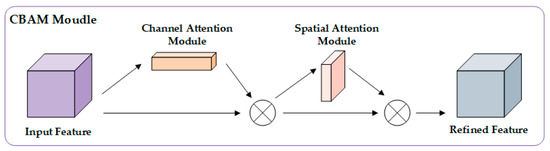
Figure 5.
CBAM logic structure.
The channel attention module structure is shown in Figure 6. The input feature map first extracts the statistical features of the channel through global average pooling and global maximum pooling. The dual pooling results are nonlinearly mapped by a shared multi-layer perceptron (MLP), where the MLP uses a reduced-dimensional design to reduce the number of parameters. After the output results of the two branches are added element by element, the channel weight matrix is generated by the Sigmoid function. The calculation process can be expressed as
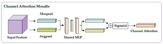
Figure 6.
Channel attention logic structure.
Among them, AvgPool and MaxPool, respectively, perform global average pooling and maximum pooling on the input feature graph X to generate two [B × C × 1 × 1] channel description vectors, as shown in Formulas (6) and (7). MLP is a multi-layer perceptron with shared weights, and the structure is C→C/r→C (r is the compression ratio, default 16). σ is a Sigmoid function, which generates a channel weight matrix . Finally, the input feature map is multiplied by the channel weight channel by channel, and the feature enhancement of the channel dimension is realized.
The spatial attention module is shown in Figure 7. The input feature map is averaged and max-pooled along the channel dimension to generate two single-channel spatial feature maps. After the two features are spliced along the channel dimension, the weight distribution of the spatial position is learned through a fixed-size convolution layer (such as a 7 × 7 convolution). The convolution results are activated by the Sigmoid function to generate a spatial weight matrix. The calculation process can be expressed as
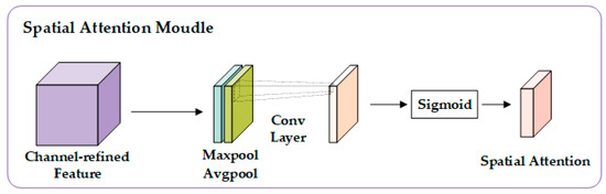
Figure 7.
Spatial attention logic structure.
Among them, the mean and maximum values of the channel attention output X′ along the channel dimension are calculated, respectively, and two [B × 1 × H × W] spatial feature maps are generated, as shown in Formulas (9) and (10). Feature splicing and convolution splice the two features into [B × 2 × H × W] along the channel dimension, fuse the spatial information through the convolution layer with the convolution kernel size of k × k (default 7 × 7), and output the single channel weight matrix. σ is the Sigmoid function, which generates the spatial weight . Finally, the channel attention output feature is multiplied by the spatial weight position by position to complete the feature calibration of the spatial dimension.
2.2.3. Lightweight Shared Convolution (LTSC)
For field locust detection, the size and inference speed of the model directly affect its deployment and application in the actual agricultural environment. In YOLOv8n, the number of parameters of the detection head accounts for 25.0% of the total, and the calculation cost is 36.4%. To further reduce the number and complexity of the model parameters and enhance its applicability to embedded devices, this study designs a new lightweight detection head structure, LTSC, to replace the original detection head.
Traditional object detection frameworks (such as YOLO series) usually design independent detection branches for feature maps of different scales, and each branch processes object detection tasks of corresponding scales through exclusive convolutional layers [33]. Although the framework can adapt to the change in target scale, it has some defects: the independence of parameters between branches leads to the redundancy of model parameters, and the independent training parameters of each branch are prone to cause multi-level feature coupling and increase the risk of overfitting. It is worth noting that the multi-scale feature layer essentially has similar spatial relationship modeling capabilities, which have been verified in detectors using parameter-sharing mechanisms such as RetinaNet and FCOS [34,35]. Based on that, this study proposes a lightweight shared convolution detection head structure, which realizes the efficient utilization of parameters through cross-level reuse of convolution kernels. The LTSC structure is shown in Figure 8 (the green module is an independent computing unit, and the orange part is a cross-layer shared component).
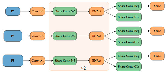
Figure 8.
LTSC logic structure.
However, simply sharing convolutional layers ignores the distribution differences of features at different levels. If the global batch normalization (BN) is directly applied to the shared convolutional layer, the mixed calculation of statistics (mean and variance) of different feature layers will introduce distribution bias. If group normalization (GN) is used, although this problem can be alleviated, it will increase the computational complexity of the inference phase. Inspired by the idea of hierarchical adaptive normalization in NAS-FPN, this study uses a separate normalization system to design an independent BN statistic calculation path for each feature level based on the shared convolution layer. This scheme not only retains the high efficiency of parameter sharing but also maintains the independence of feature distribution through hierarchical exclusive normalization operation, and finally realizes the dual optimization of computational efficiency and detection precision.
In the branch processing flow of LTSC, the multi-scale feature list from the Neck part first adjusts the number of channels through a 1 × 1 convolution and then passes through a double-layer 3 × 3 convolution module with shared parameters and an independent batch normalization (BN) layer. Through this combination of ‘shared convolution + independent BN’, not only is a lightweight parameter realized but also the normalized independence of different-scale features is retained. Finally, the features will return to the regression branch and the classification branch. The regression branch outputs the distribution parameters of the 4 × reg_max channel through a 1 × 1 convolution (reg_max is the number of discrete intervals) and adjusts the regression scale through the learnable Scale module. The regression coordinate is calculated by the distribution representation: for each bounding box coordinate (such as the center point x), the model predicts reg_max discrete probability values , and the final coordinate is obtained by the integral Formula (11):
The classification branch directly outputs the probability of n categories through a 1 × 1 convolution, and the classification score is activated by the Sigmoid function, as shown in Formula (12):
The output of the two branches is spliced in the channel dimension to form the final output of each detection layer. In the inference stage, the outputs of all scales are concatenated and decoded: the distribution parameters of the regression branch are converted into coordinate offsets through the Distribution Focal Loss (DFL) module, and the DFL optimizes the learning of the discrete distribution by focusing on loss, as shown in Formula (13).
In the formula, y is the continuous value of the true coordinates, and i and j are adjacent discrete intervals. Combined with the dynamically generated anchor points (calculated by make_anchors according to the size and step size of the feature map) and step size information, the actual bounding box coordinates are decoded by dist2bbox. The calculation process is shown in the following formula:
In the formula, is the center coordinate of the anchor point, is the predicted offset, and is the scale coefficient of the scale module learning. The output of the classification branch is activated by Sigmoid to obtain the category probability. The dynamic anchor mechanism automatically reconstructs the grid when the input size changes to ensure the adaptability of different-resolution inputs. The anchor point coordinates are generated as shown in Formula (18).
In the formula, (k, m) is the grid position of the feature map, and W and H are the width and height of the feature map.
3. Results
3.1. Experimental Environment and Parameter Settings
All experiments in this study were performed using Python 3.10 and PyTorch 2.1.0, and the training used an RTX A5000 GPU with 24 GB of memory. The specific experimental environment and parameter settings are shown in Table 1, and the key training parameter settings are shown in Table 2 to ensure the transparency and repeatability of the experiment.

Table 1.
Experimental environment and parameter settings.
Table 2.
Key parameter settings.
3.2. Model Evaluation Indicators
In this paper, precision, recall, F1-score, mAP, params, and GFLOPs are used as evaluation indices to measure the improvement effect. The precision P is the probability of the true positive sample in the sample that is predicted to be positive. The formula is
In the formula, denotes the number of positive samples correctly predicted, and denotes the number of negative samples incorrectly predicted as positive samples. The smaller the , the higher the precision, and the fewer the non-locust targets that are misjudged as locust targets.
The recall rate R is the probability that all the samples predicted to be positive are positive samples. The calculation formula is
In the formula, represents the number of positive samples that are wrongly predicted as negative samples. The smaller the , the higher the recall rate, and the fewer the locusts that are missed.
In some cases, there is a contradiction between precision and the recall rate, which requires comprehensive consideration. To this end, a comprehensive index F1-score that takes into account both is introduced. The calculation formula is
Here, is a minimal constant that prevents the denominator from being 0.
The average precision (mAP) of all classes is the mean of the detection precision of all classes. The calculation formula is
In the formula, c represents the total number of categories of target detection, and P (R) is a curve drawn with the recall rate as the X axis and the precision as the Y axis. The area enclosed by the curve and the coordinate axis is the average precision. In this paper, the model only needs to identify locust species targets, so the mAP value is the value.
The number of parameters is the total number of all trainable parameters in the model, which directly affects the model complexity, training time, and inference speed. The number of floating-point operations is the number of floating-point operations performed per second during model inference. The lower the number of parameters and floating-point operations, the lower the complexity of the algorithm, and the lighter the model.
In addition, the Mean Activation Value (MAV), Activation Entropy (AE), Background Mean Activation (BMA) and Activation Contrast (AC) were used as the analysis indexes of the heat map. Among them, the MAV reflects the intensity of the model’s attention to the target area, and the calculation formula is
In the formula, Ai is all the activation values in the target box, and N is the total number of pixels in the target box. The higher the value, the stronger the activation of the model to the target area, indicating that the area is the key area for model judgment.
AE is used to measure the concentration of activation values in the target area. The calculation formula is
In the formula, 1 × 10⁻⁸ is the minimum value, avoiding cases where the denominator is 0 or the logarithm is not defined, and N is the total number of pixels in the target box. The lower the entropy value, the more the model’s focus on the target is concentrated in a few key areas, and the feature discrimination is strong.
BMA reflects the ability of the model to suppress background noise. The calculation formula is
In the formula, Bj is the activation value of all non-target areas in the image, and M is the total number of pixels in the background area. The lower the value, the weaker the activation of the background region, the better the background suppression effect of the model, and the stronger the anti-interference ability.
AC is used to measure the activation difference between the target and the background. The calculation formula is
In the formula, 1 × 10⁻⁸ is the minimum value, avoiding a denominator of 0. The higher the value, the greater the difference between the activation of the target and the background, and the stronger the discrimination ability of the model to the target.
3.3. Cross-Validation Experiments
To evaluate the robustness and generalization ability of the model, this study employed five-fold cross-validation. Specifically, the training and validation sets were combined into a single dataset (a total of 1370 images), which was then divided into five subsets. In each experiment, four of these subsets were used as the training set, while the remaining one served as the validation set. This process was repeated five times to ensure that each subset participated in the validation phase. This approach helps minimize evaluation bias caused by uneven data partitioning, providing a more reliable assessment of the model’s performance.
In each fold of the experiment, the model underwent the standard training process and was then evaluated on the validation set. Performance metrics such as precision, recall, F1-score, and mean average precision (mAP) were recorded. After completing all the folds, the average values and standard deviations of these metrics were calculated to provide a more stable assessment of the model’s performance. The results of these experiments are shown in Table 3.
Table 3.
Results of the 5-fold cross-validation experiment.
As shown in Table 3, the model’s performance on the validation set was relatively consistent, with an mAP of 92.3% and a standard deviation of 0.9%, indicating minimal fluctuation across different folds and demonstrating good robustness. The standard deviations of precision (P) and recall (R) were 1.7% and 1.9%, respectively, while the F1-score had a standard deviation of only 0.3%, further confirming the model’s balance and consistency across folds. Based on the cross-validation results, the model with the highest mAP on the validation set was selected for the final evaluation on the test set. Table 4 presents the comparison of the selected best-performing model on the validation set with its results on the test set.
Table 4.
Comparison of the experimental results.
3.4. Ablation Experiment
To verify the effectiveness of the proposed improved model, this experiment used YOLOv8n as the basic model and used the self-made locust dataset, Real-Locust, and the same equipment to perform eight groups of ablation experiments on the improved methods proposed in Section 2.2.1, Section 2.2.2 and Section 2.2.3. To verify the stability of the model, each group of experiments was repeated five times, and the results were taken as the mean ± standard deviation. The model was evaluated using P, R, mAP@50, mAP@50:95, F1, Params, GFLOPs, and model size. The experimental results are shown in Table 5.
Table 5.
Ablation experimental results.
The ablation experiment results show that the original YOLOv8n model exhibits a certain basic performance in the target detection task, P = 0.900 ± 0.007, R = 0.820 ± 0.009, mAP@50 = 0.882 ± 0.005, and mAP@50:95 = 0.420 ± 0.010. However, it has problems with a high parameter quantity and computational complexity. The YOLOv8n + CBAM algorithm improves R by 0.85% and mAP@50:95 by 2.4% by introducing a channel-spatial attention mechanism, which significantly improves the detection performance of the model under different IoU thresholds. However, P decreased by 0.44% and F1 decreased by 0.81%, indicating that the attention mechanism may introduce feature redundancy while improving the positioning accuracy. Based on the AIFI module, YOLOv8n + AIFI significantly improves P by 1.22% and R by 1.46%, and the parameter amount is compressed by 7.18%, which verifies its ability to optimize feature extraction efficiency. However, GFLOPs decreased by only 3.6%, indicating that the module has a limited optimization of computational complexity and needs further improvement in combination with a lightweight design. YOLOv8n + LTSC achieves a parameter compression of 25.2% and GFLOP reduction of 21.7%, while R is increased by 2.56% through a lightweight shared convolution detection head. The results show that the separated normalization can effectively retain the target motion information while reducing redundant calculation, which is suitable for real-time detection scenarios. The combined scheme of YOLOv8n + AIFI + LTSC reduces the number of parameters by 27.5% and GFLOPs by 22.9%, while R increases by 3.78%, and the model size is the smallest, achieving a better balance between performance and a light weight. However, mAP@50:95 only increased by 0.71%, reflecting the influence of a lightweight design on a high IoU threshold detection ability. YOLOv8n + AIFI + CBAM combines the advantages of AIFI and CBAM. The algorithm P is increased by 1.22%, F1 is increased by 1.84%, and mAP@50:95 is optimal. Compared with YOLOv8n + AIFI, R is increased by 2.88% and mAP@50 is increased by 1.24%, which proves that the synergistic effect of the attention mechanism and feature interaction can effectively compensate for the information loss caused by a light weight. In the scheme of YOLOv8n + CBAM + LTSC, R increased by 2.07% while the parameter quantity was compressed by 23.1%, but mAP@50:95 decreased by 0.24% and F1 decreased by 0.09%. This indicates that the simple superposition of the attention mechanism and light weight may lead to a decrease in feature expression ability, and the module coupling method needs to be further optimized. ATD-YOLO achieves a 27.4% reduction in the number of parameters and a 22.9% reduction in GFLOPs by integrating the advantages of multiple modules. At the same time, R is increased by 5.49%, mAP@50 is 0.904 ± 0.012, and F1 is optimized to 0.886 ± 0.010. Although mAP@50:95 only increases by 1.67%, it achieves the optimal balance between GFLOPs and model size while maintaining high-precision detection through efficient feature interaction and modular compression, combined with an attention mechanism to compensate for lightweight information loss.
3.5. Performance Comparison with Baseline Models
To further verify the effectiveness of the improved network model in the complex environment locust detection task, under the same experimental equipment, experimental parameters, datasets, and training strategies, the experimental results of some better performance target detection models are compared with the experimental results of the improved network model in this paper, including YOLOv3-tiny, YOLOv5n, YOLOv6n, YOLOv8n, YOLOv9t, YOLOv10n, YOLOv11n, and YOLOv12n [36]. The evaluation index is the same as in Section 3.3. The experimental results are shown in Table 6.
Table 6.
Comparison of various detection models.
The experimental results show that the improved ATD-YOLO achieved a good performance on multiple performance indicators. P increased from 0.904 to 0.91, slightly higher than other models, which indicates that it is better at reducing error detection and can more accurately distinguish between the target and non-target. R increased by 4.3%, which is significantly better than other models, indicating that the model has made significant progress in reducing missed detection. The mAP@50 reached 0.909, which exceeded the other eight models and increased by 2.3% compared with the basic network YOLOv8n. The mAP@50:95 is increased from 0.424 to 0.431. Although it is slightly lower than YOLOv11n, it still exceeds the original YOLOv8n and other models, which indicates that the precision of target detection under different IOU thresholds is improved. In F1, the improved ATD-YOLO achieved a maximum value of 0.89, indicating that it achieved good results in balancing precision and recall. In terms of the number of parameters, complexity, and size of the model, although it is slightly lower than YOLOv9t, YOLOv11n, and YOLOv12n, it is greatly improved compared with other models. Overall, the improved ATD-YOLO does well at balancing the computational efficiency and detection performance.
In summary, the ATD-YOLO model proposed in this paper has certain advantages in accurately detecting locusts in complex agricultural environments.
3.5.1. Significance Analysis of ATD-YOLO, YOLOv8n, and YOLOv11n
In this experiment, YOLOv11 was added for comparison. Each group of experiments was repeated five times, and the results were taken as the mean ± standard deviation. Recall and mAP@50 were selected as evaluation indexes. Recall directly determines the missed rate of pest detection, which is the core index of agricultural application, while mAP@50 corresponds to the average accuracy of IoU = 0.5, which is more in line with the demand of “target roughly positioning can trigger prevention and control” in agricultural scenarios.
As shown in Figure 9, ATD-YOLO is significantly better than YOLOv8n and YOLOv11n in recall and mAP@50. In terms of recall, the mean value of ATD-YOLO (0.865) was 3.3% higher than that of YOLOv11n (0.837). There was no overlap in the box plot, and the t test showed a significant difference (p < 0.001). In terms of mAP@50, the mean value of ATD-YOLO (0.904) covered the upper limit of YOLOv11n performance, which was significantly increased by 0.9% (p < 0.05). Although YOLOv11n is slightly better at high IoU thresholds, ATD-YOLO has more of an advantage in striking an accuracy–efficiency balance through collaborative optimization of a light weight and attention mechanisms, providing a better solution for resource-constrained agricultural scenarios.
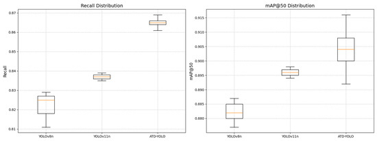
Figure 9.
The experimental results of different models are compared with the box plot.
3.5.2. Performance Comparison of ATD-YOLO, YOLOv8n, and YOLOv11n
Figure 10 shows the mAP@50 and total loss comparison curves of the improved models ATD-YOLO, YOLOv8n, and YOLOv11n.
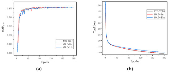
Figure 10.
The experimental results of different models are compared. (a) mAP@50 curve; (b) total loss graph.
In general, from the comparison of the mAP@50 curve, it can be seen that ATD-YOLO has a relatively high detection precision for the target at the initial stage of training, and the training process has no obvious fluctuation and is relatively stable. The initial convergence of YOLOv8n is slow, and there is an early stop phenomenon. Although YOLOv11n has a high precision in the later stage, it fluctuates frequently and plummets obviously, and there may be overfitting problems. In the comparison of the Total Loss curve, it can be seen that ATD-YOLO performs best. Although its initial loss value is slightly higher than YOLOv11n, the training process is more stable, the descent curve is smoother, and the final convergence effect is significant. Although YOLOv11n has a fast convergence speed in the early stage, there are slight fluctuations in the later stage, and there is still room for optimization. The comparison results further verify that the ATD-YOLO model has a better detection effect than other models.
3.6. Visual Analysis
To enrich the method of evaluating the performance of the ATD-YOLO algorithm, this section selects several models with better effects to conduct comparative experiments from two perspectives. First, the real locust test set is divided into three categories, and all models are verified by locusts with different density distributions. The classification details are shown in Table 7. Secondly, the gradient weighted class activation mapping [37] (Grad-CAM + +) method is used for visualization and analysis.
Table 7.
Locust density distribution rules.
3.6.1. Comparison of Test Results of Different Distribution Densities
To more intuitively illustrate the detection performance of the algorithm proposed in this paper, this section of the experiment selected three scenarios under different density conditions for display and compared those with the representative models (YOLOv8n and YOLOv11n). The detection results are shown in Table 8 and Figure 10.
Table 8.
The detection results of the model under different density conditions.
The table data show that YOLOv8n, YOLOv11n, and ATD-YOLO have the best performance in medium-density scenarios. R (0.913), mAP@50 (0.967), and F1 (0.932) of ATD-YOLO were all ahead, and P (0.957) of YOLOv11n was the highest. In the low density, ATD-YOLO had the best comprehensive performance (F1 = 0.858), and YOLOv11n had the lowest R-value (0.782). At the high density, the F1 (0.884) of ATD-YOLO and the R (0.86) of YOLOv11n were better, and the indicators of YOLOv8 n were generally lagging.
YOLOv8 has obvious shortcomings: In low-density scenarios, its mAP@50:95 is only 0.398, reflecting that the feature extraction module does not capture the locust target features, which may be more dispersed and relatively small at a low density, and it is difficult to accurately identify the target under stricter detection standards, resulting in a poor detection accuracy under complex evaluation indicators. In the high-density scene, the recall rate is reduced to 0.814, indicating that the detection head has insufficient instance segmentation and positioning capabilities in the overlapping area of the target when dealing with dense locust targets, resulting in missed detection. The defect of YOLOv11n is reflected in the fact that the recall rate is only 0.782 under low-density conditions, which is much lower than 0.896 at the medium density and 0.86 at the high density, indicating that its initial feature extraction layer is not sensitive enough to the sparse distribution of locust targets. For example, when the number of locusts is small and the distribution is sparse under a low density, the model struggles to quickly search for and locate the target, resulting in a high missed detection rate. The shortcomings of ATD-YOLO include, on the one hand, an mAP@50:95 of 0.377 in low-density scenarios, indicating that for small-sized locust targets that may exist at a low density, the down-sampling and up-sampling strategies of the feature extraction network fail to fully extract and recover small target features, resulting in a limited performance under high-precision detection standards.
It can be seen from Figure 11 that YOLOv8n and YOLOv11n still have some shortcomings in detail processing. For example, in the Level I scenario, they did not detect locusts in half of the body; in the Level II scene, there are many false detections and missed detections, and other objects are mistaken for locusts; in the Level III scenario, individual locusts are hidden in weeds and have a dense distribution in small areas, which increases the difficulty of detection, resulting in missed detection and repeated detection. ATD-YOLO shows certain advantages. When the target is densely distributed or occluded, it can identify the target more accurately and reduce the occurrence of missed detection.
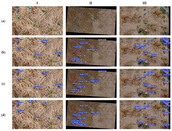
Figure 11.
The detection results of different model locusts under different density conditions. (a) Original GT image; (b) YOLOv8n test results; (c) YOLOv11n test results; (d) ATD-YOLO test results. The blue box indicates the detection result, the red box indicates the missed detection, the yellow box indicates the wrong detection, and the orange box indicates the repeated detection.
In summary, ATD-YOLO has become the preferred solution in complex environments due to its equalization performance and detailed detection advantages in multi-density scenarios. YOLOv11n is suitable for tasks with high accuracy requirements in medium/high-density scenes, but the sparse target detection ability needs to be optimized; YOLOv8n needs to improve the algorithm for dense target detection and complex background interference to improve the detection reliability in practical applications.
Although ATD-YOLO can maintain its detection performance in complex environments, there is still room for improvement in some scenarios. For example, when the distribution of target objects is extremely dense or mutual occlusion occurs, the ATD-YOLO algorithm may need to be further improved to enhance the fit and precision of the bounding box.
3.6.2. Heat Maps
In order to further demonstrate the advantages of the ATD-YOLO model in performing locust detection tasks in complex environments, this section uses the gradient-weighted class activation mapping (Grad-CAM + +) method for visualization and analysis, as shown in Figure 12.
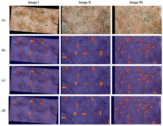
Figure 12.
Comparison of heat maps of ATD-YOLO, YOLOv8n, and YOLOv11n. (a) Original GT image; (b) YOLOv8n test results; (c) YOLOv11n test results; (d) ATD-YOLO test results.
To supplement the interpretability of the heat map model evaluation, this section uses four quantitative indicators: MAV, AE, BMA, and AC, for comparison. The results of the indicators are shown in Table 9.
Table 9.
Quantitative index.
The results show that ATD-YOLO performs best on image II, with the lowest AE (11.676), the highest AC (2.087), and the lowest BMA (0.277), reflecting the advantages of target feature concentration, strong background suppression, and an outstanding discrimination ability. YOLOv11n has an excellent performance in BMA (0.241) and AC (1.476) on image I, which is suitable for complex background scenes, but its AE is generally high, and feature concentration needs to be optimized. YOLOv8 n has the highest MAV (0.5) in image II, but the BMA (0.537) is also the highest, resulting in an AC (1.079) close to 1, and the target background discrimination ability is weak; meanwhile, the AC in image III is lower than 1, and the performance is significantly worse.
In summary, ATD-YOLO is better in feature concentration, background suppression, and discrimination. YOLOv11n is suitable for complex background scenes, while YOLOv8n needs to strengthen background noise suppression and target background contrast. These indicators provide a key basis for model interpretability analysis and performance optimization, help subsequent model improvement and scene adaptation, and provide data support for model selection and optimization in target detection tasks.
4. Discussion
In this study, the YOLOv8n model was improved. Considering the deployability and light weight of YOLOv8n, it was selected as the basic model. As described in Section 2, based on YOLOv8n, this study optimized the intra-scale feature interaction, channel-spatial attention mechanism, detector structure, model parameter quantity, and computational complexity and designed the ATD-YOLO model. To prove the effectiveness of each independent module, ablation experiments were performed, as shown in Table 3. The improved model is superior to the basic model in the training stage and the test stage. The performance of the model was proven by comparing the precision, recall rate, and mAP, as shown in Figure 9. To further intuitively observe the precision and generalization ability of other comparison models with the YOLO series, this paper presented a visual experiment, as shown in Figure 10 and Figure 11. Experiments show that by integrating an intra-scale feature interaction module (AIFI), a convolution block attention module (CBAM), and a lightweight shared convolution detection head (LTSC), the ATD-YOLO model improves the recognition ability under the challenges of a complex background and target occlusion, and it achieves higher detection precision in different distribution density scenarios.
Although this model shows a good performance in the controlled dataset environment, its robustness in extreme weather conditions (such as heavy rain, dust storms) or cross-species interference (such as other insect effects) scenarios still needs to be improved, and more field tests are needed to verify its practical application effect. Future research can combine edge computing devices to fully verify the real-time performance of the model in multi-modal data scenarios, to ensure its stability and reliability in complex real-world environments.
In terms of model accuracy and related indicators, it has been significantly improved compared with the past, but the experimental results have also exposed some problems that need to be solved urgently. As an important basis for model experiments, although this paper has simulated the distribution of locusts in real scenes as much as possible, there are still problems, such as an insufficient number of targets and uneven data quality. At the same time, the manual annotation process of the dataset may introduce uncertainties, which may lead to misclassification or labeling, with a certain impact on the training effect of the model.
In terms of model structural optimization, although ATD-YOLO has made phased progress in reducing the number of parameters and computational complexity, it is still necessary to explore more lightweight model structures and algorithms in order to further improve computational efficiency and maintain high-precision advantages. Through continuous optimization of model design, it is expected that researchers may achieve a more efficient computing performance in practical applications and promote the application of related technologies.
For agricultural communities, this study provides a practical and lightweight solution for locust monitoring, which can assist plant protection robots in preventing agricultural pests and diseases, thereby reducing the dependence on labor-intensive manual surveys and improving the disaster response efficiency. It is hoped that this research will promote the further development of field locust monitoring technology.
5. Conclusions
This paper presented a Locusta migratoria ssp. manilensis dataset focusing on real and complex backgrounds, a change in locust density, and a diversity of poses, which enriches the data resources and provides data support for locust monitoring in the future. At the same time, an optimization model, ATD-YOLO based on YOLOv8n, is proposed, which effectively improves the detection performance of locusts in complex environments. Firstly, the SPPF structure at the end of the original YOLOv8n network backbone is replaced, and the attention-based intra-scale feature interaction (AIFI) module is introduced to enhance the network’s ability to capture long-distance dependent information, thereby improving the detection precision of targets at different scales. Secondly, the channel-space attention module (CBAM) is integrated, which enables the network to adapt to complex backgrounds and improves the ability of the network to suppress background noise and highlight the expression ability of key areas. Thirdly, a lightweight shared convolution structure (LTSC) is proposed in the detection head part, which improves the parameter utilization efficiency of the detection head and enhances the recognition precision of locusts.
The experimental results show that the proposed model achieves a mean average precision (mAP) of 90.9% on the Real-Locust dataset, the precision is improved by 0.6%, the recall rate is improved by 4.3%, and the parameter quantity and computational complexity are reduced by 27.4% and 22.9%, respectively. These results show that the proposed method effectively handles the detection of locusts in complex environments and provides valuable technical support for their real-time monitoring.
Future work will focus on (1) expanding the dataset with a ground perspective and multi-angle UAV images, and combining Generative Adversarial Networks (GANs) to synthesize diverse locust scenes in order to enhance the generalization of the model; (2) exploring ultra-lightweight architectures through model pruning, quantization, or knowledge distillation to further reduce the computational overheads of resource-constrained edge devices; and (3) integrating ATD-YOLO into the intelligent agricultural system for real-time field deployment to achieve dynamic early warning and precise control of pests.
Author Contributions
Conceptualization, J.F., Y.Z., X.W. and P.W.; methodology, P.W.; software, P.W.; validation, J.F., P.W., X.W. and Y.Z.; formal analysis, P.W.; investigation, P.W.; writing—original draft preparation, P.W. and J.F.; writing—review and editing, P.W.; visualization, P.W.; supervision, J.F., X.W. and Y.Z.; project administration, J.F., X.W. and Y.Z.; funding acquisition, J.F. All authors have read and agreed to the published version of the manuscript.
Funding
This work was supported by the Inner Mongolia Scientific and Technological Project (Grant Nos. 2023YFJM0002, 2025KYPT0088) and funded by the Basic Research Operating Costs of Colleges and Universities directly under the Inner Mongolia Autonomous Region (Grant No. JY20240076).
Data Availability Statement
The data presented in this study are available on request from the corresponding author. The data are not publicly available due to an ongoing study.
Conflicts of Interest
The authors declare no conflicts of interest.
References
- Wang, X.; Li, G.; Wang, S.; Feng, C.; Xu, W.; Nie, Q.; Liu, Q. The effect of environmental changes on locust outbreak dynamics in the downstream area of the Yellow River during the Ming and Qing Dynasties. Sci. Total Environ. 2023, 877, 162921. [Google Scholar] [CrossRef]
- Yao, X.; Zhu, D.; Yun, W.; Peng, F.; Li, L. A WebGIS-based decision support system for locust prevention and control in China. Comput. Electron. Agric. 2017, 140, 148–158. [Google Scholar] [CrossRef]
- Khan, I.; Ullah, W.; Karamic, A.; Qazid, I.; Ahamade, I. Analyze the Socioeconomic Consequences of Locust Outbreaks on Agriculture, Rural Communities, And Food Security. Indus J. Anim. Plant Sci. 2023, 1, 15–20. [Google Scholar]
- Latchininsky, A.V. Locusts and remote sensing: A review. J. Appl. Remote Sens. 2013, 7, 075099. [Google Scholar] [CrossRef]
- Ye, S.; Lu, S.; Bai, X.; Gu, J. ResNet-Locust-BN Network-Based Automatic Identification of East Asian Migratory Locust Species and Instars from RGB Images. Insects 2020, 11, 458. [Google Scholar] [CrossRef]
- Zhao, L.; Huang, W.; Chen, J.; Dong, Y.; Ren, B.; Geng, Y. Land use/cover changes in the Oriental migratory locust area of China: Implications for ecological control and monitoring of locust area. Agric. Ecosyst. Environ. 2020, 303, 107110. [Google Scholar] [CrossRef]
- Wang, X.; Fan, J.; Zhou, M.; Gao, G.; Wei, L.; Kang, L. Interactive effect of photoperiod and temperature on the induction and termination of embryonic diapause in the migratory locust. Pest Manag. Sci. 2021, 77, 2854–2862. [Google Scholar] [CrossRef]
- Gómez, D.; Salvador, P.; Sanz, J.; Rodrigo, J.F.; Gil, J.; Casanova, J.L. Prediction of desert locust breeding areas using machine learning methods and SMOS (MIR_SMNRT2) Near Real Time product. J. Arid Environ. 2021, 194, 104599. [Google Scholar] [CrossRef]
- Tabar, M.; Gluck, J.; Goyal, A.; Jiang, F.; Morr, D.; Kehs, A.; Lee, D.; Hughes, D.P.; Yadav, A. A PLAN for Tackling the Locust Crisis in East Africa: Harnessing Spatiotemporal Deep Models for Locust Movement Forecasting. In Proceedings of the Proceedings of the 27th ACM SIGKDD Conference on Knowledge Discovery & Data Mining, Singapore, 14–18 August 2021; pp. 3595–3604. [Google Scholar] [CrossRef]
- Kimathi, E.; Tonnang, H.E.Z.; Subramanian, S.; Cressman, K.; Abdel-Rahman, E.M.; Tesfayohannes, M.; Niassy, S.; Torto, B.; Dubois, T.; Tanga, C.M.; et al. Prediction of breeding regions for the desert locust Schistocerca gregaria in East Africa. Sci. Rep. 2020, 10, 11937. [Google Scholar] [CrossRef]
- Shao, Z.; Feng, X.; Bai, L.; Jiao, H.; Zhang, Y.; Li, D.; Fan, H.; Huang, X.; Ding, Y.; Altan, O.; et al. Monitoring and Predicting Desert Locust Plague Severity in Asia–Africa Using Multisource Remote Sensing Time-Series Data. IEEE J. Sel. Top. Appl. Earth Obs. Remote Sens. 2021, 14, 8638–8652. [Google Scholar] [CrossRef]
- Sun, R.; Huang, W.; Dong, Y.; Zhao, L.; Zhang, B.; Ma, H.; Geng, Y.; Ruan, C.; Xing, N.; Chen, X.; et al. Dynamic Forecast of Desert Locust Presence Using Machine Learning with a Multivariate Time Lag Sliding Window Technique. Remote Sens. 2022, 14, 747. [Google Scholar] [CrossRef]
- Guo, J.; Zhao, L.; Huang, W.; Dong, Y.; Geng, Y. Study on the Forming Mechanism of the High-Density Spot of Locust Coupled with Habitat Dynamic Changes and Meteorological Conditions Based on Time-Series Remote Sensing Images. Agronomy 2022, 12, 1610. [Google Scholar] [CrossRef]
- Gerakari, M.; Katsileros, A.; Kleftogianni, K.; Tani, E.; Bebeli, P.J.; Papasotiropoulos, V. Breeding of Solanaceous Crops Using AI: Machine Learning and Deep Learning Approaches—A Critical Review. Agronomy 2025, 15, 757. [Google Scholar] [CrossRef]
- Bai, Z.; Tang, Z.; Diao, L.; Lu, S.; Guo, X.; Zhou, H.; Liu, C.; Li, L. Video target detection of East Asian migratory locust based on the MOG2-YOLOv4 network. Int. J. Trop. Insect Sci. 2022, 42, 793–806. [Google Scholar] [CrossRef]
- Liu, L.; Liu, M.; Meng, K.; Yang, L.; Zhao, M.; Mei, S. Camouflaged locust segmentation based on PraNet. Comput. Electron. Agric. 2022, 198, 107061. [Google Scholar] [CrossRef]
- Kamalesh, K.S.; Kumaraperumal, R.; Pazhanivelan, P.; Jagadeeswaran, R.; Prabu, P.C. YOLO deep learning algorithm for object detection in agriculture: A review. J. Agric. Eng. 2024, 55, 1641. [Google Scholar] [CrossRef]
- Li, P.; Zhou, J.; Sun, H.; Zeng, J. RDRM-YOLO: A High-Accuracy and Lightweight Rice Disease Detection Model for Complex Field Environments Based on Improved YOLOv5. Agriculture 2025, 15, 479. [Google Scholar] [CrossRef]
- Liu, Z.; Guo, X.; Zhao, T.; Liang, S. YOLO-BSMamba: A YOLOv8s-Based Model for Tomato Leaf Disease Detection in Complex Backgrounds. Agronomy 2025, 15, 870. [Google Scholar] [CrossRef]
- Zhang, W.; Huang, H.; Sun, Y.; Wu, X. AgriPest-YOLO: A rapid light-trap agricultural pest detection method based on deep learning. Front. Plant Sci. 2022, 13, 1079384. [Google Scholar] [CrossRef]
- Zhu, L.; Li, X.; Sun, H.; Han, Y. Research on CBF-YOLO detection model for common soybean pests in complex environment. Comput. Electron. Agric. 2024, 216, 108515. [Google Scholar] [CrossRef]
- Wang, N.; Fu, S.; Rao, Q.; Zhang, G.; Ding, M. Insect-YOLO: A new method of crop insect detection. Comput. Electron. Agric. 2025, 232, 110085. [Google Scholar] [CrossRef]
- Yu, Y.; Zhou, Q.; Wang, H.; Lv, K.; Zhang, L.; Li, J.; Li, D. LP-YOLO: A Lightweight Object Detection Network Regarding Insect Pests for Mobile Terminal Devices Based on Improved YOLOv8. Agriculture 2024, 14, 1420. [Google Scholar] [CrossRef]
- LabelImg. Available online: https://github.com/tzutalin/labelimg (accessed on 26 May 2025).
- Wang, C.; Wang, L.; Ma, G.; Zhu, L. CSF-YOLO: A Lightweight Model for Detecting Grape Leafhopper Damage Levels. Agronomy 2025, 15, 741. [Google Scholar] [CrossRef]
- Yang, L.; Zhang, T.; Zhou, S.; Guo, J. AAB-YOLO: An Improved YOLOv11 Network for Apple Detection in Natural Environments. Agriculture 2025, 15, 836. [Google Scholar] [CrossRef]
- Varghese, R.; Sambath, M. YOLOv8: A Novel Object Detection Algorithm with Enhanced Performance and Robustness. In Proceedings of the 2024 International Conference on Advances in Data Engineering and Intelligent Computing Systems (ADICS), Chennai, India, 18–19 April 2024; pp. 1–6. [Google Scholar] [CrossRef]
- Zhao, Y.; Lv, W.; Xu, S.; Wei, J.; Wang, G.; Dang, Q.; Liu, Y.; Chen, J. Detrs beat yolos on real-time object detection. In Proceedings of the IEEE/CVF Conference on Computer Vision and Pattern Recognition, Seattle, WA, USA, 16–22 June 2024. [Google Scholar] [CrossRef]
- Chen, L.; Li, G.; Zhang, S.; Mao, W.; Zhang, M. YOLO-SAG: An improved wildlife object detection algorithm based on YOLOv8n. Ecol. Inform. 2024, 83, 102791. [Google Scholar] [CrossRef]
- Liu, R.; Huang, M.; Wang, L.; Bi, C.; Tao, Y. PDT-YOLO: A Roadside Object-Detection Algorithm for Multiscale and Occluded Targets. Sensors 2024, 24, 2302. [Google Scholar] [CrossRef]
- Guo, M.-H.; Xu, T.-X.; Liu, J.-J.; Liu, Z.-N.; Jiang, P.-T.; Mu, T.-J.; Zhang, S.-H.; Martin, R.R.; Cheng, M.-M.; Hu, S.-M. Attention mechanisms in computer vision: A survey. Comput. Vis. Media 2022, 8, 331–368. [Google Scholar] [CrossRef]
- Woo, S.; Park, J.; Lee, J.Y.; Kweon, I.S. CBAM: Convolutional Block Attention Module. In Computer Vision—ECCV 2018; Ferrari, V., Hebert, M., Sminchisescu, C., Weiss, Y., Eds.; Lecture Notes in Computer Science; Springer: Berlin/Heidelberg, Germany, 2018; Volume 11211. [Google Scholar] [CrossRef]
- Chen, J.; Liu, R.; Tong, Y.; Wu, H. Synthetical application of multi-feature map detection and multi-branch convolution. J. Wirel. Commun. Netw. 2019, 125. [Google Scholar] [CrossRef]
- Cheng, X.; Yu, J. RetinaNet with Difference Channel Attention and Adaptively Spatial Feature Fusion for Steel Surface Defect Detection. IEEE Trans. Instrum. Meas. 2021, 70, 2503911. [Google Scholar] [CrossRef]
- Tian, Z.; Shen, C.; Chen, H.; He, T. FCOS: Fully Convolutional One-Stage Object Detection. In Proceedings of the 2019 IEEE/CVF International Conference on Computer Vision (ICCV), Seoul, Republic of Korea, 27 October–2 November 2019; pp. 9626–9635. [Google Scholar] [CrossRef]
- Tian, Y.; Ye, Q.; Doermann, D. Yolov12: Attention-centric real-time object detectors. arXiv 2025, arXiv:2502.12524. [Google Scholar]
- Chattopadhay, A.; Sarkar, A.; Howlader, P.; Balasubramanian, V.N. Grad-CAM++: Generalized Gradient-Based Visual Explanations for Deep Convolutional Networks. In Proceedings of the 2018 IEEE Winter Conference on Applications of Computer Vision (WACV), Lake Tahoe, NV, USA, 12–15 March 2018; pp. 839–847. [Google Scholar] [CrossRef]
Disclaimer/Publisher’s Note: The statements, opinions and data contained in all publications are solely those of the individual author(s) and contributor(s) and not of MDPI and/or the editor(s). MDPI and/or the editor(s) disclaim responsibility for any injury to people or property resulting from any ideas, methods, instructions or products referred to in the content. |
© 2025 by the authors. Licensee MDPI, Basel, Switzerland. This article is an open access article distributed under the terms and conditions of the Creative Commons Attribution (CC BY) license (https://creativecommons.org/licenses/by/4.0/).