Impact of a Saline Soil Improvement Project on the Spatiotemporal Evolution of Groundwater Dynamic Field and Hydrodynamic Process Simulation in the Hetao Irrigation District

Abstract

This study examined groundwater dynamics under saline–alkali improvement measures in a 3.66 × 10⁷ m² study area in Wuyuan County, Hetao Irrigation District, where agricultural sustainability is constrained by soil salinization. This work investigated the spatiotemporal evolution patterns and influencing factors of the groundwater environment in the context of soil salinity–alkalinity improvement, as well as the impact of irrigation on the ionic characteristics of groundwater. Furthermore, based on this analysis, a groundwater numerical model and a prediction model for the study area were developed using Visual MODFLOW Flex 6.1 software to forecast the future groundwater levels in the study area and evaluate the effects of varying irrigation scenarios on these levels. The key findings are as follows: (1) The groundwater depth stabilized at 1.63 ± 0.15 m (0.4 m increase) post-improvement measures, maintaining equilibrium under current irrigation but increasing with reductions in water supply. The groundwater salinity increased by 0.59–1.2 g/L across the crop growth period. (2) Spring irrigation raised the groundwater total dissolved solids by 15.6%, as influenced by rock weathering (38.2%), evaporation (31.5%), and cation exchange (30.3%). (3) Maintaining current irrigation systems and planting structures could stabilize groundwater levels at 1.60–1.65 m over the next decade, confirming the sustainable hydrological effects of soil improvement measures. Reducing irrigation to 80% of the current water supply of the Yellow River enables groundwater level stabilization (2.05 ± 0.12 m burial depth) within 5–7 years. This approach decreases river water dependency by 20% while boosting crop water efficiency by 18.7% and reducing root zone salt stress by 32.4%.

1. Introduction

Planned water allocation measures have been implemented in the Yellow River under a China-unified water resource management strategy [1,2]. Since 1998, the annual diversions in the Yellow River have decreased from 5.2 to 4.7 billion m³, with the Hetao Irrigation District’s quota set to reduce this figure to 4 billion m³ by 2010, thus intensifying water supply–demand [3]. As one of China’s three major gravity-fed irrigation zones, Inner Mongolia’s Hetao Irrigation District covers 1.162 million hm² [4]. This saline–alkali region in the Yellow River’s mid-upper reaches is characterized by low rainfall and high evaporation (vapor deficit > 10) [5]; as a result, reducing the use of irrigation water is critical to ecosystem health in this region [6]. In 2018, Wuyuan County initiated a 3.66 × 10⁷ m² salinity reduction and grassland enhancement pilot, combining various water conservation, agricultural, and forestry measures, such as strip cultivation, land leveling, chemical/organic soil improvement, subsurface drainage, channel maintenance, and deep tillage. These interventions have significant impacts on local groundwater systems [7]. Adverse impacts on groundwater are hard to detect owing to the considerably very slow movement of groundwater, which results in a lack of proper knowledge and information about the future implications of climate change and other anthropogenic activities [8]. Therefore, it is highly necessary to assess the pollution and flow conditions of groundwater through powerful and effective technical means.

Soil salinization is caused by both natural and human factors and severely constrains agricultural production and ecological sustainability [9,10]. In the Hetao Irrigation District, over 330,000 hm² of its 530,000 hm² irrigated land faces threats from salinization, with the proportion of affected areas expanding by 1–3% annually over the last 30 years [11]. In this region, secondary salinization primarily results from highly mineralized groundwater and rising water tables [12,13]. Understanding the spatiotemporal patterns of groundwater is crucial for salinization control [14]. Current groundwater research employs methods [15] such as geostatistics, isotopic tracing [16], and hydrogeological simulation [17], alongside spatial interpolation techniques such as Kriging and the inverse distance weighting method, which are widely used in analyzing the evolution of regional groundwater and soil salinity [18]. Using the same amount of data, Kriging generally achieves lower prediction errors compared to the inverse distance weighting method (IDW), especially in scenarios with complex spatial structures (such as terrain elevation analysis), where the advantage is particularly significant. In simulation studies [19], the root mean square error of Kriging is 10% to 30% lower than that of IDW, especially in areas with sparse data.

Following sustained advancements in computational capabilities and over two decades of global research and development, groundwater numerical modeling techniques have achieved significant technological maturation [20]. The field has witnessed the emergence of numerous influential numerical models and specialized software suites that continue to serve as indispensable resources in contemporary hydrogeological investigations. Internationally recognized platforms such as Visual MODFLOW, FEFLOW, and GMS maintain their prominence in groundwater simulation research, demonstrating enduring scientific relevance and practical application value [21,22]. Current research focuses on addressing simulation challenges using advanced mathematics tools to model uncertainties across scales [23]. Shu et al. [24] conducted a study on the impact of agricultural irrigation and the South-to-North Water Diversion Project on the dynamic changes in groundwater in the Shijiazhuang Plain area through hydrological models. Diao et al. [25] established a numerical simulation model for the northern part of Weifang using Visual MODFLOW, analyzed and predicted the water supply and demand volumes for the planning year, and formulated a water resource optimization allocation plan. Ye et al. [26] adopted the method of quota management for well water intake volume, based on the hydrogeological model software GMS, and conducted a simulation study on the groundwater level in the demonstration area.

Intensifying groundwater needs alongside the incessantly degrading quality of groundwater in numerous areas around the globe urges prompt actions to reinforce the global-scale adequate management of groundwater. Some groups of scholars focused on conducting research in specific areas, using methods such as the water balance model, eco-hydrological models, and groundwater flow models. Kassem et al. [27] established an integrated validated numerical groundwater model of a karst catchment area (Lebanon), which is used to evaluate the impact of model parameters on recharge and spring discharge and identify important parameters that control the intrinsic system vulnerability. Based on the results, this method proposes re-evaluating the weighting coefficients of key vulnerability factors in the conventional methods based on a numerical model for the establishment of water protection guidelines. Lin et al. [28] employed the theory of imperfect interfaces to model groundwater flow at the fault–aquifer interface, replacing the simplified source-term approximations commonly used in previous analytical models. Peters et al. [29] introduced the hydrological model SALTFRED to describe and comprehend the soil water processes and their dynamics in tropical saltmarshes. This model aims to mechanistically predict soil water salinity and root zone soil moisture, elucidating the intricate differentiation of drought and salt stress within the saltmarsh. The model explicitly describes processes of infiltration, seepage, and evapotranspiration, along with their influence on the salinity of the soil water. However, implementing such models and parameterizing them with field measurements is highly demanding. Simultaneously, we strive for a simple and easy-to-use implementation to promptly reflect the groundwater conditions of the area and provide a reference for future management.

It can be seen from previous studies that scholars have mostly analyzed the dynamic changes in groundwater in local areas based on models and combined with historical observational data, rarely conducting studies on the overall groundwater dynamic changes in an entire region. Secondly, in the established groundwater models of the entire area, there is a lack of research on long-term sequence and regional-scale changes in groundwater and soil salinity as well as the influencing factors. At the same time, due to the joint influence of precipitation, evaporation, and groundwater level on farmland in irrigation areas and the cross-coupling of various influencing factors, the complexity and variability of regional water–salt transport increase. Moreover, the implementation of large-scale soil salinity improvement projects has led to significant changes in the water cycle and groundwater depth in the irrigation area. Therefore, it is necessary to carry out quantitative simulations of regional-scale groundwater and analyses of influencing factors as well as long-term sequence prediction analyses, clarifying the spatiotemporal evolution laws of the groundwater environment under the influencing factors of soil salinity improvement and their impact on groundwater ion characteristics.

In order to study the spatiotemporal evolution laws and influencing factors of the groundwater environment after the implementation of soil salinization and alkalization improvement projects, this study monitored groundwater depth and quality in a 3.66 × 10⁷ m² saline–alkali land improvement area, analyzing the spatiotemporal patterns of groundwater depth, mineralization, and quality. Furthermore, based on the hypothesis that soil improvement measures will stabilize the groundwater level, the groundwater numerical model and prediction model were developed using Visual MODFLOW Flex 6.1 software for the Hetao Irrigation District based on hydrogeological conditions. Automated monitoring enhanced model accuracy by clarifying groundwater volume exchange. This research also evaluated water balance, predicted groundwater levels, and assessed the impacts of irrigation on water tables. By establishing this numerical model, this paper explores how large-scale land improvement affects groundwater environments and predicts future impacts, providing data support for saline–alkali land remediation projects.

2. Materials and Methods

2.1. Application Scheme

This study examined the “Salt Conversion and Grass Enhancement” project (54,828 mu) in Longxingchang Town, Wuyuan County, Inner Mongolia. It investigated groundwater environmental impacts under saline–alkali soil improvement initiatives. We based this on the hypothesis that soil improvement measures will stabilize the groundwater level. Combining statistical analysis, geostatistics, and hydrogeological methods, the research reveals the spatiotemporal evolution patterns of groundwater dynamics and chemistry pre/post-soil treatment. A Visual MODFLOW-based 3D groundwater flow model(Waterloo Hydrogeology Company, Waterloo, Ontario, Canada) is used to simulate the responses of shallow aquifers under various irrigation scenarios, offering scientific support for optimizing water allocation and evaluating the effects on the groundwater environment.

(1)

Groundwater Dynamics Pre- and Post-Improvement Project

An analysis of 2018–2021 monitoring data was conducted, employing classical statistics, geostatistics, and spatial interpolation analyses. Research was conducted to reveal spatiotemporal variations in groundwater depth and key controlling factors. Post-remediation groundwater quality was evaluated using an Inverted Nemerow Pollution Index and the salinity and alkalinity evaluation method, integrating pollution severity, salinization hazards, and composite risk indices.

(2)

Irrigation-Driven Water–Salt Regulation Mechanisms

Hydrochemical parameters (pH and major ions) and soil profile conductivity from 2021 irrigation cycles were analyzed via Piper diagrams, Gibbs plots, and Pearson correlation. The results showed irrigation-induced shifts in groundwater chemistry as well as coupled mechanisms of salt transport and salt accumulation at the soil–water interface.

(3)

Regional Groundwater Model Development and Validation

Through the systematic compilation of hydrogeological and meteorological datasets from the studied region, coupled with the synthesis of revised boundary constraints, anthropogenic modifications to field infrastructure, and historical groundwater dynamics, a comprehensive conceptual hydrogeological framework was constructed employing the Visual MODFLOW computational platform. Following the rigorous integration of the initial hydraulic parameters and the quantification of source–sink components, this conceptual framework was subsequently transformed into a high-resolution numerical groundwater model, which underwent calibration and validation procedures to ensure its predictive reliability.

(4)

Groundwater Level Projections and Irrigation Scenario Analysis

Following rigorous model calibration, simulations of the baseline (current irrigation) and water-saving scenarios (10–30% reductions) were used to obtain groundwater responses for the 2025–2030 period. The water table fluctuation method quantified infiltration recharge coefficients, establishing irrigation volume–groundwater level linkage equations.

2.2. General Introduction to the Study Area

2.2.1. Study Areas

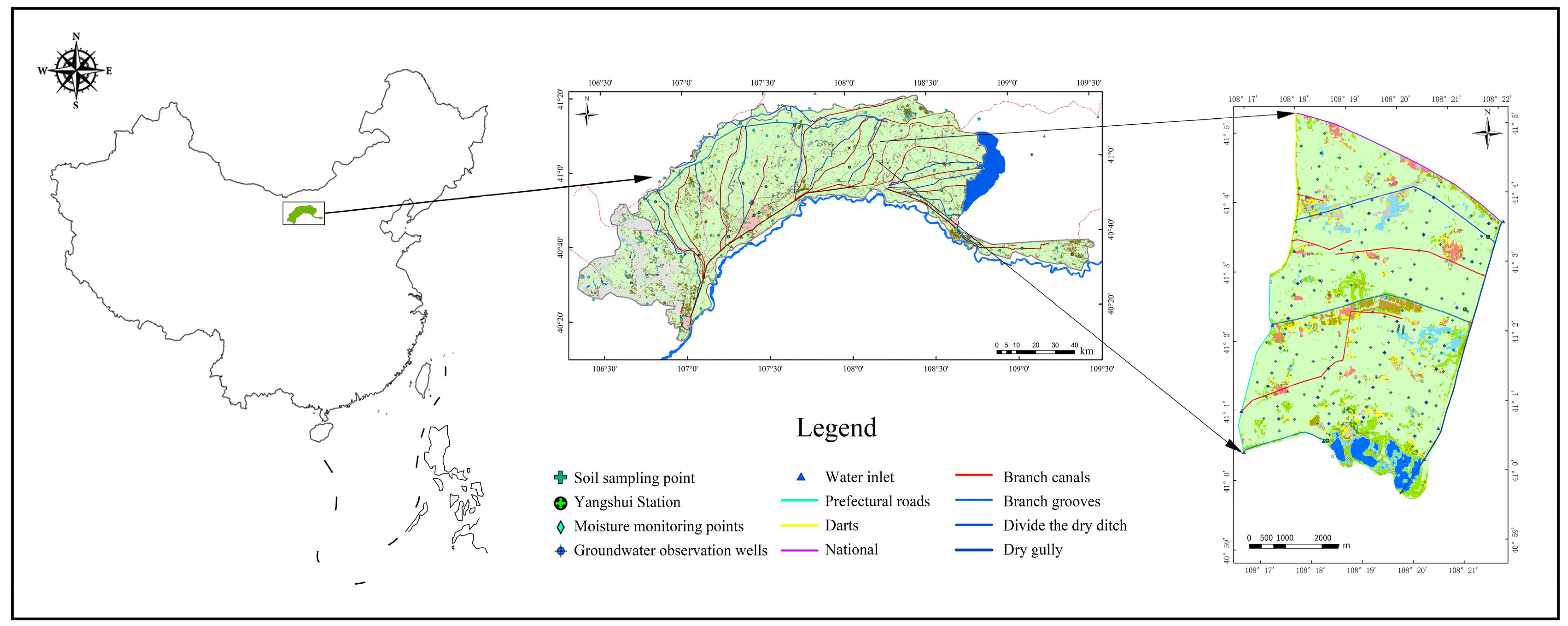
The study area lies in the central Hetao Plain, south of the Yellow River and north of the Yinshan Mountains. It encompasses the downstream Yichang Irrigation District in Bayannur City, Inner Mongolia, specifically within Wuyuan County’s livestock development demonstration zone. Covering 3.66 × 10⁷ m², the area measures approximately 5.76 km east–west and 9.07 km north–south. Its boundaries include the National Highway 110 (north), Mengwangshuan West Zhonghai (south), Provincial Road S212 (west), and Yitong Drainage (east). Its coordinates span 107°35′70″–108°37′50″ E longitude and 40°46′30″–41°16′45″ N latitude. Its geographical features are shown in Figure 1.

2.2.2. Elevation of the Study Area

The elevation of the study area ranges from 1019.97 to 1023.96 m, with the south being higher than the north, the west higher than the east, and the central region relatively lower compared to the southern and northern parts. The highest point is located in the southwest, reaching an altitude of 1023.96 m, while the lowest point is in the western center, at an altitude of 1019.97 m. The terrains in the south, the central region, and the north are higher in the southwest and lower in the southeast, the central region is higher in the west and lower in the east, and the north is lower in the northeast, respectively.

2.2.3. Climate Overview

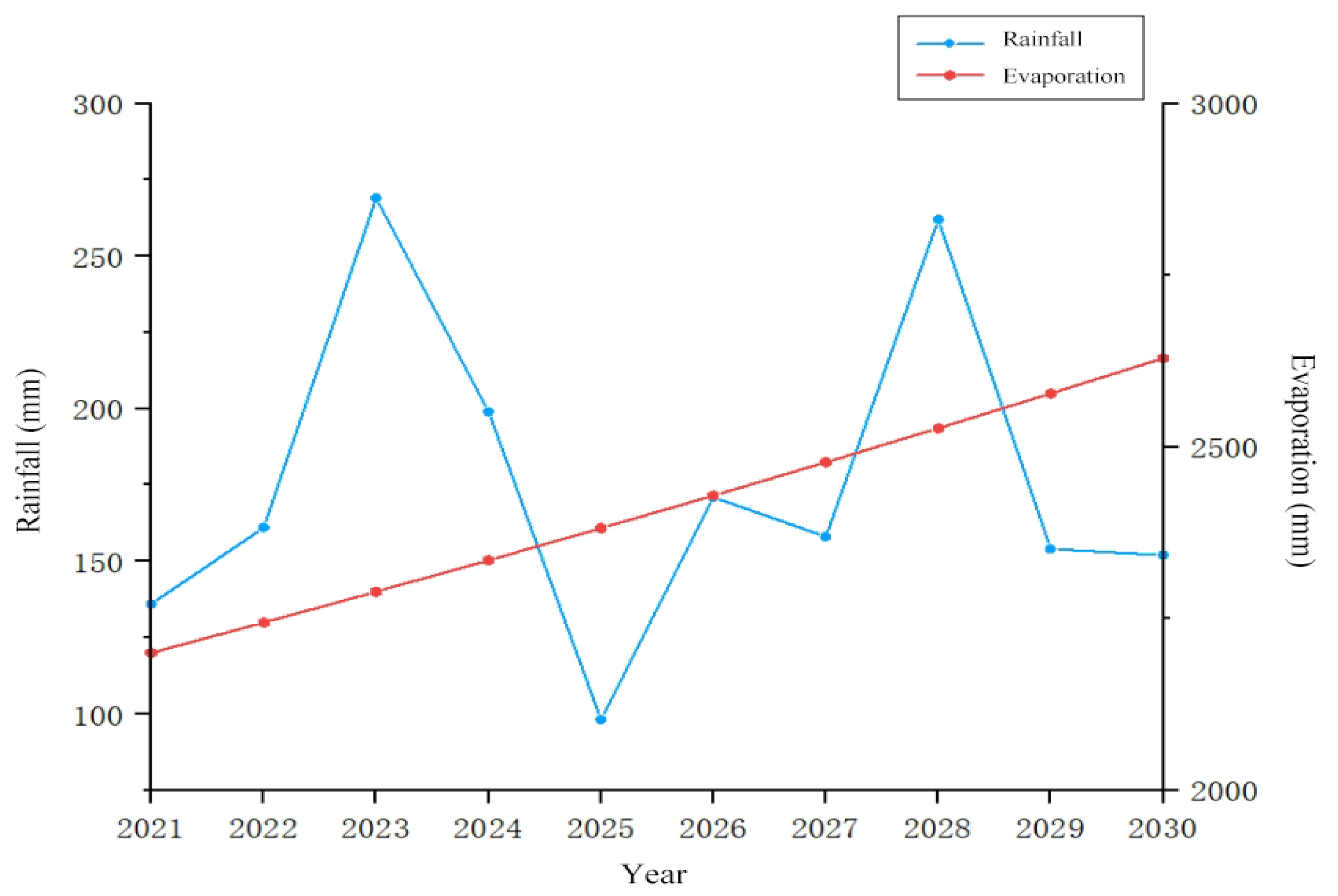
The study area features a temperate continental climate with abundant light/heat, long periods of sunshine, dry air, high winds, large diurnal temperature variations, and low rainfall. Annual solar radiation reaches 153.44 kcal/cm², with precipitation averaging 136.8–213.5 mm against evaporation levels of 1993–2372 mm, yielding a 10:1 evapotranspiration ratio. Evaporation in May–July exceeds 50% of the annual total, intensifying water–heat imbalances [30]. Increases in evaporation during summer correlate with rises in temperature and decreases in rainfall [31]. Precipitation markedly varies interannually: wet years (2001, 2008, 2013, and 2017) surpass multi-year averages, while dry years (2000, 2007, 2009, 2019, and 2021) fall below them. The East Asian monsoon drives uneven intra-annual distribution—85% of the rainfall occurs in June–November (63–70% in June–August), with spring (March–May) contributing merely 10–20%. Mean annual temperatures range from 6.3 to 7.7 °C, peaking in July and reaching their lowest in January, which is consistent with continental climate patterns in the Northern Hemisphere [32].

2.2.4. Hydrogeological Conditions

The lithology of the groundwater aquifer mainly consists of medium-fine sand and silt, transitioning from lacustrine to alluvial facies with thickness increasing from east to west and south to north. Wuyuan County’s alluvial–lacustrine plain contains two aquifer groups: The first (alluvial–lacustrine) lies above the lacustrine layer with 50–90 m thick silt sand, yielding 50–80 m³/h flow but with poor water quality. The second (alluvial confined) shows regional variations, generally having poor quality with 2–3 m capillary barriers at 70–90 m depth. Groundwater forms primarily through Yellow River irrigation infiltration (>80% recharge) and precipitation. Flow conditions depend on the characteristics of the terrain, climate, and aquifer, exhibiting low hydraulic gradient and vertical infiltration–evaporation cycles due to the Hetao Plain’s flat topography [33,34,35]. The seasonal dynamics reflect meteorological influences and irrigation patterns [36].

2.3. Data Collection

2.3.1. Field Observation Data

This study employs fixed-point groundwater monitoring. The groundwater well positions are determined based on the size of the actual elevation difference and the different planting structures of the farmland. At the locations of the irrigation and drainage ditches and adjacent areas in the field in the project area, one groundwater monitoring well is arranged approximately every one kilometer. The well positions are arranged in a rectangular pattern, forming a grid of 30 observation wells (Figure 1 and Figure S1). Starting from the observation wells as the sampling points, soil sampling points were set at intervals of about 300 m, totaling 149 soil sampling points. Indicators such as soil moisture content and salt content were measured. In 2018–2019, water and soil samples were collected from the groundwater observation wells and surrounding plots in April, June, and October each year. From 2020 to 2021, water and soil samples were collected from the groundwater observation wells and surrounding plots every month from April to October. HOBO water level meters continuously record groundwater levels year-round, with monthly verification from April to September.

Automatic flow and conductivity monitors are installed in the study area channels and ditches to track the volume and salinity of incoming and drainage water. Integrated monitoring devices measure the water volume, quality, and level at 4 intake points, 5 drainage inlets, and 1 outlet. Real-time data are collected through sensors and verified via custom water sampling buckets. A water level recorder at Tianlai Lake monitors water level/salinity. Observation Well No. 16 in the northern soil zone uses a three-parameter meter to track groundwater conductivity, level, and temperature.

2.3.2. Determination of Test Indicators

(1) Soil conductivity: Samples collected using a soil drill were measured in a 1:5 soil–water extract using a conductivity meter (DDS-307A, Shanghai Youke Instruments, Shanghai, China). Measurements spanned a depth of 0–100 cm across five 20 cm layers (0–20, 20–40, 40–60, 60–80, and 80–100 cm).

(2) The PVC observation well (110 mm diameter, 6 m length) was vertically buried at 5 m depth, with perforated filter cloth-wrapped sections. Groundwater depth was automatically recorded every 6 h using a self-installed gauge (HOBO U20-001-01, Onset Computer Corporation, Cape Cod, MA, USA), while manual monthly calibrations complemented real-time HOBO measurements.

(3) TDS of groundwater: TDS (total dissolved solids) is the total dissolved solid content of groundwater. The test method employed to measure TDS was steam determination.

(4) The eight major groundwater ions were analyzed using the following methods: Na⁺ and K⁺ were analyzed via spectrophotometry; Ca²⁺ and Mg²⁺ using EDTA titration; carbonates/bicarbonates through acid titration; Cl⁻ with silver nitrate titration; and SO₄²⁻ via EDTA titration.

(5) pH value and EC value of groundwater: The pH value was measured using a pH instrument (PHS-3C pH meter, Zhengzhou Baojing Electronic Technology, Zhengzhou, China) and the EC value was measured using a conductivity meter (DDSJ-308A Conductivity Meter, Shanghai Leici, Shanghai, China).

(6) Integrated ultrasonic flowmeters and conductivity monitors (Ultrasonic flowmeter SZ-DPL, Shanghai Shouxiao, Shanghai, China) were installed at the study area’s inlet/outlet to automatically collect flow and EC data. Irrigation water was lab-tested for soil salinity (EC) and the eight major ions, thus validating the automatic monitoring data.

3. Results

3.1. Groundwater Dynamics Pre- and Post-Improvement

3.1.1. Temporal Evolution of Groundwater Burial Depth

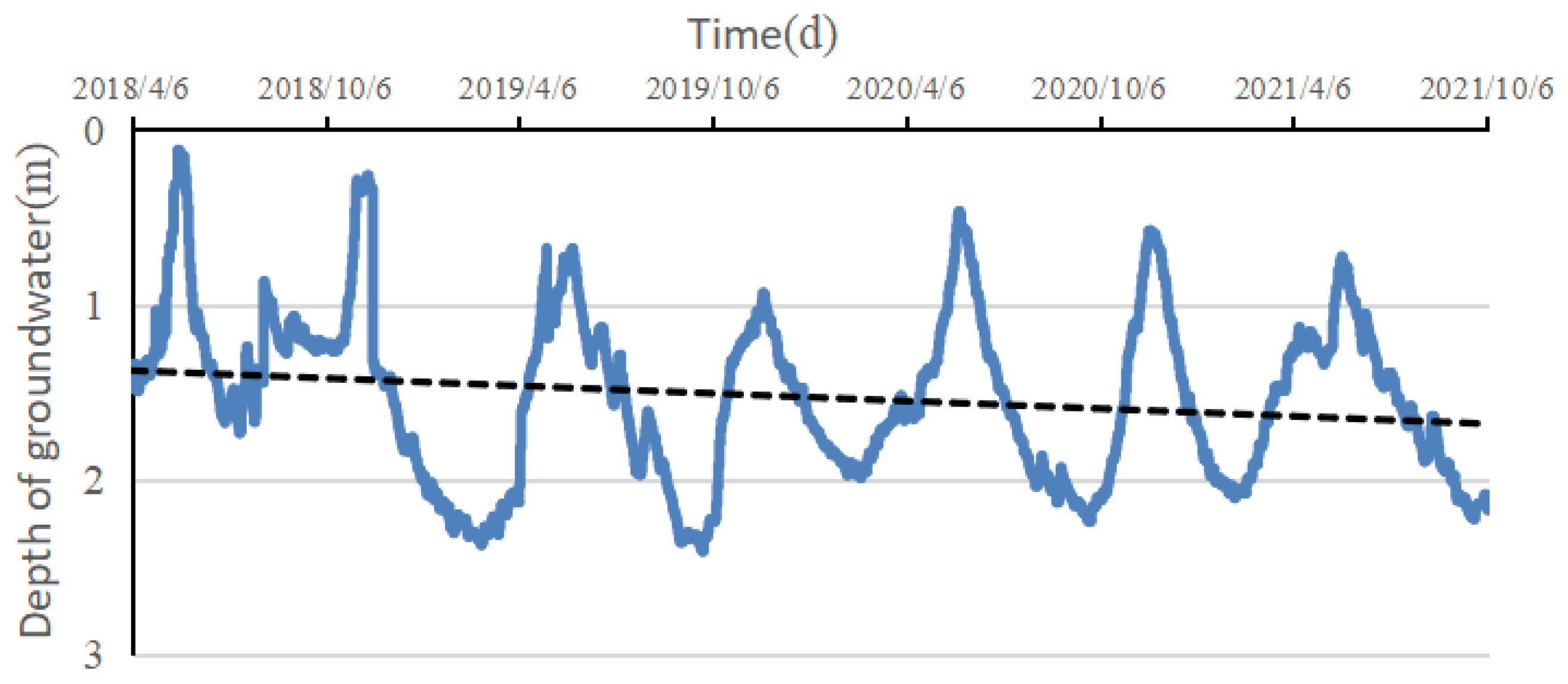
As shown in Figure 2 and Figure S2, following improvement measures such as the renovation of field water conservation infrastructure, land leveling, channel lining, and ditch dredging in the study area, the groundwater level declined and the groundwater burial depth showed an increasing trend. According to Table S1, the average annual groundwater burial depth changes within the range of 1.589–1.686 m after soil improvement due to minor differences in annual irrigation volume and variations in rainfall, stabilizing at around 1.63 m. There is a more significant decrease in the average annual groundwater burial depth post-soil improvement compared to before.

3.1.2. Analysis of Factors Influencing Groundwater Burial Depth

The study area is situated in the Hetao Irrigation District’s Yichang Domain. Annual spring irrigation with Yellow River water starts in mid-April using flooding methods. Planting begins 1–2 months post-irrigation, followed by crop growth. Sunflower cultivation dominates (71%), followed by corn (24%); the remainder comprises minor economic crops such as watermelon and tomatoes. Sunflower fields receive concentrated spring/autumn irrigation, while corn receives monthly irrigation during its growth. A period of high autumn irrigation occurs post-harvest in late October, initiating freeze–thaw cycles. Hydrological years are divided into freeze–thaw (November–April), spring irrigation/planting (April–mid-June), and crop growth (mid-June–October) cycles.

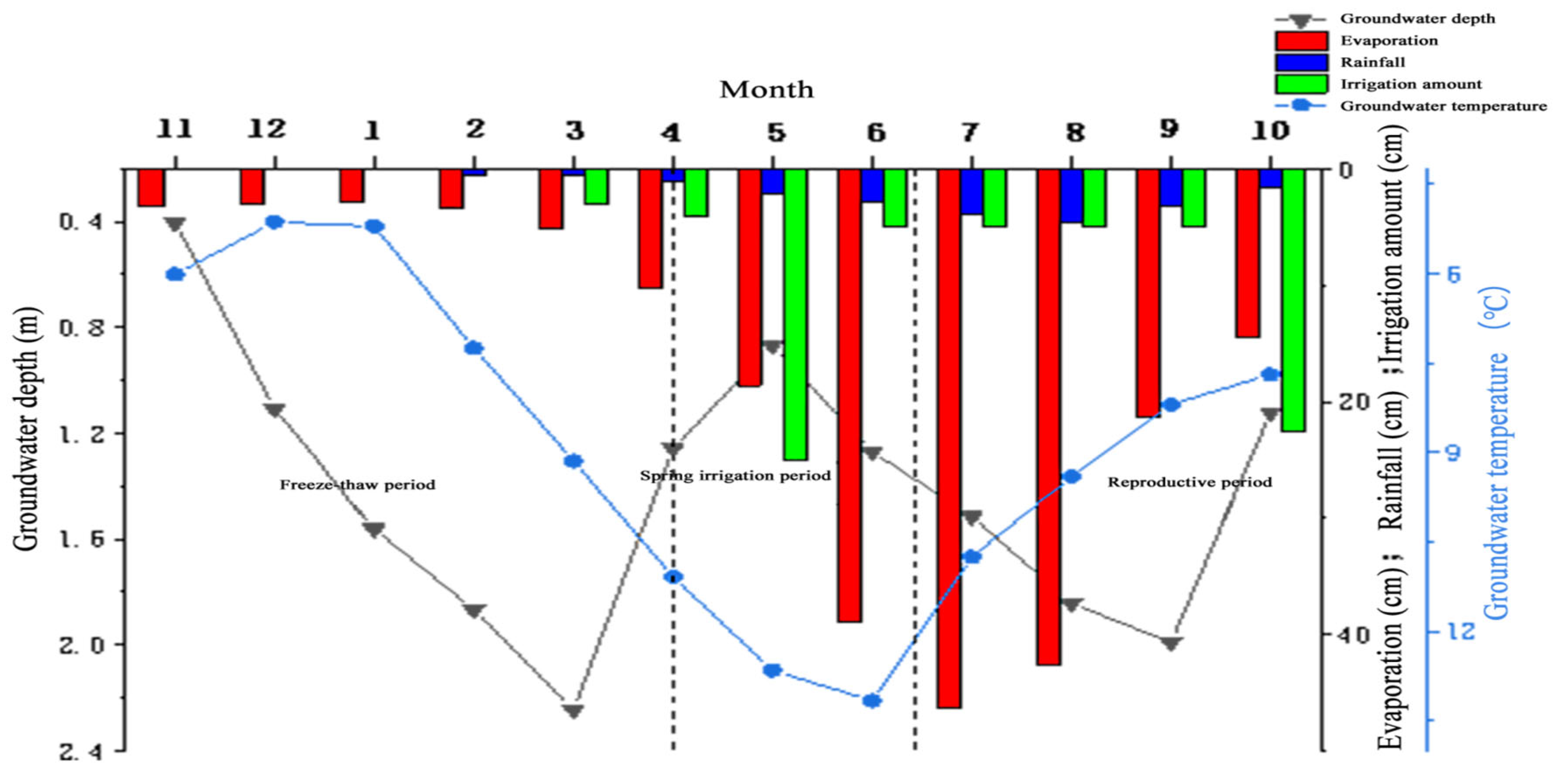
Monitoring data from the 2020–2021 period establish temporal patterns of groundwater depth, temperature, evaporation, rainfall, and irrigation. Figure 3 reveals significantly lower precipitation compared to irrigation and evaporation in the study area, indicating the minimal impact of precipitation on groundwater dynamics. Regional groundwater depth displays a bimodal annual pattern, with trough periods coinciding with spring/autumn irrigation peaks, confirming that irrigation regulation is the dominant controlling factor. The groundwater level reaches its maximum depth in March due to the cumulative effect of frozen soil layers during the freezing period. As the thickness of the frozen layer peaks at the end of the freezing period, the groundwater depth also reaches its highest. During thawing seasons, melted ice replenishes groundwater, causing continuous depth reduction until the end of spring irrigation.

The second groundwater depth peak occurs from September to October (post-harvest and pre-autumn irrigation). Post-spring irrigation, crops enter growth stages with only sporadic sunflower field irrigation. During this period, root water uptake and intense transpiration dominate, progressively increasing groundwater depth. Autumn irrigation partially recharges groundwater, lowering its depth, while also forming freezing fronts during initial freeze periods, creating a distinct “ice irrigation” phenomenon. The high stability of the area’s climate and irrigation system results in significant annual periodicity in groundwater depth dynamics.

3.2. Temporal and Spatial Evolution of Groundwater Salinity

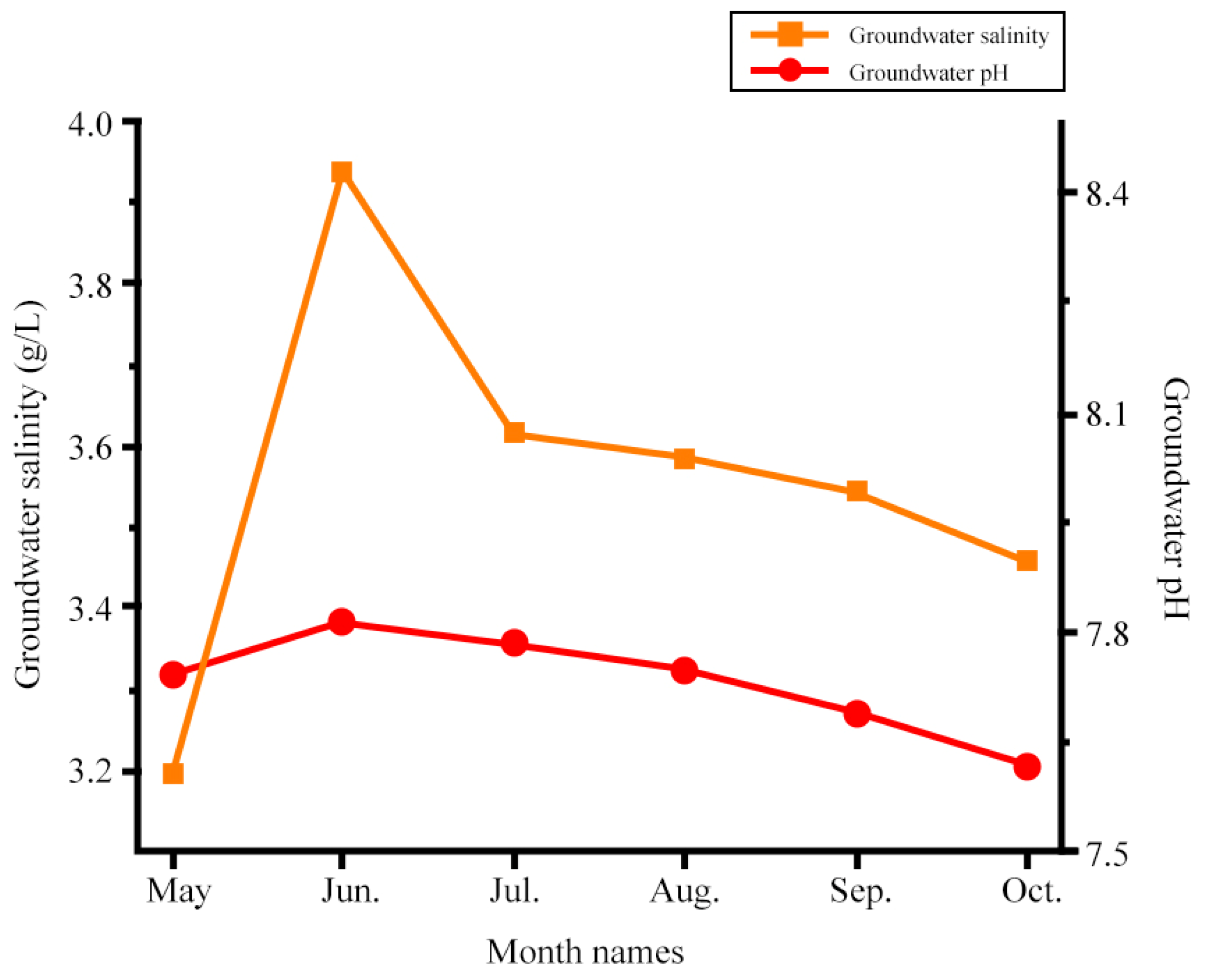
3.2.1. Temporal Changes in Groundwater Salinity and pH

Average salinity and pH data from the 2021 spring irrigation and growth periods were plotted to analyze groundwater salinity and pH variations during crop growth after improvement (Figure 4).

Groundwater salinity fluctuated between 3.19 and 3.97 g/L. During post-spring irrigation in mid-May, salinity increased due to soil salt leaching, peaking by June’s sowing period. During crop growth, plant root absorption and capillary water evaporation caused surface salt accumulation (“salt return”), resulting in a gradual decline in salinity. Groundwater pH followed similar trends with smaller fluctuations (7.82–7.61).

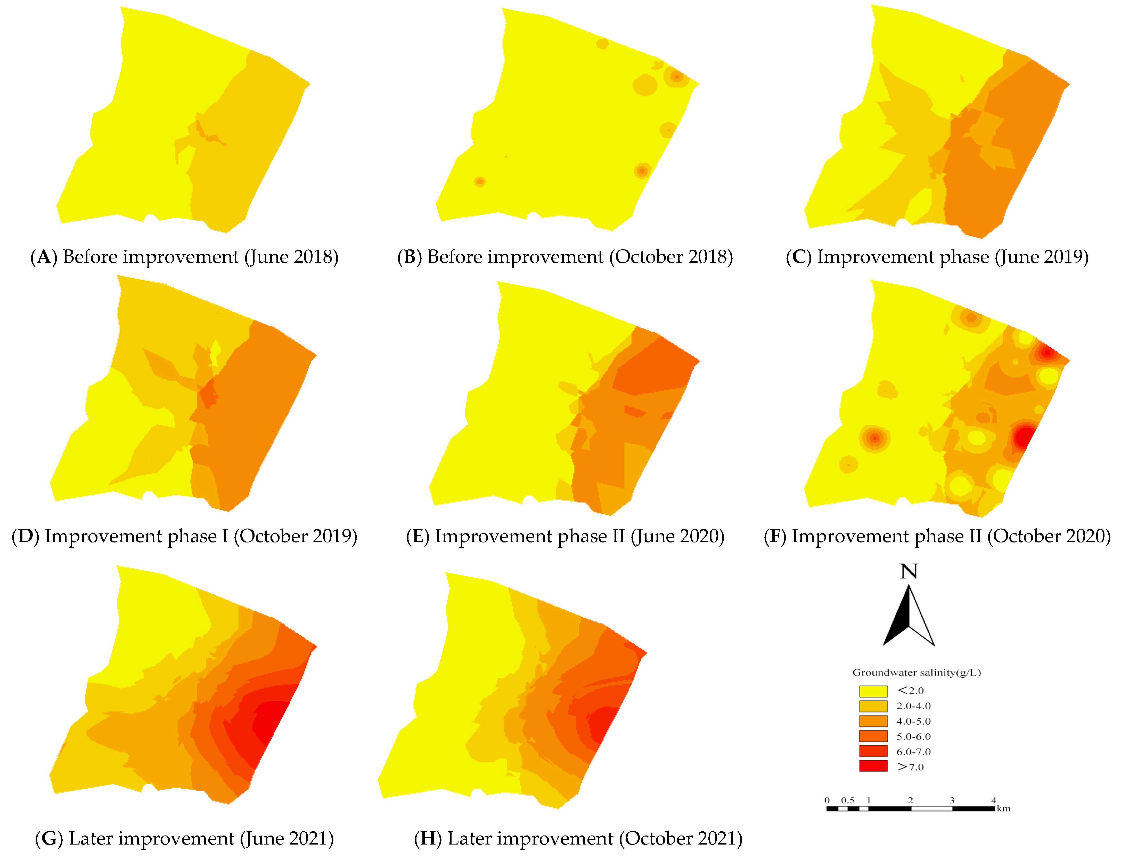
3.2.2. Spatial Distribution Characteristics of Groundwater Mineralization

This study examined how soil improvement affects the distribution of groundwater salinity. Kriging interpolation was used to analyze data from 30 observation wells. Groundwater was sampled before crop growth (June) and post-harvest (October), and spatial maps were created (Figure 5). The study area exhibits a typical saddle morphology with central north–south uplift and east–west depression, featuring secondary depressions in all quadrants. The east–west hydrological system comprises three tributaries: both the Rongfeng Branch Gully and the Sanman Sub-branch Gully, as well as the Nan Niuji Sub-branch Gully, which drain into Yitong Drainage and the Tianlai Lake, respectively. The results revealed significant west–east salinity gradients (p < 0.05), consistent with the seasonal movement patterns of high-salinity irrigation water and groundwater flow after spring irrigation, thus confirming the reliability of the field data.

Table S2 indicates that groundwater mineralization increased by 0.59, 0.80, and 1.20 g/L during the early, mid-, and late stages post-improvement (27.3–55.6% growth), demonstrating enhanced salinity leaching (p < 0.01). A high-mineralization zone (>3.5 g/L) emerged around eastern Yitong’s drainage system in the mid-late stages, occupying 18.7% of the study area. Engineering upgrades improved open ditch drainage efficiency by 32.6%, effectively facilitating lateral salt discharge.

3.3. Graphical Analysis of Groundwater Ion Sources

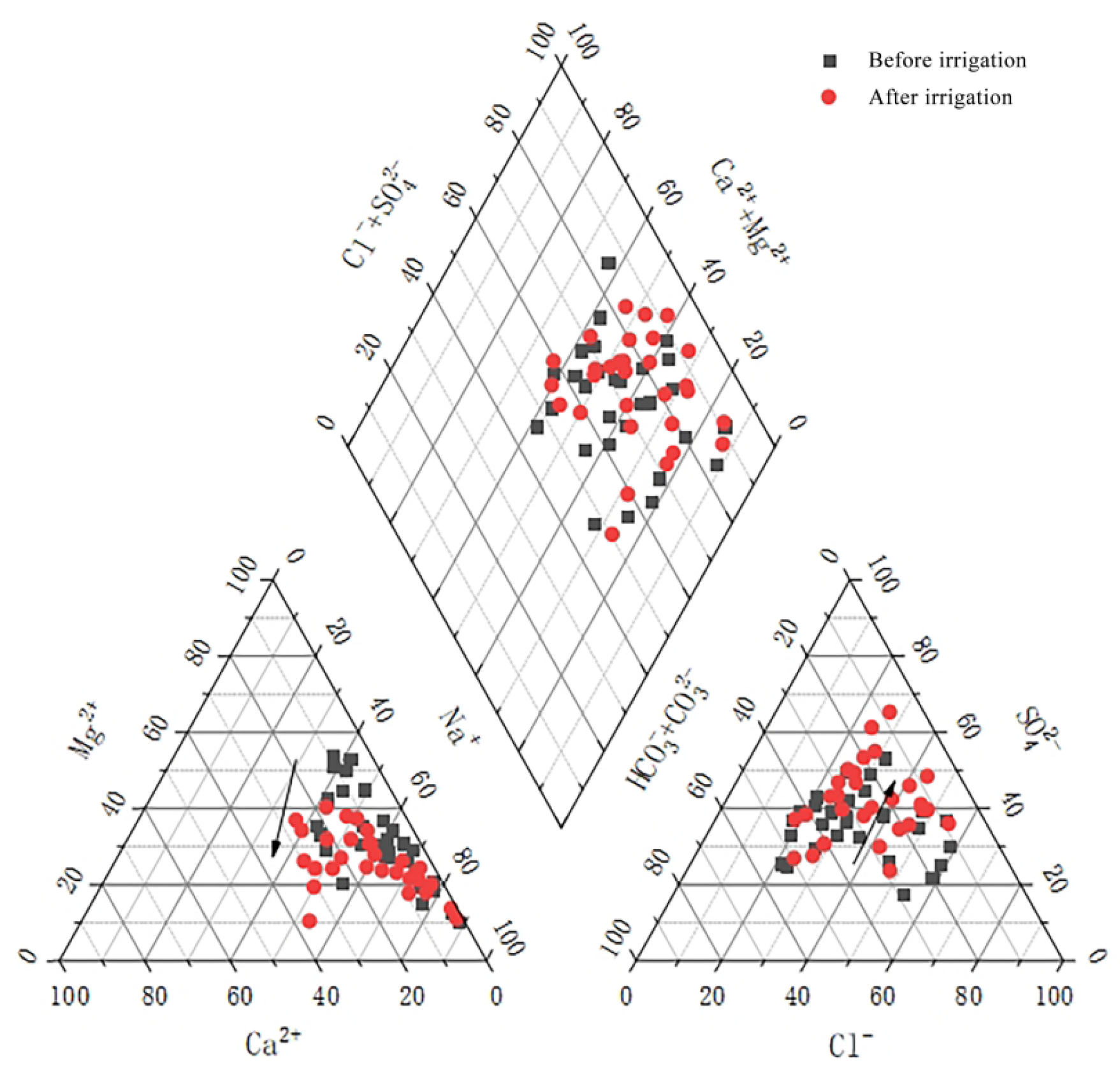
The analysis of groundwater chemistry type is vital for revealing hydrogeological and geochemical components [37]. The Piper diagram is a key hydrochemical analysis tool for visualizing water composition. This graphical tool features two triangular plots flanking a central diamond. The left triangle plots cation proportions while the right displays anion ratios. The central diamond synthesizes these ionic relationships through proportional coordinates, enabling efficient sample comparison and hydrochemical characterization. Figure 6 reveals that cations concentrate in Na+ zones (>50% milliequivalents), while anions cluster in HCO₃⁻·Cl⁻·SO₄²⁻ zones. Post-irrigation groundwater shows a decrease in Mg²⁺, a slight increase in Ca²⁺, a decline in HCO₃⁻ + CO₃²⁻, and a rise in SO₄²⁻, with stable Cl⁻ levels. The chemical types shift from Na-Mg-Cl-SO₄-HCO₃/Na-Cl-SO₄-HCO₃ to Na-Cl-SO₄.

The Gibbs diagram classifies groundwater control factors into three types using TDS vs. Na⁺/(Na⁺ + Ca²⁺) and Cl⁻/(Cl⁻ + HCO₃⁻) ratios: rainfall, rock weathering, and evaporation. With anion ratios of 0.197–0.785, groundwater samples fall between rock weathering and evaporation zones, showing these to be primary influences. The cation ratios (0.619–0.985) reveal that all Na⁺/(Na⁺ + Ca²⁺) samples exceed 0.6, with some exceeding Gibbs classification limits, indicating abnormally high Na⁺ versus low Ca²⁺ levels. Water percolation through sodium-rich soil layers increases groundwater Na⁺ concentrations during spring irrigation. The mechanism requires further analysis through chemical ion reaction theory.

The Na⁺-Cl⁻ relationship helps determine the mechanisms of salt intrusion. Figure 7 shows post-spring irrigation water samples exceeding the 1:1 line, indicating higher Na⁺ + K⁺ than Cl⁻ concentrations. This reveals that the groundwater chemistry in the study area is influenced not only by evaporated salt/silicate rock dissolution but also by cation exchange processes, explaining the elevated Na⁺ + K⁺ levels relative to Cl⁻.

Cation exchange refers to the process where under certain conditions, rock or soil particles adsorb certain cations from groundwater, thereby converting some of the original cations into components of the groundwater. The ratio γ(Na⁺ + K⁺-Cl⁻)/γ[(Ca² + Mg²⁺) − (SO₄²⁻ + HCO₃⁻)] can reflect the intensity of cation exchange. The following formula is derived from the linear regression analysis of γ(Na⁺ + K⁺-Cl⁻) and γ[(Ca² + Mg²⁺) − (SO₄²⁻ + HCO₃⁻)]:

y = −1.277x − 2.730, R² = 0.942

(1)

In the formula, y = γ[(Ca² + Mg²⁺) − (SO₄²⁻ + HCO₃⁻)], mEq·L⁻¹; x = γ(Na⁺ + K⁺-Cl⁻), mEq·L⁻¹.

γ(Na⁺ + K⁺-Cl⁻) and γ[(Ca²⁺ + Mg²⁺) − (SO₄²⁻ + HCO₃⁻)] showed a strong negative correlation, indicating that a large amount of Na⁺ in the soil layer migrated into the groundwater and exchanged cations with Ca²⁺and Mg²⁺ in groundwater after spring irrigation, resulting in a large increase in Na⁺ in water.

Spring irrigation increased the average groundwater SO₄²⁻ and Ca²⁺ concentrations by 190.45 mg/L and 38.96 mg/L, respectively, representing increases of 36.43% and 69.38%, respectively. These increases could be caused by carbonate rock weathering, evaporative shale dissolution, and water-soluble desulfurization gypsum amendments in irrigated fields.

Figure 8B shows γ(Ca²⁺ + Mg²⁺)/γ(SO₄²⁻ + HCO₃⁻) ratios below the 1:1 line, indicating higher γ(SO₄²⁻ + HCO₃⁻) levels. Post-irrigation water samples with pH > 7.4 and TDS > 600 mg/L promote CaCO₃ precipitation from Ca²⁺ and HCO₃⁻.

3.4. Hydrogeological Conceptual Model

The conditions for groundwater occurrence are complex and variable and are influenced by diverse factors [38]. This study established an accurate hydrogeological conceptual model using Visual MODFLOW software with data collected from the research area. A finite difference-based mathematical model was developed and validated, providing a foundation for future applications.

3.4.1. Scope of the Simulation Area

The simulated area spans 3.66 × 10⁷ m² in Longxingchang Town, encompassing the villages of Yifeng, Rongyi, and Yingfeng. Its boundaries were manually delineated on a calibrated satellite map. The area covers 50 km², spanning approximately 6 km east–west and 9 km north–south. See Figure S3 for details.

3.4.2. Generalization of Aquifer Conditions

The study area lies on the eastern Hetao Sag Basin’s alluvial–lacustrine plain and is divided into two aquifer groups. The first group contains alluvial–lacustrine groundwater above corresponding layers, featuring stable 50–90 m thick fine-grained lacustrine sand. The second comprises paleogeography-controlled pressurized lacustrine water with shallow upper aquifer connections.

The simulation focuses on aquifers separated by a weak permeable basal layer, which is treated as a hydraulic barrier. The shallow aquifer exhibits coarse lithology, thick stable distribution, and strong rechargeability. Its upper section contains medium-fine yellow sand, while the lower portion consists of yellow-green fine sand with a loose structure and intermittent lens-shaped cohesive layers. This aquifer is typically overlain by 3–10 m cohesive sand, displaying slight confinement. Strong hydraulic connectivity between the upper and lower sections forms a unified system that is generally treated as two heterogeneous isotropic free-flow aquifers—a 10 m cohesive sand layer and a 60 m lacustrine fine sand layer—totaling 70 m thickness with unified water levels.

3.4.3. Generalization of Boundary Conditions in the Simulation Area

(1)

Lateral boundary generalization

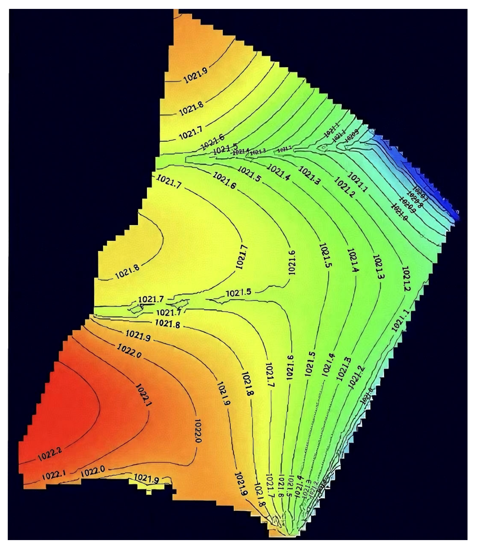
The eastern boundary of the simulation area is Yitong Drainage (generalized as a river boundary). Its southern boundary comprises Nan Niu Jia Branch Ditch (western half, river boundary) and Tianlai Lake (eastern half). This section has a fixed water level boundary, with the study area’s water level recorders showing a stable annual water level of −2.2 m for Tianlai Lake. Figure 9 illustrates the groundwater flow field from January 2020, revealing the intersecting water table lines in the study area’s western/northern boundaries. The minimal hydraulic gradient causes negligible water exchange, justifying their generalization as zero-flow boundaries.

(2)

Vertical boundary generalization

The top of the simulation area is the diving boundary, with the main replenishment sources being atmospheric rainfall, channel leakage, and irrigation backflow. Discharge occurs via diving evaporation and drainage ditch outflow. The base consists of a weak permeable layer above pressurized water, exhibiting limited hydraulic connectivity that functions as a water barrier boundary.

3.4.4. Generalization of Hydraulic Characteristics

In the simulated area, groundwater flows slowly with a natural hydraulic gradient of 1.43 × 10⁻⁴ to 3.3 × 10⁻⁴. The movement exhibits laminar flow characteristics governed by Darcy’s law. Groundwater dynamics can be generalized as a three-dimensional heterogeneous and unstable vertical anisotropic flow system due to discontinuous, thin cohesive soil layers in the shallow aquifer.

3.5. Groundwater Numerical Model

According to the conceptual model of hydrogeology in the simulation area, the groundwater numerical model is established as follows [39]:

$${\displaystyle \frac{\partial }{\partial x}}\left(\mathrm{K}{\displaystyle \frac{\partial h}{\partial x}}\right)+{\displaystyle \frac{\partial }{\partial y}}\left(\mathrm{K}{\displaystyle \frac{\partial h}{\partial y}}\right)+{\displaystyle \frac{\partial }{\partial z}}\left(\mathrm{K}{\displaystyle \frac{\partial h}{\partial z}}\right)+W=S_s{\displaystyle \frac{\partial h}{\partial t}}(x,y,z)\in \Omega$$

(2)

$$h\left(x,y,z,t\right){|}_{t=0}=h_0\left(x,y,z\right) (x,y,z)\in \Omega$$

(3)

$${\left(\mathrm{K}{\displaystyle \frac{\partial h}{\partial x}}\right)}_{\Gamma 2}=q_1\left(x,y,z,t\right) (x,y,z)\in {\Gamma }_2$$

(4)

$${\left(\mathrm{K}{\displaystyle \frac{\partial h}{\partial x}}\right)}_{\Gamma 3}={\displaystyle \frac{k_1}{m_1}} (h_n-h) (x,y,z)\in {\Gamma }_3$$

(5)

In the formula, Ω—seepage area; Γ₂, Γ₃—second and third boundaries; h—groundwater level (m); t—time (d); K—permeability coefficient (m/d); m—aquifer thickness (m); S_S—storage rate (L⁻¹); W—vertical recharge/discharge intensity (1/d); h₀—initial groundwater level (m); q₁—the second boundary’s single-width flow rate (m/d); and h_n—external groundwater level at the third boundary (m).

3.6. Establishment of the Numerical Model

The groundwater numerical model was established using Visual MODFLOW for the established hydrogeological model.

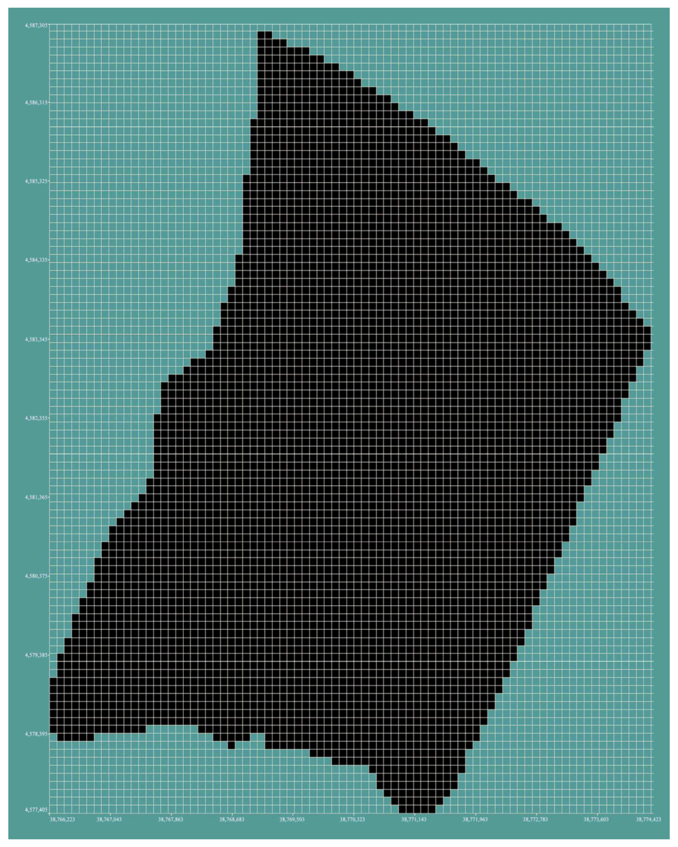
3.6.1. Grid Division of Simulation Area

(1)

Spatial dispersion

Discrete mesh refinement methods include finite difference, finite element, and non-uniform mesh approaches [40]. This simulation employed the equal-interval finite difference method, with calculations at grid centers. The 100 m × 100 m area was divided into grids (99 rows, 82 columns, and 8118 total cells), with 5312 effective cells. The results are shown in Figure 10 and Figure S4.

(2)

Time dispersion

The groundwater model’s identification period spans from 1 January to 31 December 2020, with validation performed for the period from 1 January to 31 October 2021. Both phases use monthly stress periods (12 for identification and 10 for validation), each with 10-day time steps. Initial groundwater levels were simulated using observation well data for January 2020, with the initial contour map generated through Kriging interpolation (Figure 9).

3.6.2. Hydrogeological Parameter Zoning

The simulation area is small and predominantly consists of arable land. Preliminary investigations show minimal lithological variation, allowing for its treatment as a single hydrogeological parameter zone. Quaternary strata exceeding 1000 m in thickness dominate, with Holocene (Q4) and Upper Pleistocene (Q3) aquifers. Q4 and Q3 contain clay–fine sand alternations and medium-fine sand, silt, and thin cohesive layers, respectively. Hydrogeological parameters were assigned using pumping tests, geological surveys, and reference values from GWI-D1 and the Embankment Engineering Manual. Permeability coefficients are presented in

Table 1. Aquifer permeability coefficients.

Osmotic Coefficient	Kx/(m/d)	Ky/(m/d)	Kz/(m/d)
Model layer 1	0.81	0.81	0.81
Model 2	8.2	8.2	0.82

, while other parameters are given in

Table 2. Hydrogeological parameters.

	Coefficient of Storage	Specific Yield	Total Porosity
Model layer 1	5 × 10−3	0.03	0.35
Model 2	1.5 × 10−3	0.21	0.29

.

3.6.3. Treatment of Source and Sink Items

The source–sink term quantifies water supply/discharge per unit of time in the model. For this simulation area, it is calculated separately for freeze–thaw and non-freeze–thaw periods. The non-freeze–thaw “source” includes precipitation infiltration, irrigation infiltration, and lateral runoff infiltration, while the “sink” comprises evaporation, lateral discharge, and drainage ditch outflow.

Groundwater level data are used to calculate the total water volume changes during freeze–thaw cycles by multiplying hydraulic head differences with the area’s water supply rate (μ). This total represents combined source–sink fluxes (infiltration, recharge, evaporation, and discharge). Negative fluxes (water level decline) are modeled via evapotranspiration, while positive fluxes (water level rise) are input through the Recharge module.

(1)

Rainfall infiltration recharge

Rainfall infiltrates the soil by gravity, entering the unsaturated zone to recharge groundwater. Precipitation data from the FM-QX meteorological station in the simulation area are shown in Figure S5 (annual data for 2020). Initially set at 0.3 according to the local soil type and the Technical Requirements (GWI-D1), the infiltration calculation is determined using precipitation data. This value is input via the Recharge module using the following formula:

Q = P·C·S

(6)

where

• Q—monthly rainfall infiltration recharge in the simulation area;
• P—monthly rainfall in the simulation area;
• C—infiltration coefficient of rainfall in the simulation area;
• S—area of the simulation zone.

(2)

Field irrigation infiltration recharge

Field irrigation infiltration recharge refers to the amount of water that percolates downward through the soil capillary zone after entering the farmland from the simulated area and then recharging the groundwater. Based on the groundwater depth and surface rock properties of the simulation area, the field irrigation infiltration recharge coefficient β is selected as 0.3. The calculation formula is as follows:

Q_pump = Q_field · β

(7)

where

• Q_pump—simulated field irrigation infiltration recharge;
• Q_field—simulated irrigation amount;
• β—infiltration coefficient of irrigation in the simulation area.

The infiltration recharge of field irrigation in the simulation area was input into the model through the surface Recharge module, and the range of surface recharge was determined by the improved remote sensing satellite map of the simulation area.

(3)

Canal Irrigation Infiltration Recharge

Channel seepage recharge refers to the process where water from canals is replenished by groundwater due to leakage during water conveyance. The annual irrigation water diversion in the 3.66 × 10⁷ m² project area is 25.1363 million m³. In the simulation area, the field channels and farm channels were lined with gabions. After the installation of this lining, the water use coefficients of these canals reached 0.95 and 0.96, respectively. Therefore, this simulation only calculates the channel seepage recharge of the main canals, using the following formula:

Q_s = m · Q_w = γ (1 − η) · Qy

(8)

where

• Q_s—infiltration recharge of the sublateral canal;
• m—the replenishment coefficient of the channel leakage;
• η—the water use coefficient of the furrow irrigation in the simulation area, which is 0.861;
• γ—the correction coefficient, which is 0.70 according to the Hydrogeological Exploration Report of the Hetao Irrigation District.

The irrigation infiltration recharge of the furrow channel was input into the model through the surface Recharge module, and the range of surface recharge was consistent with that of the field irrigation infiltration recharge.

(4)

Evaporation coefficient

Subsurface evaporation depends on the evaporation rate, evaporation coefficient, and maximum evaporation depth in the simulation area. Evaporation data are sourced from the area’s FM-QX meteorological station (Figure S6). The evaporation coefficient relates to subsurface lithology and groundwater depth. Monthly coefficients are determined based on annual variations in groundwater depth (Table S3). Evaporation discharge is modeled through the Evapotranspiration module.

(5)

Drainage capacity of the ditch

When the simulated area’s groundwater level exceeds the bottom elevation of the drainage ditch, groundwater discharges through the ditches as open ditch drainage. Four drainage ditches exist, namely the Nan Niuji Branch Ditch, San Man Branch Ditch, Rongfeng Sub-ditch, and Yitong Drainage. These ditches were dredged and improved as part of the soil improvement project. Their cross-sectional diagrams were used to establish design elements such as bottom elevation, width, and slope, which were input into the model via the River module.

3.7. Model Identification and Verification

The simulation area’s initial conditions, groundwater levels, source–sink terms, and well data were input into the model using 2020 data and 2021 groundwater data for model identification and validation, respectively. Simulations were run to obtain annual groundwater level calculations. These were compared with the levels measured during identification, and then hydrogeological parameters and source–sink terms were refined to fall within allowable ranges to minimize errors and ensure model accuracy.

3.7.1. Model Identification

This study identifies the model using trial algorithms by inputting initial/boundary conditions and source–sink terms. The calculated and measured water levels are compared, with the hydrogeological parameters being repeatedly adjusted until a good fit is achieved. The 2020 identification period incorporates groundwater data. Figure 11 and Figure S7 and

Table 3. Error between calculated head and observed head of groundwater in the simulation area during the identification period.

	Absolute Mean Error (m)	Standard Estimate Error (m)	Correlation R2
Sunflower field	0.21	0.02	0.89
Corn field	0.26	0.031	0.82

present the fitting plots, scatter plots, and error data for different land types during this period.

The identification results show that over 85% of wells have <0.3 m error between the measured and calculated groundwater levels, demonstrating good model alignment with monitoring data. This confirms the model’s compliance with “Technical Requirements for Numerical Simulation of Groundwater Flow” (GWI-DI) accuracy standards [41]. In cases where the water level change value is small (<5 m), the water level fitting error should generally be less than 0.5 m, validating reasonable aquifer structure assumptions, boundary conditions, and hydrogeological parameter selection. It is noteworthy that these standards apply to flat terrain with a low hydraulic gradient, such as that found in the Hetao Irrigation District.

Table 4. Aquifer permeability coefficients on the calibrated.

Osmotic Coefficient	Kx/(m/d)	Ky/(m/d)	Kz/(m/d)
Model layer 1	0.9	0.9	0.9
Model 2	8.64	8.64	0.864

and

Table 5. Hydrogeological parameters on the calibrated.

	Coefficient of Storage	Specific Yield	Total Porosity
Model layer 1	5.2 × 10−3	0.02	0.42
Model 2	1.5 × 10−3	0.25	0.33

provide statistical data on the calibrated hydrogeological parameters.

3.7.2. Model Verification

The model’s reliability was verified using January–October 2021 data from the simulation area. The hydrogeological parameters and boundary conditions of the identified model were not changed. The groundwater depth in 2021, as well as the test data, atmospheric precipitation infiltration recharge, field irrigation infiltration recharge, canal irrigation leakage recharge, lateral runoff recharge, vertical evaporation, and drainage ditch discharge, were all input into the model for calibration. Figure 12 and Figure S8 display comparative and scatter plots of calculated versus measured well water levels across the land categories during validation.

Table 6. Errors between the calculated head and observed head of groundwater in the simulation area during the verification period.

	Absolute Mean Error (m)	Standard Estimated Error (m)	Correlation R2
Sunflower field	0.14	0.015	0.95
Corn field	0.24	0.054	0.92

presents the groundwater head calculation errors during this period.

During model validation, over 85% of the wells showed measured vs. calculated groundwater level errors under 0.3 m, indicating a good level of model accuracy meeting GWI-DI standards. This confirms that the adjusted aquifer structure, boundary conditions, and hydrogeological parameters properly represent the area’s groundwater flow dynamics.

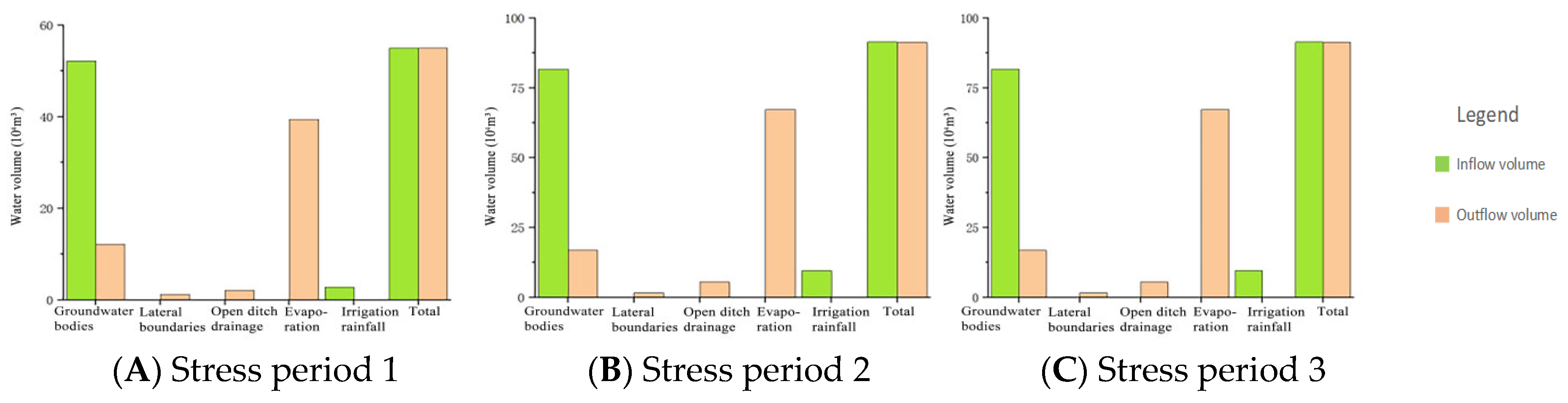
3.8. Groundwater Balance in the Simulation Area

Groundwater equilibrium describes the balance between groundwater recharge and discharge regarding water volume, solute content, and heat within specific spatiotemporal parameters [42]. It manifests in equilibrium (recharge equals discharge), negative equilibrium (recharge < discharge), and positive equilibrium (recharge > discharge) states. In this study, groundwater equilibrium is calculated separately for the identification and validation periods within the simulation area using a water balance equation.

A − B = ∆V

(9)

In the formula, A represents the following equilibrium area input items: atmospheric rainfall X, surface water inflow Y₁ (channel leakage, field irrigation infiltration), lateral inflow Z₁ at fixed head boundary, and groundwater inflow W₁ (negligible water condensation). B denotes the following output items: surface water outflow Y₂ (open ditch drainage), lateral outflow Z₂ at the fixed head boundary, and groundwater outflow W₂.

∆V and μ∆H represent the change in volume during the equilibrium period and the groundwater level amplitude (where H is multiplied by the water supply degree μ of the aquifer), respectively. The final expression of the water balance equation is as follows:

(X + Y₁ + Z₁ + W₁) − (Y₂ + Z₂ + W₂) = μ∆H

(10)

The results of the equilibrium relationship between each stress period and the annual equilibrium water quantity during the verification period calculated using Visual MODFLOW software are shown in Figure 13 and Figure 14 and the Supplementary Materials, Figure S9 and Figure S10, and Table S4, respectively.

Stress period 1–2 (freezing–thawing): Surface frost layer thickening causes negative groundwater equilibrium through runoff discharge and permafrost storage, lowering water levels. Stress period 3–4 (thawing): Frozen layer meltwater splits into matrix infiltration recharge and surface runoff. Increasing subsurface evaporation leads to a water surplus, elevating levels under the dominance of freezing–thawing infiltration. Stress period 5–6 (spring irrigation): Agricultural irrigation raises the groundwater, boosting channel discharge and evaporation through irrigation–recharge–discharge synergy. Stress period 7–9 (crop growth): Reduced irrigation/precipitation infiltration and peak evaporation return groundwater to a low level, with this decline governed by evaporation–runoff coupling. Stress period 10–11 (autumn irrigation): The resumption of irrigation during autumn raises groundwater again, notably increasing channel discharge under irrigation-driven positive recharge. Stress period 12 (initial freezing): Surface ice inhibits evaporation while the development of the frozen layer slows discharge, stabilizing water fluctuations. These dynamics reveal annual cyclical groundwater evolution patterns.

The water balance diagram lists components sequentially as follows: groundwater runoff, lateral exchange at fixed head boundaries, open channel discharge, subsurface evaporation, surface recharge (precipitation infiltration, channel leakage, and irrigation backflow), and total balance.

The study area exhibits a minor negative water balance during both the identification (absolute difference 0.039 × 10⁴ m³) and verification periods (0.041 × 10⁴ m³), linked to the declining groundwater levels, though the model errors remain acceptable. Infiltration recharge (<5% annual) and lateral exchange (<3% annual) minimally affect water balance due to (1) the arid climate with 182 mm annual precipitation vs. 8.2× higher evaporation and (2) the flat terrain (<0.5‰ slope), low hydraulic gradient (≤0.15 m head difference), and impermeable surface sediments (K = 1.2 × 10⁻⁶ m/s), which limit lateral flow. Irrigation leakage plays the dominant role in recharge (66.99% identification; 55.67% verification), while discharge primarily occurs through channel drainage (26.95–26.31%) and subsurface evaporation (31.99–47.09%), highlighting agricultural drainage efficiency and evaporation as key groundwater regulators.

3.9. Prediction of the Groundwater Level in the Simulation Area

3.9.1. Establishment of the Forecasting Model

• Time discretization and initial flow field setting

This study establishes a 10-year water level forecast (January 2021–December 2031) with non-uniform time intervals, dividing the period into 120 stress periods of 30 days each and 10-day time steps. The initial flow field uses actual groundwater well data from January 2021 in the study area. Kriging-generated groundwater contour maps serve as the numerical model’s initial head field.

2.

Boundary condition prediction and parameterization

Proper boundary condition settings crucially influence the accuracy of groundwater simulations. This study dynamically adjusts the original model boundaries in the following ways: (1) it retains zero-flux boundaries at the western (S212 Road) and northern (National Highway 110) edges; (2) it maintains river boundaries for eastern Yitong Drainage (Type 3 boundary), with an annual drainage coefficient reduction of 2%, considering sedimentation; and (3) it implements a hybrid southern treatment–river boundary for Nan Niuji Branch and a constant–head boundary near Tianlai Lake (Type 1), both featuring an annual drainage coefficient decrease of 2%.

3.

Spatiotemporal prediction of meteorological elements

Using Wuyuan County’s rainfall data (1981–2010), a fuzzy Markov chain was used to predict rainfall for the next decade. The annual rainfall ranged from 56.3 mm to 267.6 mm during this 30-year period, showing high randomness. The calculated average was 176.4 mm with a 55.14 mm standard deviation. A five-level rainfall classification was created via the mean–standard deviation method:

Class I (drought year): P < μ − 1.1σ (<115.75 mm);

Class II (dry year): μ − 1.1σ ≤ P < μ − 0.5σ (115.75–148.83 mm);

Class III (normal year): μ − 0.5σ ≤ P < μ + 0.5σ (148.83–203.97 mm);

Class IV (favorable year): μ + 0.5σ ≤ P < μ + 1.1σ (203.97–237.05 mm);

Class V (flood year): P ≥ μ + 1.1σ (≥237.05 mm).

The autocorrelation coefficient (r_k) and transfer probability matrix are calculated based on this system, and the 2021–2030 rainfall prediction range and Hurst index are determined via fuzzy set theory. The results are shown in Figure 15.

4.

Irrigation amount and human factors

The study area’s irrigation system and crop types remained consistent annually; thus, their changes in the prediction model aligned with the model’s identification and verification period. Since no artificial groundwater extraction or water facilities impacted groundwater levels, these human factors were excluded [43,44].

3.9.2. Model Prediction Results

The initial flow field of groundwater, established boundary conditions, and source and sink terms were input into the corresponding modules of the model to obtain the prediction results for the next 10 years, as shown in Figure 16 and the Supplementary Materials, Figures S11 and S12.

The predicted groundwater flow field shows higher levels in the southwest of the study area, with overall west-to-east flow consistent with actual conditions. Figure 17 indicates a gradual 10-year decline in average groundwater levels, primarily influenced by irrigation patterns. This suggests that groundwater levels will remain stable at post-saline–alkali improvement stages under current irrigation systems and crop structures.

3.10. Changes in Groundwater Level Under Different Irrigation Scenarios

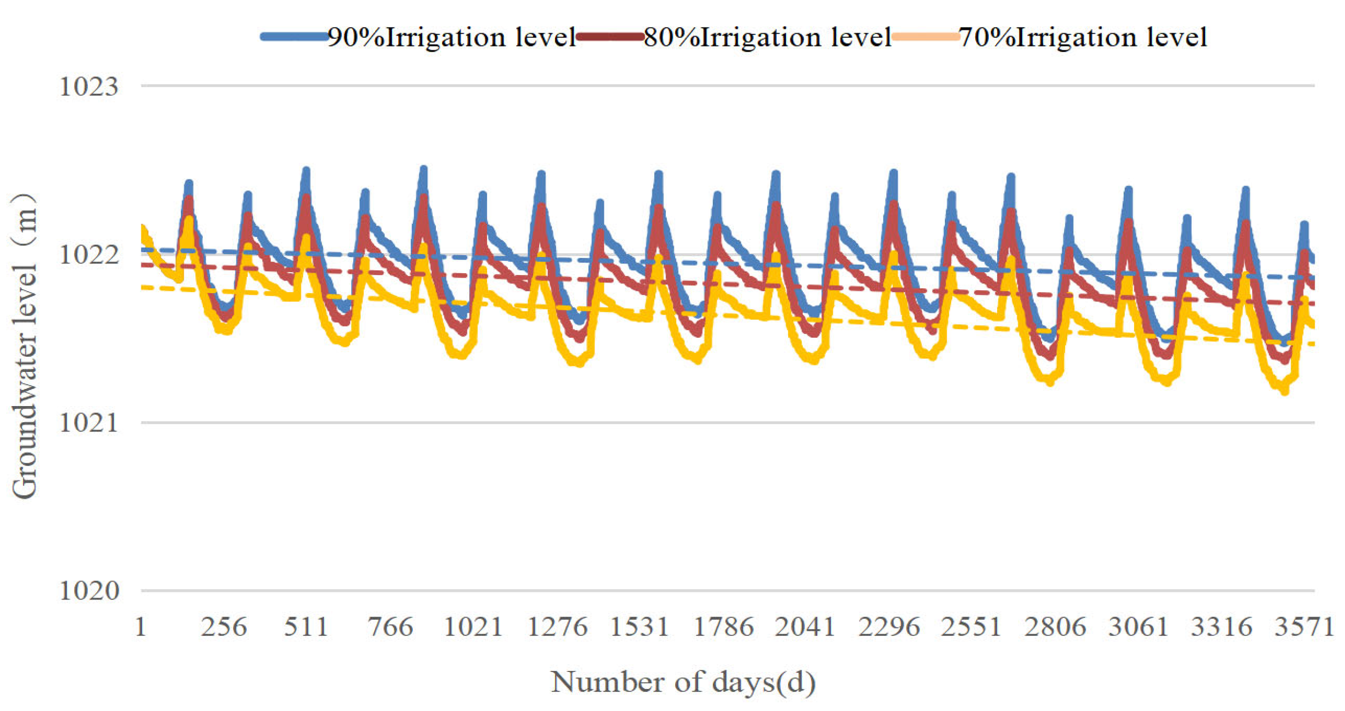
Previous studies indicate that the study area’s shallow groundwater levels during early crop growth (June–August) reduce water efficiency and increase salinization risks. With mandatory water-saving measures in the Hetao Irrigation District decreasing annual Yellow River irrigation, this study focuses on irrigation (the primary groundwater depth factor) by modeling three reduced irrigation scenarios. The model used 90%, 80%, and 70% of normal irrigation volumes, with corresponding parameters input to predict decade-long groundwater level changes, as shown in Figure 18 and

Table 7. Characteristics of groundwater level at different irrigation levels.

Irrigation Volume	Maximum Groundwater Level	Minimum Groundwater Level	Average Groundwater Level
Normal irrigation levels	1022.946	1021.462	1022.106
90% irrigation level	1022.508	1021.469	1021.941
80% irrigation level	1022.338	1021.362	1021.819
70% irrigation level	1022.208	1021.177	1021.633

.

As shown in Figure 18, there were variable declines in groundwater levels under the three different irrigation levels. The annual decrease was smaller at 90% and 80% irrigation, with 0.165 m and 0.287 m drops over the span of a decade, but greater at 70% irrigation, with a 0.473 m drop (Table 7). Groundwater is sensitive to changes in irrigation levels, particularly at the maximum levels. The minimum irrigation levels in March are mainly influenced by soil freezing. Using 80% irrigation effectively reduces water usage from the Yellow River while controlling groundwater depth, thus improving water efficiency and reducing salt stress.

4. Discussion

4.1. The Alterations in the Physical and Chemical Characteristics of Groundwater

The hydrochemical properties of groundwater serve as a comprehensive indicator of environmental variations within aquifer systems. Concurrently, identifying the provenance of dissolved constituents in groundwater constitutes a critical component in assessing both groundwater resource sustainability and hydrogeochemical environmental quality [45,46]. Yuan et al. [47] conducted a comprehensive analysis of the temporal variations in nitrogen–phosphorus concentrations and hydrochemical characteristics within the Wulate Irrigation District during pre- and post-autumn irrigation periods. Their findings revealed that groundwater chemistry exhibited dual control from evaporation–concentration effects and anthropogenic influences, with anions demonstrating particular susceptibility to agricultural activities, similar to the results of this study. Hou et al. [48] performed an in-depth examination of autumn irrigation impacts on groundwater hydrochemistry within the Yichang Irrigation District. The study established that autumn irrigation operations significantly enhanced soil salinity leaching efficiency, with optimized post-irrigation groundwater drainage intensity proving crucial for improving regional desalination effectiveness; similar conclusions were also drawn in this study. To elucidate the formation mechanisms of shallow groundwater in the Fengpei Plain, Zhu et al. [49] implemented a systematic hydrogeochemical investigation. Their methodology encompassed the collection of 27 representative shallow groundwater samples, followed by the application of multivariate analytical techniques including classical statistical analysis, Sukharev classification, Gibbs diagrams, and ionic ratio analysis. This integrated approach enabled the comprehensive characterization of hydrochemical properties and evolutionary processes in the study area’s shallow aquifer system.

Through the systematic monitoring of hydrogeological parameters, this study reveals a progressive decline in groundwater elevation within the study area concomitant with the advancement of soil improvement measures. The groundwater table demonstrated a sustained downward trajectory, culminating in post-treatment annual mean water table depths ranging from 1.589 to 1.686 m, with stabilization also being observed at approximately 1.63 m. A comparative analysis with pre-treatment hydrological conditions indicated a marked reduction in groundwater elevation following geotechnical interventions. Hydrological budget quantification identified precipitation as having minimal influence on aquifer dynamics (R² = 0.12), whereas Yellow River irrigation inputs and evaporative flux demonstrated more pronounced effects on groundwater depletion patterns (p < 0.05).

Post-improvement analysis shows an extreme mineralization zone (4.2–4.8 g/L) in the groundwater, located in transitional zones where gentle slope diffusion aligns with topography-driven salt enrichment (R² = 0.87). The region’s low hydraulic gradient (0.12) prolongs groundwater retention (47–62 days), thus increasing the salinization risk index and the probability of secondary soil salinization to 0.78 (critical 0.65) and 31.4% ± 3.2%, respectively.

The research shows that soil improvement boosts irrigation efficiency (19.8%) and drainage performance (28.4%), regulating west–east groundwater salinity migration. However, the micro-morphology of the central-eastern lowland has created a geochemical salt barrier, thus increasing groundwater mineralization above ecological safety thresholds (3.0 g/L). This necessitates targeted vertical well discharge or biological desalination for risk management.

The predominant cation and anion in the groundwater of the study area are Na⁺ and HCO₃⁻·Cl⁻·SO₄²⁻, respectively. Post-irrigation groundwater shows a decrease, slight increase, decline, and rise in Mg²⁺, Ca²⁺, HCO₃⁻ + CO₃²⁻, and SO₄²⁻, respectively, with stable Cl⁻ levels. Spring irrigation increased groundwater total dissolved solids by 15.6% on average. Water chemistry evolves through rock weathering, evaporation, and cation exchange. The dominant chemicals are Na-Mg-Cl-SO₄-HCO₃ and Na-Cl-SO₄-HCO₃, with Cl- and K⁺⁺Na⁺ being the primary ions (averaging 482 mg/L and 356 mg/L). With variation coefficients >0.65, these ions demonstrate marked spatial variability and serve as critical indicators of groundwater salinization.

The efficiency of soil salt leaching declines exponentially with depth. The heterogeneous hydraulic conductivity characteristics among stratigraphic units, attributable to differential irrigation volumes and textural composition variations, resulted in a 10–20 day phreatic response period for aquifer systems throughout the study area in order to attain peak water table elevation following spring irrigation initiation. Hydrometric monitoring revealed a pre- and post-irrigation groundwater fluctuation amplitude of 1.197–2.142 m, corresponding to mean daily recharge rates of 0.0798–0.169 m/d. Post-irrigation soil analysis demonstrated significant reductions in electrical conductivity (EC) throughout the 0–100 cm profile, with maximum salt-leaching efficacy observed in the surficial horizon (0–20 cm). This epipedon exhibited a mean salinity reduction of 47.11%, indicating superior desalinization performance in surface soils. Subsurface analysis revealed the depth-dependent attenuation of leaching effects; as the soil depth increased, the desalination effect of the soil gradually decreased, demonstrating an inhibitory effect of reduced soil permeability on solute transport.

4.2. Advantages of Applying Numerical Groundwater Models

Fiorese et al. [50] used an integrated SWAT-MODFLOW approach to successfully address the challenges posed by the distinctive characteristics of karst systems in Salento (Italy). Additionally, the incorporation of satellite data enhances the precision and dependability of the model by augmenting the traditional datasets. Yang Yang et al. [51] employed the Visual MODFLOW numerical model to investigate the spatiotemporal dynamics of groundwater systems in the Hetao Irrigation District under the conjunctive utilization of well–canal irrigation. The simulation results demonstrated that implementing the well–canal conjunctive irrigation scheme induced a notable increase in groundwater table depth across the entire irrigation region; however, distinct spatial heterogeneity manifested in groundwater depth variations among the different irrigation subzones. Lu Xiaoli et al. [52] employed the GMS numerical modeling platform to develop a coupled groundwater seepage and solute transport model for the experimental site. The researchers formulated three distinct groundwater resource exploitation and management scenarios, conducting numerical simulations to evaluate hydrogeological recovery efficiency and assess saline intrusion mitigation performance along the southern boundary. Although a series of water–salt models at the field scale has been established both domestically and internationally, these models fail to fully account for the complex spatial variability of multiple factors such as meteorology, hydrogeology, soil, irrigation, and crops. This poses certain challenges for groundwater research at the regional scale. Especially in areas where cultivated and non-cultivated land alternate and where soil salinization varies over time and space, the implementation of large-scale soil salinity and alkalinity improvement projects has led to significant changes in the water cycle and groundwater depth in the irrigation areas.

The groundwater numerical simulation imposes rigorous constraints on the boundary conditions and hydrogeological parameters of the study area while posing substantial challenges in parameter acquisition. Furthermore, the improper delineation of hydrogeologic boundaries and aquifer configurations frequently results in diminished predictive accuracy and model inaccuracies [53,54]. Consequently, it is imperative to develop a high-fidelity groundwater conceptual model through the integration of reliable hydrogeological parameters and well-constrained boundary conditions prior to conducting numerical simulations. Subsequent validation against empirical groundwater observational data enables the establishment of an authentic groundwater numerical model.

This study established an accurate hydrogeological conceptual model using Visual MODFLOW software with data collected from the research area. And a finite difference-based mathematical model was developed and validated. During model validation, over 85% of wells display <0.3 m error between the measured and calculated groundwater levels, demonstrating good model alignment with monitoring data. This confirms the model’s compliance with GWI-DI accuracy standards, validating reasonable aquifer structure assumptions, boundary conditions, and hydrogeological parameter selection. However, due to the relatively short current observation period (2018–2021), conducting a ten-year-scale data simulation under the condition of limited observational data will introduce certain errors and limitations. Short-term data may miss extreme events, periodic changes, or long-term trends, leading to simulation deviations. At the same time, uncertainties such as input errors and model structure flaws will be significantly amplified through positive feedback in long-term simulations. Considering that the primary focus of our modeling approach and model parameterization is on studying the spatiotemporal evolution laws and influencing factors of the groundwater environment under the background of soil salinization and alkalization improvement projects, some dataset limitations warrant acknowledgment. It is planned to gradually correct the prediction deviations by continuously conducting grid monitoring and using high-precision satellite data in the future.

The groundwater system in the study area exhibits a persistent negative equilibrium regime. Quantitative analysis reveals that channel infiltration and irrigation return flow constitute the predominant recharge components, accounting for 66.99% and 55.67% of total recharge during both the model calibration and validation periods, respectively. Regarding discharge mechanisms, open ditch drainage and phreatic evaporation emerge as the primary discharge components, with respective contributions of 26.95% versus 26.31% for drainage and 31.99% versus 47.09% for evaporation across calibration and validation phases.

Through the parameterization of regional boundary conditions and meteorological forces, a decadal-scale groundwater prediction model was developed, which demonstrated spatiotemporal consistency to observed system behavior. The simulation results indicate a marginally decreasing trend in mean groundwater levels over the 10-year projection period. Hydraulic fluctuation analysis demonstrates that irrigation return flow serves as the principal modulator of water table dynamics. Under current irrigation practices and crop rotation patterns, model projections suggest the eventual stabilization of aquifer levels at post-salinization remediation baselines.

The scenario analysis of irrigation reduction strategies (90%, 80%, and baseline water applications) reveals progressive groundwater decline across all cases. Notably, the 90% and 80% irrigation scenarios achieve new dynamic equilibria within the simulation timeframe. The integrated analysis of groundwater drawdown characteristics indicates that implementing 80% irrigation quotas achieves the following dual objectives: (1) a substantial reduction (20%) in surface water diversion demands can better meet the requirements of China’s Yellow River water allocation schemes, and (2) the maintenance of optimal groundwater depths (1.8–2.2 m) for the concurrent enhancement of crop water use efficiency (12–15% improvement projected) and mitigation of soil salinization stress.

The Hetao Irrigation District primarily depends on Yellow River diversions for agricultural water supply, facing a critical challenge where peak crop water demand mismatches scheduled irrigation periods. To compensate, groundwater extraction supplements surface water shortages during dry intervals. Recent monitoring shows sustained groundwater depletion, reducing aquifer sustainability and intensifying reliance on river diversions, thereby destabilizing regional water management. This cyclical pattern threatens sustainable agricultural water security. Simultaneously, traditional flood irrigation causes dual environmental effects: carbonate/sulfate accumulation from river water induces soil salinization, while cyclical groundwater fluctuations drive salt redistribution through infiltration–evaporation processes, accelerating topsoil salt accumulation. By adjusting the water resource allocation plan, not only can the water demand be alleviated, but also the pressure of soil salinization can be relieved. This will further promote the high-quality development of agriculture and is of great significance for alleviating the water use contradiction between upstream and downstream in the Yellow River Basin, supporting regional economic development, ensuring national food security, and maintaining stability in the border areas. Therefore, the Hetao Irrigation District should actively adapt to water resource constraints and explore ways to accelerate the high-quality development of agriculture under the existing water resource constraints.

4.3. Prospects

This study examined the hydrogeological impacts of soil improvement via multi-source data fusion and established an irrigation area-scale groundwater model. In future designs, breakthroughs can be sought in the following aspects:

(1)

Due to the simplistic field irrigation management approach, there will inevitably be deviations in the irrigation quotas for each plot, which will lead to the inaccurate input of the Recharge module in the groundwater numerical model’s source–sink terms, thereby affecting the model’s accuracy. Therefore, in the subsequent application of the model, it is necessary to conduct more detailed investigations of the actual situation in the study area in the first place. Secondly, increasing the monitoring of the irrigation water volume for each plot can enhance the simulation accuracy of the model. Thirdly, on-site verification should be conducted to make adjustments after the simulation, which can further reduce the model error.

(2)

The absence of comprehensive monitoring data hinders the precise assessment of quantitative effects stemming from irrigation reduction in the groundwater balance. Future research endeavors should integrate long-term observational datasets with advanced isotope tracing techniques to elucidate the mechanisms governing water–salt transport dynamics under diverse irrigation management strategies. Furthermore, systematic investigation into machine learning algorithms and hybrid modeling frameworks could substantially enhance predictive accuracy in hydrological simulations.

5. Conclusions

This study analyzes groundwater monitoring data, soil parameters, and hydrogeological surveys from both before and after soil improvement projects. It reveals a spatiotemporal evolution of groundwater depth, salinity dynamics, and water quality change mechanisms in saline–alkali land remediation. The research quantifies the impact of irrigation on ion migration and soil salt redistribution in groundwater. The 3D Visual MODFLOW groundwater model developed in this study enables balanced quantitative analysis and predictive simulations of groundwater levels under different irrigation scenarios, providing scientific support for evaluating the environmental effects of the Hetao Irrigation District’s land management project. The main conclusions are as follows:

(1)

Following soil improvement projects, groundwater depth in the study area significantly declined, stabilizing at an average annual depth of 1.63 ± 0.15 m (0.40 m lower than pre-improvement). The measures enhanced irrigation leaching and open ditch salt discharge, causing increases in phased salinity. During the early, mid, and late stages of the project, salinity rose by 0.59 g/L, 0.80 g/L, and 1.20 g/L, respectively, from the baseline. This demonstrates significant lag effects in soil–groundwater salt migration.

(2)

Groundwater equilibrium calculations indicate that the study area is in negative equilibrium. Recharge components show channel seepage and irrigation recharge contributions of 66.99% (rate period) and 55.67% (verification period), respectively. Discharge components are dominated by open ditch drainage (26.95–26.31%) and groundwater evaporation (31.99–47.09%), highlighting the regulatory role of artificial drainage systems in groundwater circulation.

(3)

Numerical simulations indicate that maintaining current irrigation systems and planting structures could stabilize groundwater levels at 1.60–1.65 m over the next decade, thus confirming the sustainable hydrological effects of soil improvement measures. Reducing irrigation to 80% of the current water supply of the Yellow River enables groundwater level stabilization (2.05 ± 0.12 m burial depth) within 5–7 years. This approach decreases river water dependency by 20% while boosting crop water efficiency and reducing root zone salt stress by 18.7% and 32.4%, respectively.