Abstract
Soil texture is one of the most important physical properties of soil and plays a crucial role in determining its suitability for crop cultivation. Currently, supervised classification machine learning methods are most commonly used in digital soil mapping. However, these methods may not yield optimal predictive performance due to the limited number of soil samples. Therefore, we propose using Constrained K-Means Clustering to combine a small number of labeled samples with a large amount of unlabeled data, thereby achieving improved prediction in soil texture mapping. In this study, we focused on a typical hilly region in northern Jurong City, Jiangsu Province, China, and used Constrained K-Means Clustering as our mapping model. GF-2 remote sensing imagery and the ALOS digital elevation model (DEM), along with their derived variables, were employed as environmental variables. In Constrained K-Means Clustering, the choice of distance method is a key parameter. Here, we used four different distance methods (euclidean, maximum, manhattan, and canberra) and compared the results with those of the random forest (RF) and multilayer perceptron (MLP) models. Notably, the euclidean distance method within Constrained K-Means Clustering achieved the highest overall accuracy (), coefficient, and , with values of 0.77, 0.68, and 0.75, respectively. These methods were higher than those obtained by the RF and MLP models by 0.12, 0.18, and 0.12, and 0.18, 0.26, and 0.18, respectively. This indicates that Constrained K-Means Clustering demonstrates strong predictive performance in soil texture mapping. Moreover, land use (LU), multi-resolution of ridge top flatness index (MRRTF), topographic position index (TPI), and plan curvature (PlC) emerged as the key environmental variables for predicting soil texture. Overall, Constrained K-Means Clustering proves to be an effective digital soil mapping approach, offering a novel perspective for soil texture mapping with limited samples.
1. Introduction
Soil texture refers to the relative content and distribution of soil particles of different sizes (sand, silt, and clay) within the soil matrix [1]. In the USDA soil classification triangle, soil texture is typically categorized into 12 soil texture types, including loam, silty clay, silty clay loam, and silty loam, among others [2]. As a fundamental physical property of soil, soil texture is commonly used as a key criterion for soil classification [3]. Soil texture not only directly influences soil moisture content [4], nutrient retention capacity [5], and root growth [6], but also indirectly affects agricultural management practices such as crop selection [7] and irrigation management [8], thereby impacting agricultural yield [9] and ecosystem health. By understanding the spatial distribution of soil texture, regions susceptible to erosion can be identified [10], thus preventing soil degradation caused by water and wind erosion or other factors. This is particularly important in typical hilly regions, where the complex topography results in a more pronounced spatial heterogeneity in the surface soil texture distribution, making accurate prediction of soil texture essential for practical land management.
Furthermore, soil texture information plays a guiding role in land use planning [11] and provides essential scientific support in ecological restoration [12] and land quality assessment projects [13]. Therefore, the mapping and application of soil texture maps not only enhance the understanding and utilization of soil resources but also lay a solid foundation for their scientific management and sustainable use.
In recent years, numerous studies have employed spatial interpolation methods to create soil texture maps, such as inverse distance weighting [14], kriging [15], multivariate adaptive regression splines (MARSplines) [16], and radial basis functions (RBF) [17]. Additionally, machine learning techniques have been widely applied in soil texture mapping, including random forest (RF) [18], support vector machines (SVM) [19], extreme gradient boosting (XGBoost) [20], convolutional neural networks (CNN) [21], and Cubist [22]. These machine learning methods are also extensively used in the prediction of other soil properties, specifically by modeling the relationships between soil properties and environmental variables to predict soil properties.
In general, machine learning, when combined with environmental variable information, can achieve superior prediction results compared to spatial interpolation [23]. However, a current challenge is that these soil texture spatial distribution predictions often rely on fully supervised machine learning classification methods, which require large amounts of data. The collection of such extensive data demands significant human and material resources, posing a limitation in soil mapping efforts.
Recently, with the rapid development of machine learning techniques, semi-supervised learning—including both semi-supervised classification and semi-supervised clustering—has been increasingly applied in the field of digital soil mapping. These approaches have garnered significant attention because they can effectively utilize a limited amount of labeled data along with a large volume of unlabeled data [24,25]. For instance, one study in Heshan farm of Nenjiang County in Heilongjiang Province, China, employed a semi-supervised classification method for soil mapping with limited sample data [26]. However, that study only randomly selected 10,000 unlabeled samples and used all available environmental variable information as unlabeled data. In contrast, semi-supervised clustering uses labeled samples to guide the clustering process, enabling it to better exploit the hidden information in the unlabeled data to enhance model performance. This approach is particularly useful in practical applications where data acquisition is challenging, offering new insights and methods for studying the spatial distribution of soil texture.
Currently, the application of semi-supervised clustering in digital soil mapping is not widespread, although it has been used in some areas of environmental science. For example, semi-supervised clustering has been applied in remote sensing image enhancement [27], which can further be used in subsequent application analyses. In another study, the semi-supervised clustering algorithm was employed to identify apple yield in orchards using color information [28]. These studies demonstrate the potential applications of semi-supervised clustering algorithms. Currently, there are two main approaches for predicting the spatial distribution of soil texture. One involves indirect prediction of soil texture types by forecasting the sand, silt, and clay content through regression models, using methods such as additive log-ratio (ALR), centroid log-ratio (CLR), and isometric log-ratio (ILR) transformations [29,30]. The other approach directly predicts soil texture types [31]. Some studies have shown that the performance of direct prediction is nearly equivalent to that of indirect prediction [32], which provides a rationale for using semi-supervised clustering to directly predict soil texture types.
This study focuses on a typical hilly landscape and integrates two categories of environmental variables—remote sensing data and topographic factors. Under conditions of limited soil samples, abundant unlabeled data are leveraged and a semi-supervised clustering approach is applied to predict the spatial distribution of soil texture. Predictive performance of Constrained K-Means Clustering is evaluated under four distance methods and compared with fully supervised classifiers, such as random forest and multilayer perceptron, to validate the advantages of the semi-supervised approach. Furthermore, a variable importance analysis was conducted to identify the key environmental drivers of soil texture distribution.
2. Materials and Methods
2.1. Study Area
The study area is located in the northern part of Jiangsu Province, China (119°10′36″ to 119°18′22″ E and 32°2′23″ to 32°6′15″ N), in a typical hilly region south of the Yangtze River, with a total area of 38.11 km2 (Figure 1), The climate of the study area is a subtropical monsoon, characterized by distinct seasons, with well-developed monsoons. Summers are hot, while winters are mild. Due to the monsoon influence, precipitation is concentrated in the summer months, and the winter is relatively dry. Annual rainfall typically ranges from 800 mm to 1600 mm [33]. The area is predominantly hilly, with significant topographic variation [34], and the elevation ranges from 28 to 112 m. The landscape is marked by north–south oriented ridges. The primary soil type in the area is Argosols, with scattered occurrences of Cambosols [35]. The main land use types in the study area include cultivated lands and forest lands. The cultivated lands consist primarily of paddy fields and dry lands. Rice and wheat are mainly grown in paddy fields, which are distributed in north–south oriented strips within the valley. Dry fields mainly support crops such as wheat and maize, located in the mid-to-upper slopes. The forest lands consist of arbor forest land and shrub land, mainly found in the northeastern and northwestern parts of the study area. Land use types and topographic features influence and reflect the spatial distribution of soil texture in the region.
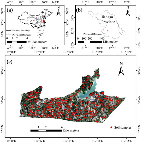
Figure 1.
(a,b) Location of the study area; (c) distribution of sampling points and remote sensing image.
2.2. Soil Data
A total of 223 soil samples (0–20 cm depth) were collected in this study from March 2021 to February 2025. The sampling followed the principles of representativeness and uniformity, ensuring that each sampling point represented a certain area of the soil landscape, including land use, topography, and geomorphology, with similar or consistent characteristics. Additionally, the spatial distribution of all sampling points was relatively uniform across the study area. Based on the USDA soil texture classification standards, the soils were categorized into four types: loam, silty clay, silty clay loam, and silty loam. The spatial distribution of the soil sampling points is shown in Figure 1.
2.3. Environmental Variables Data
According to the theory of soil-forming factors, soil texture is influenced by five major factors: topography, biology, time, soil parent material, and climate [36]. These environmental variables affect or reflect the spatial distribution of soil texture, providing a solid foundation for digital soil mapping.
Typically, climatic factors are suitable for digital soil mapping over large areas. In the study area, which is relatively small, the impact of these variables is limited and they are not readily available. As a result, we excluded them from this study. Field investigations confirmed that the study area contains only a single parent material, which was therefore also excluded.
Considering the characteristics of the study area and the ease of obtaining environmental data, we collected two types of environmental variable data (Figure 2): remote sensing data and topographic data. Additionally, several derivative variables were generated from the remote sensing and topographic data for use in soil texture mapping.
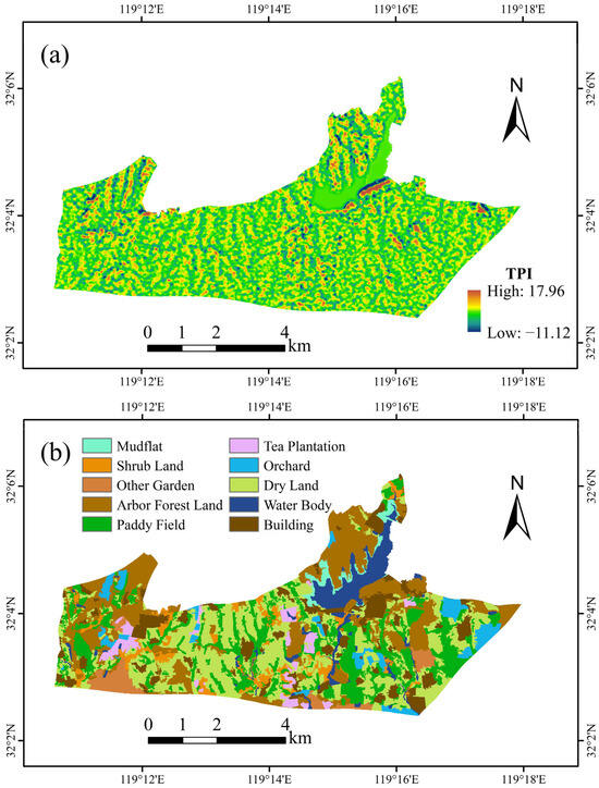
Figure 2.
Main environmental variables maps of the study area: (a) map of terrain position index (TPI); (b) map of land use (LU).
2.3.1. Remote Sensing Data
In the study of soil texture spatial distribution, the application of remote sensing data is of significant importance [37]. The various bands of remote sensing imagery, along with their derived environmental variables, encompass various spectral characteristics that provide rich environmental information for soil texture prediction. These data can reveal subtle surface variations, thereby greatly enhancing the accuracy of soil texture predictions and making the spatial distribution patterns of soil textures clearer and more precise [38]. The remote sensing imagery used in this study was sourced from the GF-2 satellite data provided by the China Centre for Resources Satellite Data and Application (https://data.cresda.cn/#/home, accessed on 10 May 2025), The imagery was captured on 19 September 2019 when there was no cloud cover, ensuring clear and distinguishable surface features. The GF-2 images consist of panchromatic images (0.45–0.90 μm) and multispectral images (near-infrared band: 0.77–0.89 μm; red band: 0.63–0.69 μm; green band: 0.52–0.59 μm; and blue band: 0.45–0.52 μm), The spatial resolution of the multispectral images is 4 m, while the spatial resolution of the panchromatic images is 1 m [39]. The GF-2 images underwent the following preprocessing steps [40]: (1) multispectral images: radiometric calibration, atmospheric correction, orthorectification; (2) panchromatic images: radiometric calibration, orthorectification; and (3) fusion of multispectral and panchromatic images. Based on the fused imagery, several vegetation indices were calculated as environmental variables [41,42], including the Green Leaf Index (GLI), Greenness Ratio Vegetation Index (GRVI), Normalized Difference Vegetation Index (NDVI), Normalized Difference Water Index (NDWI), and Simple Ratio (SR). Additionally, based on GF-2 imagery, we employed a random forest model to generate an initial land use (LU) map. To avoid excessive fragmentation of patches, we merged those smaller than 600 m2 and manually refined the boundaries. The resulting adjusted land use map was then used as an environmental variable. The land use within the study area is classified into 10 categories: cultivated land (paddy field and dry land), forest land (arbor forest land and shrub land), garden (tea plantation, orchard, and other gardens), mudflat, water body, and building. Table 1 presents the environmental variables derived from GF-2 imagery.

Table 1.
Environmental variables derived from GF-2 imagery.
2.3.2. Terrain Data
Topographic features are one of the key factors influencing soil texture variation [49]. The diversity of terrain directly affects the spatial distribution of soil textures. By integrating topographic variables, the accuracy of soil texture spatial distribution maps can be significantly improved [50]. The topographic data used in this study were sourced from the 12.5 m resolution ALOS Digital Elevation Model (DEM) provided by the Alaska Satellite Facility (https://search.asf.alaska.edu/, accessed on 10 May 2025), Based on this data, we calculated eight topographic variables in SAGA-GIS (version 8.4.1), including aspect (Asp), multi-resolution of ridge top flatness index (MRRTF), Multi-Resolution Valley Bottom Flatness Index (MRVBF), plan curvature (PlC), profile curvature (PrC), slope (Slo), terrain position index (TPI), and topographic wetness index (TWI). Additionally, we separately calculated the horizontal distances to the ridge line (HDRL) and to the valley line (HDVL) for further analysis. Table 2 presents the environmental variables derived from ALOS DEM.
Table 2.
Environmental variables derived from ALOS DEM.
2.4. Data Preprocessing
The environmental variables in this study include both factor and numerical types. Among them, LU is a factor environmental variable, which requires one-hot encoding before being used in modeling [55]. The remaining environmental variables are numerical and need to undergo standardization prior to feature selection. The filterVarImp function from the “caret” package in R [56] provides an efficient method for feature selection, especially when selecting variables based on the strength of their relationship with the output. Specifically, a series of cutoff points was applied to the environmental variable data for category prediction. For each cutoff, sensitivity and specificity were computed, which allowed us to construct receiver operating characteristic (ROC) curves and calculate the area under the curve (AUC) for each category using the trapezoidal rule. The maximum AUC was then selected as the importance score for that variable, and the weighted average score was obtained by computing the weighted mean of the importance scores across all categories. In the application of the filterVarImp function, environmental variables with importance scores below 0.6–0.75 [57,58] are generally considered unimportant and may be excluded. In this study, we removed environmental variables with weighted average scores below 0.65, including HDVL, PrC, Asp, and Ele, which are presented in Table 3. The 13 remaining environmental variables selected for analysis are GLI, GRVI, LU, NDVI, NDWI, SR, HDRL, MRRTF, MRVBF, PlC, Slo, TPI, and TWI. All environmental variables in the study area were uniformly resampled to a spatial resolution of 10 m.
Table 3.
Importance scores of the excluded environmental variables calculated using the filterVarImp function.
2.5. Soil Texture Prediction Models
2.5.1. Constrained K-Means Clustering
The Constrained K-Means Clustering is one of the semi-supervised clustering methods [59]. The core idea of semi-supervised clustering is to guide the unsupervised learning process by incorporating a small amount of labeled data [60]. Unlike traditional unsupervised clustering methods, such as K-Means Clustering, which rely solely on the similarity between data points, semi-supervised clustering combines a set of labeled data to enhance the clustering performance.
The Constrained K-Means Clustering [61] generally follows these five steps illustrated in Figure 3:
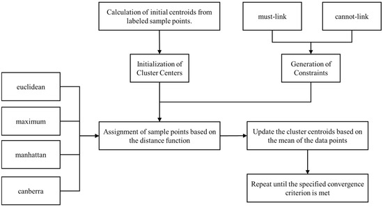
Figure 3.
Flowchart of Constrained K-Means Clustering.
- Initialization of Cluster Centers: For each cluster, the initial center is computed as the mean of the feature vectors of all labeled data points within that category. For instance, when initializing the cluster center for the soil texture type “Loam”, the mean values of the environmental variables for all corresponding labeled samples are calculated to establish the center.
- Generation of Constraints: Constraint information is derived from the labeled data, encompassing both must-link and cannot-link constraints. A must-link constraint indicates that two data points must belong to the same cluster, whereas a cannot-link constraint requires that they belong to different clusters. Specifically, for each soil texture class, a must-link constraint is created between every pair of labeled samples within that class to ensure they are assigned to the same cluster during the clustering process. Conversely, cannot-link constraints are imposed between labeled samples of different classes to guarantee they are assigned to different clusters. For example, if two soil samples are both classified as Loam, they form a must-link pair; conversely, if one sample is classified as Loam and the other as Silty Loam, they form a cannot-link pair. By analogy, must-link constraints and cannot-link constraints were established for all soil sample points.
- Assignment of Data Points: For each unlabeled sample, the distance to every cluster center is calculated, and the sample is assigned to the cluster corresponding to the nearest center. In contrast, the cluster assignments of labeled samples remain unchanged due to the imposed constraints. At this stage, the distance function is a crucial parameter, and its selection can significantly affect the final assignment outcomes. In contrast to conventional supervised classification methods that rely solely on labeled data to build the model, this approach fully exploits a small number of labeled samples in conjunction with a large volume of unlabeled data. In essence, the few labeled samples serve to guide the clustering of the abundant unlabeled samples, ultimately achieving effective classification.
- Updating Cluster Centers: For each cluster, the center is recalculated by computing the mean of all data points within that cluster. The clustering assignments of labeled samples remain fixed due to the constraint information, whereas the assignments for unlabeled samples are continuously updated in subsequent iterations.
- Iterative Optimization: Repeat steps 3 and 4 until the cluster centers no longer change or the maximum number of iterations is reached. In this study, to compare the effect of key parameters (distance method) in Constrained K-Means Clustering, we selected the default number of iterations (i.e., 10 iterations) for each distance method.
K-Means Clustering is sensitive to the initial cluster centers, with different starting points potentially leading to entirely different clustering results [62]. Additionally, K-Means Clustering is highly sensitive to outliers (noise), which can affect the calculation of cluster centers and lead to inaccurate results [63]. Moreover, K-Means Clustering requires the user to predefine the number of clusters.
In Constrained K-Means Clustering, sample points are assigned to the closest cluster based on their distance from the cluster centers, while also considering the imposed constraints [64]. If a must-link constraint exists between two data points, they must be assigned to the same cluster; if a cannot-link constraint exists, they must be assigned to different clusters. The update of cluster centers is also influenced by these constraints. Therefore, unlike K-Means Clustering, Constrained K-Means Clustering can be applied to predict the spatial distribution of soil texture by using must-link and cannot-link constraints. In comparison to conventional machine learning methods, it can effectively utilize and fully leverage large amounts of unlabeled data, enabling predictions even when soil sampling points are sparse.
The advantage of Constrained K-Means Clustering lies in its ability to operate without predefining the number of clusters. By introducing constraint information (such as must-link and cannot-link), it effectively reduces misassignments in clustering, ensuring that the results align more closely with labeled data, especially when labeled data is limited. Furthermore, when dealing with noisy, unlabeled data, the constraints guide the clustering process, preventing the erroneous clustering that can arise with K-Means Clustering and improving the stability of the clustering results [65].
In Constrained K-Means Clustering, the distance method is a key parameter of the model. In this study, we employed four different distance methods [61] to predict the spatial distribution of soil texture and assess the predictive performance of each function. The distance methods used were euclidean, maximum, manhattan, and canberra.
2.5.2. Random Forest (RF)
Random forest (RF) is a classical supervised learning method in machine learning, initially proposed by Breiman [66]. The model utilizes bootstrap sampling to repeatedly select samples for forming prediction sets, and constructs a decision tree for each set, resulting in a total number of trees (ntree). At each node of the decision tree, the number of sample predictors (mtry) is selected as the splitting variable. The input matrix values are processed, and the results from the classification trees are aggregated to form the random forest, which is then used to predict the target variable. In the field of soil mapping, this model has found broad applications, including the prediction of soil types [67], as well as various soil properties, such as soil texture [68,69], soil organic carbon [70], cation exchange capacity [71], and pH [72]. In this study, we performed a 5-fold cross-validation with 10 repetitions to optimize the parameters mtry and ntree, where mtry was set to 4 and ntree to 500.
2.5.3. Multilayer Perceptron (MLP)
The multilayer perceptron (MLP), as a backpropagation-based artificial neural network [73], uses a multi-layered structure for feature extraction and pattern recognition of complex data. The model transforms input data into abstract features through multiple layers of neurons, thereby enabling efficient information processing. At each layer, neurons combine inputs linearly and apply nonlinear activation functions to capture deeper relationships within the data. During MLP model training, the backpropagation algorithm is used to iteratively adjust weights to minimize prediction errors, thereby enhancing predictive accuracy. The MLP model has been widely applied in areas such as image recognition [74] and digital soil mapping [75]. In this study, we optimized the number of hidden layer neurons (size) and the regularization strength parameter (decay) using 10 repetitions of 5-fold cross-validation. The number of hidden neurons was set to 17, and the regularization strength was set to 0.07.
2.6. Assessment of Model Performance
To assess the accuracy and robustness of soil texture predictions, 100 repetitions of cross-validation were performed. A spatial cross-validation scheme was chosen; unlike standard cross-validation, spatial cross-validation addresses spatial autocorrelation. Specifically, a 5-fold spatial blocking strategy was employed, implemented using the R package blockCV [76].
The accuracy of the model is evaluated using three metrics: overall accuracy (), coefficient, and [77,78,79]. The values of , coefficient, and range from 0 to 1, with higher values indicating better predictive performance. The formulas for , coefficient, and are as follows:
where
where , , , and represent true positives, true negatives, false positives, and false negatives, respectively. refers to the probability of agreement when two classes are unconditionally independent. refers to the number of samples correctly predicted as belonging to class by the model. denotes the number of samples from other classes that are incorrectly predicted as belonging to class . refers to the number of samples that truly belong to class but are incorrectly predicted as belonging to other classes by the model. represents the arithmetic mean of the scores across all classes.
2.7. Analysis of Environmental Variable Importance
To evaluate the contribution of environmental variables in the Constrained K-Means Clustering, the silhouette scores [80] were calculated for the spatial distribution of soil textures generated using four different distance methods. Subsequently, each environmental variable was systematically excluded, and the resulting change in the silhouette score was used to assess its importance in the model. A greater change indicates that the variable plays a more significant role in the model.
3. Results
3.1. Descriptive Statistics of Soil Texture Distribution
Table 4 illustrates the distribution pattern of soil textures in the study area. Within the study region, silt is the dominant soil component, exhibiting both high mean and median values; its low coefficient of variation indicates a relatively uniform spatial distribution. Clay content is lower than that of silt, yet it also displays a low coefficient of variation, signifying stable distribution across the region. Sand shows the lowest mean and median values and a comparatively high coefficient of variation, reflecting considerable spatial heterogeneity. Additionally, based on the USDA soil texture classification, the study area consists of four soil texture types: loam, silty clay, silty clay loam, and silty loam. The differences between silty clay, silty clay loam, and silty loam mainly lie in the clay content, while the distinction between loam and the other three soil texture types is primarily based on the silt content. Therefore, the spatial heterogeneity of soil textures in the study area is generally at a low level.
Table 4.
Descriptive statistics for the soil particle fraction.
3.2. Model Predictive Performance
Figure 4 illustrates the prediction performance in soil texture classification using Constrained K-Means Clustering with four different distance methods—euclidean, maximum, manhattan, and canberra—as well as two fully supervised models (RF and MLP). A comparison of the , coefficient, and reveals similar trends across the three methods. In Constrained K-Means Clustering, the euclidean distance method achieved the highest values for , coefficient, and among the four distance methods, with values of 0.77, 0.68, and 0.75, respectively. In contrast, the canberra distance method yielded the lowest , coefficient, and , with values of 0.57, 0.41, and 0.53, respectively. Both the maximum and manhattan distances performed worse than euclidean distance, with , , and values of 0.70, 0.58, and 0.67 and 0.74, 0.64, and 0.72, respectively. The RF and MLP models achieved , , and values of 0.65, 0.50, and 0.63 and 0.59, 0.42, and 0.57, respectively, showing performance that only outperformed the canberra distance and fell short of the other three distance methods. The , , and of the RF and MLP models were 0.12, 0.18, and 0.12 lower, and 0.18, 0.26, and 0.18 lower, respectively, than the euclidean distance method.
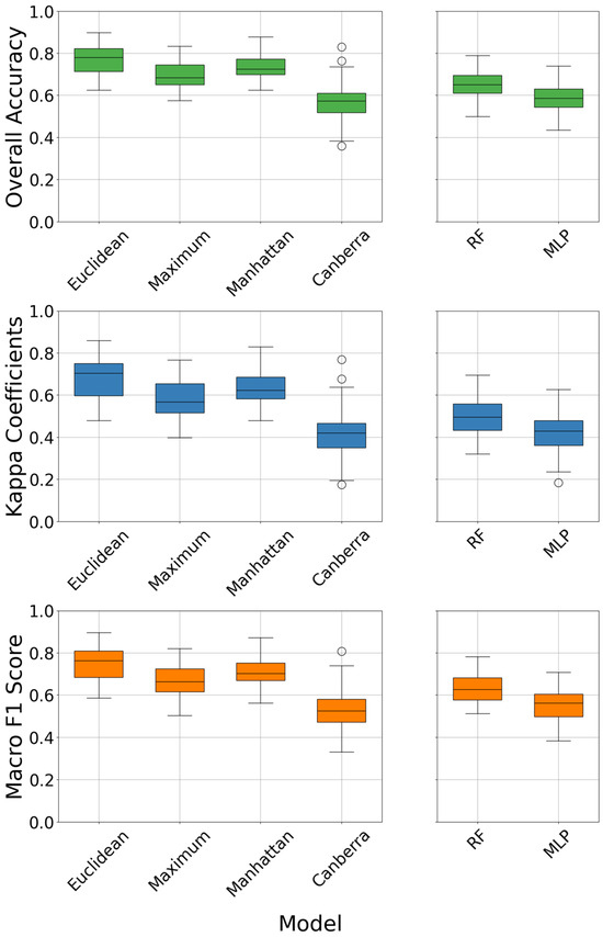
Figure 4.
Overall accuracy (), coefficients, and for several different models.
Overall, among the four distance methods employed in Constrained K-Means Clustering, the euclidean distance method exhibited the most outstanding performance, outperforming both the RF and MLP models and delivering the best prediction accuracy.
3.3. Spatial Distribution of Soil Texture
Figure 5 presents the spatial distribution of soil textures derived from Constrained K-Means Clustering using four different distance methods (euclidean, maximum, manhattan, and canberra) and two fully supervised models (RF and MLP). Overall, the soil texture maps appear largely similar. Notably, loam is predominantly distributed on the upper slopes, where the relative elevation is higher and clay particles have not significantly accumulated. In contrast, the mid-slope areas exhibit the presence of silty clay and silty clay loam; here, silty clay contains a higher clay content than silty clay loam. Compared with the upper slopes, the mid-slope positions are lower, and under the influence of depositional processes, both silt and clay progressively accumulate, leading to the formation of these two soil textures. Among these, silty clay loam is mainly found in dry land, whereas silty clay is largely distributed in areas with denser natural vegetation, such as forest land and garden. This pattern likely results from anthropogenic cultivation or soil amendments in arid regions that slightly reduce clay content, while soils in forest land and garden, being less disturbed, retain their original clay levels. Moreover, silty loam is primarily located in the paddy fields of inter-slope valleys. To ensure proper aeration for rice cultivation, the surface soil in paddy fields typically maintains a relatively low clay content; additionally, due to the combined effects of tillage and persistent waterlogging, clay particles are more prone to being washed away or migrating downward.
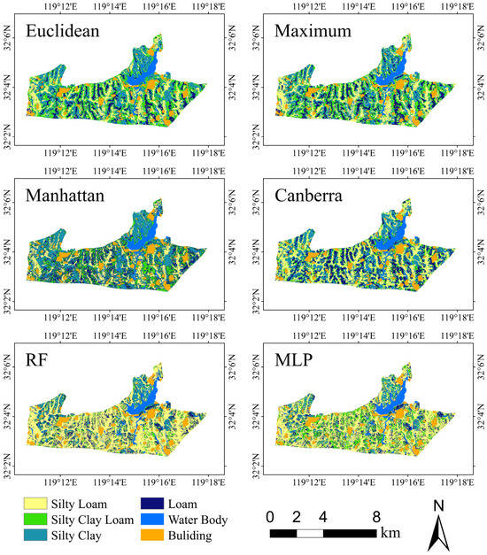
Figure 5.
Spatial distribution maps of soil texture for several different models.
Examining the differences in the resulting spatial distributions reveals that, with the canberra distance, the area classified as loam is noticeably larger than that obtained by the other three distance methods, whereas the distribution of silty clay loam is markedly smaller.
In contrast, the euclidean distance method shows a slightly larger distribution range for silty loam compared to the other three methods. This observation, along with the prediction results for each soil texture category shown in Figure 4, demonstrates that the euclidean distance method exhibits a favorable spatial distribution. Additionally, compared with Constrained K-Means Clustering, the RF and MLP models yield a significantly larger spatial distribution for silty loam and a noticeably smaller distribution for the other soil textures. Furthermore, the spatial distributions of the soil textures produced by the RF and MLP models are considerably more fragmented, underscoring the more coherent and realistic spatial patterns achieved by Constrained K-Means Clustering.
3.4. Importance Analysis of Environmental Variables
Figure 6 illustrates the ranking of environmental variables based on their importance within four clustering methods employed in Constrained K-Means Clustering. The ranking of the importance of each environmental variable across different distance methods is generally consistent. Among the 13 environmental variables examined, LU, MRRTF, TPI, and PlC consistently exhibit high importance in various distance methods. Overall, both remote sensing and topographic variables play crucial roles in the predictive modeling process.
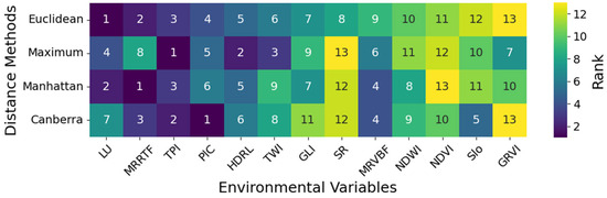
Figure 6.
Ranking of environmental variables based on importance.
Variations in LU lead to changes in soil texture, predominantly due to different vegetation types’ preferences for soil texture, especially in cultivated and other land use types where agricultural practices readily alter soil particle composition, thus accentuating soil texture variability. MRRTF, TPI, and PlC explain soil texture variations from a topographic perspective. Specifically, MRRTF and TPI reflect soil texture changes across different terrain positions, while PlC demonstrates how variations in slope affect the formation of various soil textures.
4. Discussion
Constrained K-Means Clustering, a semi-supervised clustering approach, leverages minimal constraint information such as must-link and cannot-link constraints to guide the clustering process and effectively utilizes a large volume of unlabeled data to predict the spatial distribution of soil texture types. Unlike traditional K-Means Clustering, which merely yields clustering outcomes, Constrained K-Means Clustering utilizes constraint information to correlate labeled soil texture types with cluster categories, enabling pixel-level determination of soil texture types in texture mapping.
This study employs Constrained K-Means Clustering to predict the spatial distribution of soil textures and compares the predictive performance of four distance methods. The choice of distance method significantly impacts performance, underscoring its critical role in the effectiveness of Constrained K-Means Clustering. In addition, we compared the predictive performance of Constrained K-Means Clustering with that of supervised machine learning models—specifically, random forest and multilayer perceptron. The results clearly demonstrate that Constrained K-Means Clustering exhibits a distinct advantage in prediction accuracy. This finding is further supported by other studies. For instance, one study mapping soil texture in central Vietnam using a random forest algorithm on 88 samples reported and coefficients of 0.53 and 0.40, respectively [18]. In another study conducted in northwestern Turkey, decision tree, random forest, and support vector machine models applied to 50 samples yielded and coefficients of 0.57, 0.63, and 0.66, and 0.10, 0.14, and 0.10, respectively [42]. These results further confirm that Constrained K-Means Clustering can achieve superior predictive performance by effectively integrating a small amount of labeled data with a large volume of unlabeled data.
It is important to note that due to its reliance on a distance method, this method has limited capability in handling high-dimensional data and complex nonlinear relationships compared to other machine learning approaches, such as random forest [81,82,83]. However, in typical digital soil mapping applications, where the number of features and sampling points is generally low [84,85], Constrained K-Means Clustering is well-suited and performs robustly. For applications with a large number of soil samples, the abundance of sample data can sufficiently capture the relationship between environmental variables and soil classes. For example, in a study on soil texture classification under vegetative cover [86], a SVM model was employed to predict soil texture classes for 943 samples, achieving an of 0.84 and a coefficient of 0.76, thereby yielding highly accurate results. In such cases, Constrained K-Means Clustering may not demonstrate superior predictive performance, and further research on its potential in this context will be pursued in future studies.
The use of semi-supervised learning methods in digital soil mapping remains uncommon. One notable study in Heshan farm of Nenjiang County in Heilongjiang Province, China, applied a semi-supervised classification approach to limited soil samples [26]. Three base learners—multinomial logistic regression, k-nearest neighbors, and random forest—achieved accuracies of 0.47, 0.50, and 0.55, respectively, while their semi-supervised counterparts reached 0.50, 0.56, and 0.58. Although this represents a measurable improvement, the gains were modest. Moreover, that study randomly selected 10,000 unlabeled samples without accounting for their spatial distribution—for example, by clustering the environmental variables first and then sampling along cluster boundaries or centroids. In contrast, this study uses labeled samples to guide the clustering process and, conceptually, treats the entire set of environmental variable observations as the pool of unlabeled samples.
At present, applications of Constrained K-Means Clustering have been confined to small areas with only a few soil texture classes. Future studies targeting larger regions will encounter a greater diversity of soil texture classes, which may blur distinctions between classes and render conventional distance methods (e.g., euclidean distance) insufficient for discriminating complex patterns. Introducing mahalanobis distance could improve modeling of high-dimensional, nonlinear relationships. Alternatively, transfer learning—such as adapting pre-trained model parameters to new regions—may further enhance scalability.
Overall, it is an effective spatial distribution prediction method that can be applied to predict the spatial distribution of soil texture or other soil properties or types when soil samples are limited.
5. Conclusions
This study employs Constrained K-Means Clustering to integrate remote sensing and topographic environmental variables, using only a limited number of labeled samples alongside abundant unlabeled data to achieve semi-supervised spatial mapping of soil texture under constrained sampling conditions. The predictive performance of the RF and MLP models in soil texture spatial distribution was also compared. The results demonstrate that the Constrained K-Means Clustering effectively combines scarce labeled information with extensive unlabeled data to generate high-accuracy soil texture distribution maps. Within the Constrained K-Means Clustering framework, four distance methods—euclidean, maximum, manhattan, and canberra—were evaluated, with the euclidean distance yielding the best performance and outperforming two fully supervised classification models, RF and MLP. Among the environmental predictors, MRRTF, LU, TPI, and PlC emerged as the most influential variables for soil texture prediction, underscoring their pivotal role in governing the spatial distribution of soil texture types in the study area. Overall, Constrained K-Means Clustering capitalizes on a small set of labeled samples and a large pool of unlabeled samples, demonstrating robust predictive capability and enabling more comprehensive soil texture mapping. This method offers a novel strategy for producing high-precision soil texture maps in cost-sensitive regions without extensive field sampling.
Author Contributions
Conceptualization, F.Z. and J.P.; methodology, F.Z.; software, F.Z.; investigation, F.Z., C.Z., W.L. and Z.F.; data curation, F.Z. and C.Z.; writing—original draft preparation, F.Z. and J.P.; visualization, F.Z., C.Z., Z.F. and W.L. All authors have read and agreed to the published version of the manuscript.
Funding
This research was funded by the National Natural Science Foundation of China, grant number: 41971057.
Data Availability Statement
The original contributions presented in this study are included in the article. Further inquiries can be directed to the corresponding author(s).
Conflicts of Interest
The authors declare no conflicts of interest.
References
- Zheng, M.; Wang, X.; Li, S.; Zhu, B.; Hou, J.; Song, K. Soil Texture Mapping in Songnen Plain of China Using Sentinel-2 Imagery. Remote Sens. 2023, 15, 5351. [Google Scholar] [CrossRef]
- Mallah, S.; Delsouz Khaki, B.; Davatgar, N.; Scholten, T.; Amirian-Chakan, A.; Emadi, M.; Kerry, R.; Mosavi, A.H.; Taghizadeh-Mehrjardi, R. Predicting Soil Textural Classes Using Random Forest Models: Learning from Imbalanced Dataset. Agronomy 2022, 12, 2613. [Google Scholar] [CrossRef]
- Prakash, R.; Singh, D.; Pathak, N.P. Microwave Specular Scattering Response of Soil Texture at X-Band. Adv. Space Res. 2009, 44, 801–814. [Google Scholar] [CrossRef]
- Rajput, U.; Sharma, S.; Swami, D.; Joshi, N. Rapid Assessment of Soil–Water Retention Using Soil Texture-Based Models. Environ. Earth Sci. 2024, 83, 454. [Google Scholar] [CrossRef]
- Silver, W.L.; Neff, J.; McGroddy, M.; Veldkamp, E.; Keller, M.; Cosme, R. Effects of Soil Texture on Belowground Carbon and Nutrient Storage in a Lowland Amazonian Forest Ecosystem. Ecosystems 2000, 3, 193–209. [Google Scholar] [CrossRef]
- Jiang, L.; Liu, H.; Peng, Z.; Dai, J.; Zhao, F.; Chen, Z. Root System Plays an Important Role in Responses of Plant to Drought in the Steppe of China. Land Degrad. Dev. 2021, 32, 3498–3506. [Google Scholar] [CrossRef]
- Zhao, Z.; Feng, W.; Xiao, J.; Liu, X.; Pan, S.; Liang, Z. Rapid and Accurate Prediction of Soil Texture Using an Image-Based Deep Learning Autoencoder Convolutional Neural Network Random Forest (DLAC-CNN-RF) Algorithm. Agronomy 2022, 12, 3063. [Google Scholar] [CrossRef]
- Fan, Y.; Yin, W.; Yang, Z.; Wang, Y.; Ma, L. Moisture Content Distribution Model for the Soil Wetting Body under Moistube Irrigation. Water SA 2023, 49, 73–91. [Google Scholar]
- Ye, C.; Zheng, G.; Tao, Y.; Xu, Y.; Chu, G.; Xu, C.; Chen, S.; Liu, Y.; Zhang, X.; Wang, D. Effect of Soil Texture on Soil Nutrient Status and Rice Nutrient Absorption in Paddy Soils. Agronomy 2024, 14, 1339. [Google Scholar] [CrossRef]
- Fatima, B.; Rachid, H.; Khalil, E.K.; Abdessalam, O.; Abdeldjalil, B.; Mohamed, B.; Tariq, A.; Davis, B.J., Jr.; Soufan, W. Modelling, Quantification and Estimation of the Soil Water Erosion Using the Revised Universal Soil Loss Equation with Sediment Delivery Ratio and the Analytic Hierarchy Process Models. Earth Surf. Process. Landf. 2024, 49, 3158–3176. [Google Scholar] [CrossRef]
- Tolera, A.M.; Haile, M.M.; Merga, T.F.; Feyisa, G.A. Assessment of Land Suitability for Irrigation in West Shewa Zone, Oromia, Ethiopia. Appl. Water Sci. 2023, 13, 112. [Google Scholar] [CrossRef]
- Tosini, L.; Folzer, H.; Heckenroth, A.; Prudent, P.; Santonja, M.; Farnet, A.-M.; Salducci, M.-D.; Vassalo, L.; Labrousse, Y.; Oursel, B.; et al. Gain in Biodiversity but Not in Phytostabilization after 3 Years of Ecological Restoration of Contaminated Mediterranean Soils. Ecol. Eng. 2020, 157, 105998. [Google Scholar] [CrossRef]
- Li, Y.; Wang, L.; Yu, Y.; Zang, D.; Dai, X.; Zheng, S. Cropland Zoning Based on District and County Scales in the Black Soil Region of Northeastern China. Sustainability 2024, 16, 3341. [Google Scholar] [CrossRef]
- Feng, L.; Khalil, U.; Aslam, B.; Ghaffar, B.; Tariq, A.; Jamil, A.; Farhan, M.; Aslam, M.; Soufan, W. Evaluation of Soil Texture Classification from Orthodox Interpolation and Machine Learning Techniques. Environ. Res. 2024, 246, 118075. [Google Scholar] [CrossRef]
- Li, J.; Wan, H.; Shang, S. Comparison of Interpolation Methods for Mapping Layered Soil Particle-Size Fractions and Texture in an Arid Oasis. Catena 2020, 190, 104514. [Google Scholar] [CrossRef]
- Piikki, K.; Söderström, M. Digital Soil Mapping of Arable Land in Sweden—Validation of Performance at Multiple Scales. Geoderma 2019, 352, 342–350. [Google Scholar] [CrossRef]
- Saygın, F.; Aksoy, H.; Alaboz, P.; Dengiz, O. Different Approaches to Estimating Soil Properties for Digital Soil Map Integrated with Machine Learning and Remote Sensing Techniques in a Sub-Humid Ecosystem. Environ. Monit. Assess. 2023, 195, 1061. [Google Scholar] [CrossRef]
- Ngu, N.H.; Thanh, N.N.; Duc, T.T.; Non, D.Q.; Thuy An, N.T.; Chotpantarat, S. Active Learning-Based Random Forest Algorithm Used for Soil Texture Classification Mapping in Central Vietnam. Catena 2024, 234, 107629. [Google Scholar] [CrossRef]
- Silva, S.H.G.; Weindorf, D.C.; Pinto, L.C.; Faria, W.M.; Acerbi, F.W., Jr.; Gomide, L.R.; de Mello, J.M.; de Pádua, A.L., Jr.; Souza, I.A.; Teixeira, A.F.D.S.; et al. Soil Texture Prediction in Tropical Soils: A Portable X-Ray Fluorescence Spectrometry Approach. Geoderma 2020, 362, 114136. [Google Scholar] [CrossRef]
- Yousif, B.S.; Mustafa, Y.T.; Fayyadh, M.A. Digital Mapping of Soil-Texture Classes in Batifa, Kurdistan Region of Iraq, Using Machine-Learning Models. Earth Sci. Inform. 2023, 16, 1687–1700. [Google Scholar] [CrossRef]
- Omondiagbe, O.P.; Lilburne, L.; Licorish, S.A.; MacDonell, S.G. Soil Texture Prediction with Automated Deep Convolutional Neural Networks and Population-Based Learning. Geoderma 2023, 436, 116521. [Google Scholar] [CrossRef]
- Coblinski, J.A.; Giasson, É.; Demattê, J.A.M.; Dotto, A.C.; Costa, J.J.F.; Vašát, R. Prediction of Soil Texture Classes through Different Wavelength Regions of Reflectance Spectroscopy at Various Soil Depths. Catena 2020, 189, 104485. [Google Scholar] [CrossRef]
- Kim, J.; Lee, Y.; Lee, M.-H.; Hong, S.-Y. A Comparative Study of Machine Learning and Spatial Interpolation Methods for Predicting House Prices. Sustainability 2022, 14, 9056. [Google Scholar] [CrossRef]
- Cai, J.; Hao, J.; Yang, H.; Zhao, X.; Yang, Y. A Review on Semi-Supervised Clustering. Inf. Sci. 2023, 632, 164–200. [Google Scholar] [CrossRef]
- Du, F.; Zhu, A.; Liu, J.; Yang, L. Predictive Mapping with Small Field Sample Data Using Semi-supervised Machine Learning. Trans. GIS 2020, 24, 315–331. [Google Scholar] [CrossRef]
- Zhang, L.; Yang, L.; Ma, T.; Shen, F.; Cai, Y.; Zhou, C. A Self-Training Semi-Supervised Machine Learning Method for Predictive Mapping of Soil Classes with Limited Sample Data. Geoderma 2021, 384, 114809. [Google Scholar] [CrossRef]
- Trung, N.T.; Le, X.-H.; Tuan, T.M. Enhancing Contrast of Dark Satellite Images Based on Fuzzy Semi-Supervised Clustering and an Enhancement Operator. Remote Sens. 2023, 15, 1645. [Google Scholar] [CrossRef]
- Roy, P.; Kislay, A.; Plonski, P.A.; Luby, J.; Isler, V. Vision-Based Preharvest Yield Mapping for Apple Orchards. Comput. Electron. Agric. 2019, 164, 104897. [Google Scholar] [CrossRef]
- He, W.; Xiao, Z.; Lu, Q.; Wei, L.; Liu, X. Digital Mapping of Soil Particle Size Fractions in the Loess Plateau, China, Using Environmental Variables and Multivariate Random Forest. Remote Sens. 2024, 16, 785. [Google Scholar] [CrossRef]
- Wang, R.; Chen, W.; Chen, H.; Qin, X. Finer Soil Properties Mapping Framework for Broad-Scale Area: A Case Study of Hubei Province, China. Geoderma 2024, 449, 117023. [Google Scholar] [CrossRef]
- Zhou, Y.; Wu, W.; Liu, H. Exploring the Influencing Factors in Identifying Soil Texture Classes Using Multitemporal Landsat-8 and Sentinel-2 Data. Remote Sens. 2022, 14, 5571. [Google Scholar] [CrossRef]
- Saurette, D.D. Comparing Direct and Indirect Approaches to Predicting Soil Texture Class. Can. J. Soil. Sci. 2022, 102, 835–851. [Google Scholar] [CrossRef]
- Fang, Z.H. Landscape Classification System Based on UAV Images for Soil Survey–A Study Case in Northern of Jurong City. Master’s Thesis, Nanjing Agricultural University, Nanjing, China, 2023. [Google Scholar]
- Zhu, C.; Zhu, F.; Li, C.; Lu, W.; Fang, Z.; Li, Z.; Pan, J. Constructing Soil–Landscape Units Based on Slope Position and Land Use to Improve Soil Prediction Accuracy. Remote Sens. 2024, 16, 4090. [Google Scholar] [CrossRef]
- Zhu, F.; Zhu, C.; Lu, W.; Fang, Z.; Li, Z.; Pan, J. Soil Classification Mapping Using a Combination of Semi-Supervised Classification and Stacking Learning (SSC-SL). Remote Sens. 2024, 16, 405. [Google Scholar] [CrossRef]
- Jenny, H. Factors of Soil Formation: A System of Quantitative Pedology; McGraw-Hill: New York, NY, USA, 1941. [Google Scholar]
- Mirzaeitalarposhti, R.; Shafizadeh-Moghadam, H.; Taghizadeh-Mehrjardi, R.; Demyan, M.S. Digital Soil Texture Mapping and Spatial Transferability of Machine Learning Models Using Sentinel-1, Sentinel-2, and Terrain-Derived Covariates. Remote Sens. 2022, 14, 5909. [Google Scholar] [CrossRef]
- Yüzügüllü, O.; Fajraoui, N.; Liebisch, F. Soil Texture and pH Mapping Using Remote Sensing and Support Sampling. IEEE J. Sel. Top. Appl. Earth Observ. Remote Sens. 2024, 17, 12685–12705. [Google Scholar] [CrossRef]
- Li, Y.; Wang, C.; Wright, A.; Liu, H.; Zhang, H.; Zong, Y. Combination of GF-2 High Spatial Resolution Imagery and Land Surface Factors for Predicting Soil Salinity of Muddy Coasts. Catena 2021, 202, 105304. [Google Scholar] [CrossRef]
- Han, D.; Cao, Y.; Yang, F.; Zhang, X.; Yang, M. Water Quality Estimation Using Gaofen-2 Images Based on UAV Multispectral Data Modeling in Qinba Rugged Terrain Area. Water 2024, 16, 732. [Google Scholar] [CrossRef]
- Tucker, C.J. Red and Photographic Infrared Linear Combinations for Monitoring Vegetation. Remote Sens. Environ. 1979, 8, 127–150. [Google Scholar] [CrossRef]
- Kaya, F.; Başayiğit, L.; Keshavarzi, A.; Francaviglia, R. Digital Mapping for Soil Texture Class Prediction in Northwestern Türkiye by Different Machine Learning Algorithms. Geoderma Reg. 2022, 31, e00584. [Google Scholar] [CrossRef]
- Louhaichi, M.; Borman, M.M.; Johnson, D.E. Spatially Located Platform and Aerial Photography for Documentation of Grazing Impacts on Wheat. Geocarto Int. 2001, 16, 65–70. [Google Scholar] [CrossRef]
- Sripada, R.P.; Heiniger, R.W.; White, J.G.; Meijer, A.D. Aerial Color Infrared Photography for Determining Early In-Season Nitrogen Requirements in Corn. Agron. J. 2006, 98, 968–977. [Google Scholar] [CrossRef]
- Buruso, F.H.; Adimassu, Z.; Sibali, L.L. Effects of Land Use/Land Cover Changes on Soil Properties in Rib Watershed, Ethiopia. Catena 2023, 224, 106977. [Google Scholar] [CrossRef]
- Rouse, J.W.; Haas, R.H.; Schell, J.A.; Deering, D.W. Monitoring Vegetation Systems in the Great Plains with ERTS; Scientific and Technical Information Office, National Aeronautics and Space Administration: Hampton, VA, USA, 1974. [Google Scholar]
- McFeeters, S.K. The use of the Normalized Difference Water Index (NDWI) in the delineation of open water features. Int. J. Remote Sens. 1996, 17, 1425–1432. [Google Scholar] [CrossRef]
- Jordan, C.F. Derivation of Leaf-Area Index from Quality of Light on the Forest Floor. Ecology 1969, 50, 663–666. [Google Scholar] [CrossRef]
- Mirghaed, F.A.; Souri, B. Contribution of Land Use, Soil Properties and Topographic Features for Providing of Ecosystem Services. Ecol. Eng. 2023, 189, 106898. [Google Scholar] [CrossRef]
- Iwashita, F.; Friedel, M.J.; Ribeiro, G.F.; Fraser, S.J. Intelligent Estimation of Spatially Distributed Soil Physical Properties. Geoderma 2012, 170, 1–10. [Google Scholar] [CrossRef]
- Zevenbergen, L.W.; Thorne, C.R. Quantitative analysis of land surface topography. Earth Surf. Process. Landf. 1987, 12, 47–56. [Google Scholar] [CrossRef]
- Gallant, J.C.; Dowling, T.I. A multiresolution index of valley bottom flatness for mapping depositional areas. Water Resour. Res. 2003, 39, 291–297. [Google Scholar] [CrossRef]
- Guisan, A.; Weiss, S.B.; Weiss, A.D. GLM versus CCA spatial modeling of plant species distribution. Plant Ecol. 1999, 143, 107–122. [Google Scholar] [CrossRef]
- Beven, K.J.; Kirkby, M.J. A physically based, variable contributing area model of basin hydrology. Hydrol. Sci. Bull. 1979, 24, 43–69. [Google Scholar] [CrossRef]
- Munaganuri, R.K.; Rao, Y.N. Cap-DiBiL: An Automated Model for Crop Water Requirement Prediction and Suitable Crop Recommendation in Agriculture. Environ. Res. Commun. 2023, 5, 095016. [Google Scholar] [CrossRef]
- Kuhn, M. Caret: Classification and Regression Training. R Package Version 6.0-92. Available online: https://CRAN.R-project.org/package=caret (accessed on 10 May 2025).
- Bonfante, M.C.; Montes, J.C.; Pino, M.; Ruiz, R.; González, G. Machine Learning Applications to Identify Young Offenders Using Data from Cognitive Function Tests. Data 2023, 8, 174. [Google Scholar] [CrossRef]
- Baciu, C.; Ghosh, S.; Naimimohasses, S.; Rahmani, A.; Pasini, E.; Naghibzadeh, M.; Azhie, A.; Bhat, M. Harnessing Metabolites as Serum Biomarkers for Liver Graft Pathology Prediction Using Machine Learning. Metabolites 2024, 14, 254. [Google Scholar] [CrossRef]
- Jia, C.; Guo, L.; Liao, K.; Lu, Z. Efficient Algorithm for the k-Means Problem with Must-Link and Cannot-Link Constraints. Tsinghua Sci. Technol. 2023, 28, 1050–1062. [Google Scholar] [CrossRef]
- Golzari Oskouei, A.; Samadi, N.; Tanha, J. Feature-Weight and Cluster-Weight Learning in Fuzzy c-Means Method for Semi-Supervised Clustering. Appl. Soft Comput. 2024, 161, 111712. [Google Scholar] [CrossRef]
- Basu, S.; Banerjee, A.; Mooney, R.J. Semi-supervised Clustering by Seeding. In Proceedings of the 19th International Conference on Machine Learning (ICML-2002), Sydney, Australia, July 2002. [Google Scholar]
- Yao, G.; Wu, Y.; Huang, X.; Ma, Q.; Du, J. Clustering of Typical Wind Power Scenarios Based on K-Means Clustering Algorithm and Improved Artificial Bee Colony Algorithm. IEEE Access 2022, 10, 98752–98760. [Google Scholar] [CrossRef]
- Zhao, X.; Nie, F.; Wang, R.; Li, X. Improving Projected Fuzzy K-Means Clustering via Robust Learning. Neurocomputing 2022, 491, 34–43. [Google Scholar] [CrossRef]
- Liu, H.; Chen, J.; Dy, J.; Fu, Y. Transforming Complex Problems into K-Means Solutions. IEEE Trans. Pattern Anal. Mach. Intell. 2023, 45, 9149–9168. [Google Scholar] [CrossRef]
- Mei, Y.; Tang, K.; Li, K. Real-Time Identification of Probe Vehicle Trajectories in the Mixed Traffic Corridor. Transp. Res. Part C Emerg. Technol. 2015, 57, 55–67. [Google Scholar] [CrossRef]
- Breiman, L. Random Forests. Mach. Learn. 2001, 45, 5–32. [Google Scholar] [CrossRef]
- Zeraatpisheh, M.; Ayoubi, S.; Jafari, A.; Finke, P. Comparing the Efficiency of Digital and Conventional Soil Mapping to Predict Soil Types in a Semi-Arid Region in Iran. Geomorphology 2017, 285, 186–204. [Google Scholar] [CrossRef]
- Siqueira, R.G.; Moquedace, C.M.; Francelino, M.R.; Schaefer, C.E.G.R.; Fernandes-Filho, E.I. Machine Learning Applied for Antarctic Soil Mapping: Spatial Prediction of Soil Texture for Maritime Antarctica and Northern Antarctic Peninsula. Geoderma 2023, 432, 116405. [Google Scholar] [CrossRef]
- Azizi, K.; Garosi, Y.; Ayoubi, S.; Tajik, S. Integration of Sentinel-1/2 and Topographic Attributes to Predict the Spatial Distribution of Soil Texture Fractions in Some Agricultural Soils of Western Iran. Soil Tillage Res. 2023, 229, 105681. [Google Scholar] [CrossRef]
- Oppong Sarkodie, V.Y.; Vašát, R.; Pouladi, N.; Šrámek, V.; Sáňka, M.; Fadrhonsová, V.; Hellebrandová, K.N.; Borůvka, L. Predicting Soil Organic Carbon Stocks in Different Layers of Forest Soils in the Czech Republic. Geoderma Reg. 2023, 34, e00658. [Google Scholar] [CrossRef]
- Pusch, M.; Samuel-Rosa, A.; Sergio Graziano Magalhães, P.; Rios Do Amaral, L. Covariates in Sample Planning Optimization for Digital Soil Fertility Mapping in Agricultural Areas. Geoderma 2023, 429, 116252. [Google Scholar] [CrossRef]
- Xiao, S.; Ou, M.; Geng, Y.; Zhou, T. Mapping Soil pH Levels across Europe: An Analysis of LUCAS Topsoil Data Using Random Forest Kriging (RFK). Soil Use Manag. 2023, 39, 900–916. [Google Scholar] [CrossRef]
- Rumelhart, D.E.; Hinton, G.E.; Williams, R.J. Learning Internal Representations by Error Propagation. In Parallel Distributed Processing: Explorations in the Microstructure of Cognition, Volume 1: Foundations; Rumelhart, D.E., Mcclelland, J.L., Eds.; MIT Press: Cambridge, MA, USA, 1986; pp. 318–362. [Google Scholar]
- He, X.; Chen, Y. Modifications of the Multi-Layer Perceptron for Hyperspectral Image Classification. Remote Sens. 2021, 13, 3547. [Google Scholar] [CrossRef]
- Chen, S.; Xu, D.; Li, S.; Ji, W.; Yang, M.; Zhou, Y.; Hu, B.; Xu, H.; Shi, Z. Monitoring Soil Organic Carbon in Alpine Soils Using in Situ vis-NIR Spectroscopy and a Multilayer Perceptron. Land Degrad. Dev. 2020, 31, 1026–1038. [Google Scholar] [CrossRef]
- Valavi, R.; Elith, J.; Lahoz-Monfort, J.J.; Flint, I.; Guillera-Arroita, G. blockCV: Spatial and Environmental Blocking for K-Fold and LOO Cross-Validation, R Package Version 2.3.4; CRAN. Available online: https://cran.r-project.org/package=blockCV (accessed on 10 May 2025).
- Wu, W.; Li, A.-D.; He, X.-H.; Ma, R.; Liu, H.-B.; Lv, J.-K. A Comparison of Support Vector Machines, Artificial Neural Network and Classification Tree for Identifying Soil Texture Classes in Southwest China. Computers and Electronics in Agriculture 2018, 144, 86–93. [Google Scholar] [CrossRef]
- Wu, W.; Yang, Q.; Lv, J.; Li, A.; Liu, H. Investigation of Remote Sensing Imageries for Identifying Soil Texture Classes Using Classification Methods. IEEE Trans. Geosci. Remote Sens. 2019, 57, 1653–1663. [Google Scholar] [CrossRef]
- Hong, Y.; Li, D.; Wang, M.; Jiang, H.; Luo, L.; Wu, Y.; Liu, C.; Xie, T.; Zhang, Q.; Jahangir, Z. Cotton Cultivated Area Extraction Based on Multi-Feature Combination and CSSDI under Spatial Constraint. Remote Sens. 2022, 14, 1392. [Google Scholar] [CrossRef]
- Rousseeuw, P.J. Silhouettes: A Graphical Aid to the Interpretation and Validation of Cluster Analysis. J. Comput. Appl. Math. 1987, 20, 53–65. [Google Scholar] [CrossRef]
- Sotomayor, L.N.; Cracknell, M.J.; Musk, R. Supervised Machine Learning for Predicting and Interpreting Dynamic Drivers of Plantation Forest Productivity in Northern Tasmania, Australia. Comput. Electron. Agric. 2023, 209, 107804. [Google Scholar] [CrossRef]
- Ozsagir, M.; Erden, C.; Bol, E.; Sert, S.; Özocak, A. Machine Learning Approaches for Prediction of Fine-Grained Soils Liquefaction. Comput. Geotech. 2022, 152, 105014. [Google Scholar] [CrossRef]
- Sarkar, S.; Ghosh, A.K. On Perfect Clustering of High Dimension, Low Sample Size Data. IEEE Trans. Pattern Anal. Mach. Intell. 2020, 42, 2257–2272. [Google Scholar] [CrossRef]
- Shi, G.; Shangguan, W.; Zhang, Y.; Li, Q.; Wang, C.; Li, L. Reducing Location Error of Legacy Soil Profiles Leads to Improvement in Digital Soil Mapping. Geoderma 2024, 447, 116912. [Google Scholar] [CrossRef]
- Liu, Q.; He, L.; Guo, L.; Wang, M.; Deng, D.; Lv, P.; Wang, R.; Jia, Z.; Hu, Z.; Wu, G.; et al. Digital Mapping of Soil34on Density Using Newly Developed Bare Soil Spectral Indices and Deep Neural Network. Catena 2022, 219, 106603. [Google Scholar] [CrossRef]
- Zhou, Y.; Wu, W.; Wang, H.; Zhang, X.; Yang, C.; Liu, H. Identification of Soil Texture Classes Under Vegetation Cover Based on Sentinel-2 Data with SVM and SHAP Techniques. IEEE J. Sel. Top. Appl. Earth Obs. Remote Sens. 2022, 15, 3758–3770. [Google Scholar] [CrossRef]
Disclaimer/Publisher’s Note: The statements, opinions and data contained in all publications are solely those of the individual author(s) and contributor(s) and not of MDPI and/or the editor(s). MDPI and/or the editor(s) disclaim responsibility for any injury to people or property resulting from any ideas, methods, instructions or products referred to in the content. |
© 2025 by the authors. Licensee MDPI, Basel, Switzerland. This article is an open access article distributed under the terms and conditions of the Creative Commons Attribution (CC BY) license (https://creativecommons.org/licenses/by/4.0/).