
Integration of UAV Remote Sensing and Machine Learning for Taro Blight Monitoring

 , ,
, ,
Abstract
1. Introduction
2. Materials and Methods
2.1. Experimental Design
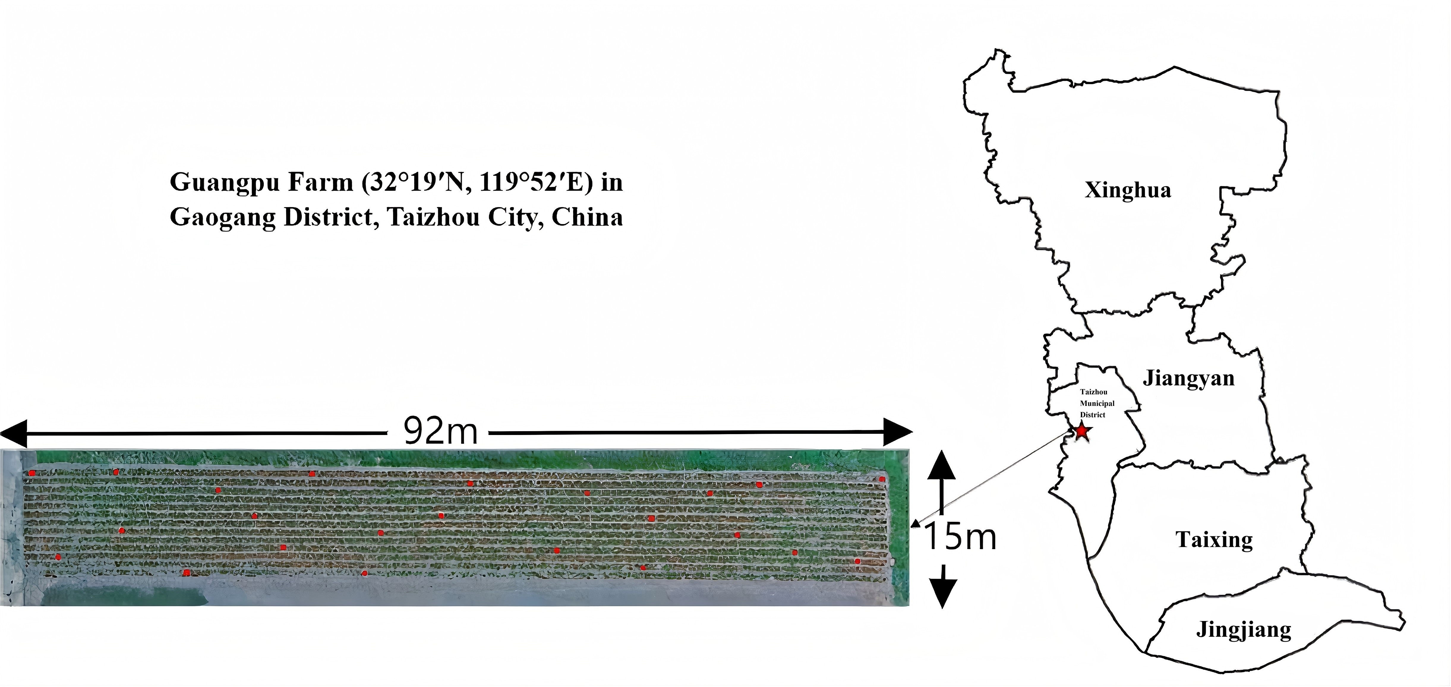
2.1.1. Overview of the Test Area
2.1.2. Field Design
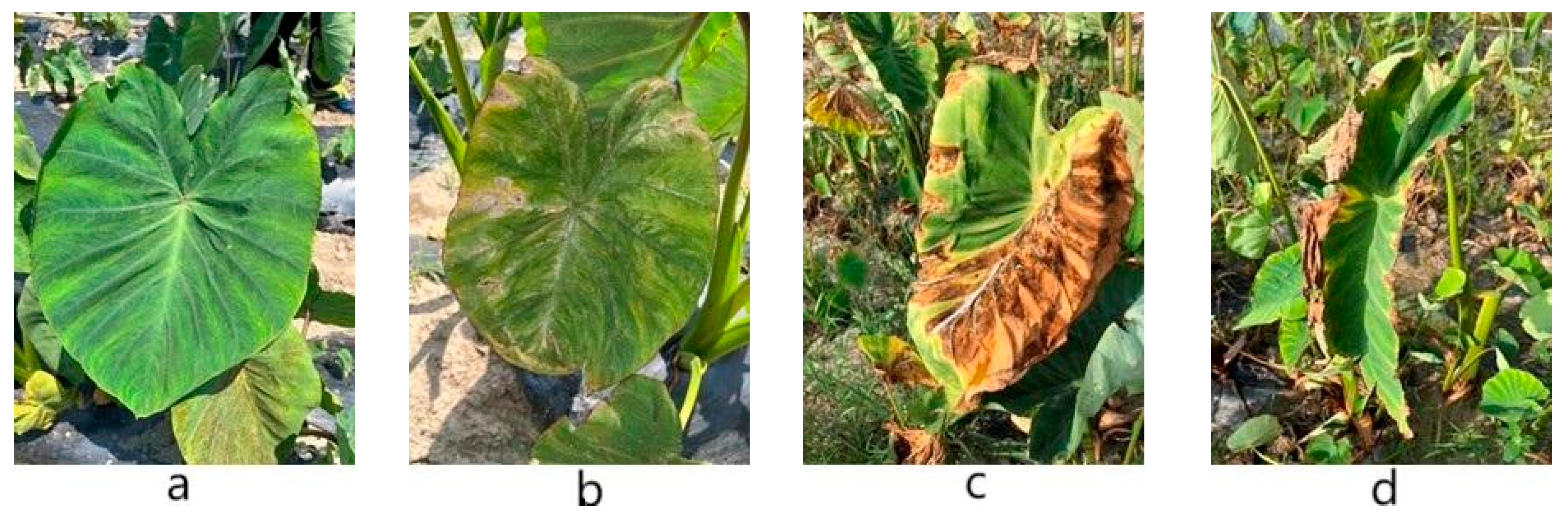
2.2. Field Blight Survey
2.3. Image Data Acquisition
2.3.1. UAV Hyperspectral Image Acquisition Equipment
2.3.2. UAV Multispectral Image Acquisition Equipment
2.3.3. UAV Image Pre-Processing
2.4. Spectral Characteristic Parameters and Vegetation Indices Screening
2.4.1. Hyperspectral Characteristic Parameters Screening
2.4.2. Multispectral Vegetation Indices Screening
2.5. Modeling Methods and Evaluation Indices
2.5.1. Partial Least Squares Regression (PLSR) Algorithm
2.5.2. Random Forest Regression (RFR) Algorithm
2.5.3. Back Propagation Neural Network (BPNN) Algorithm
2.5.4. Model Validation
3. Results
3.1. DI Correlation Analysis of Taro Blight Based on Spectral Information
3.1.1. DI Correlation Analysis of Taro Blight Based on Hyperspectral Characteristic Parameters
3.1.2. Correlation Analysis of Taro Blight DI Based on Multispectral Vegetation Indices
3.2. Taro Blight Estimation Model Based on Hyperspectral Characteristic Parameters
3.2.1. Building and Validation of Taro Blight Estimation Model Based on Partial Least Squares Regression (PLSR)
3.2.2. Building and Validation of Taro Blight Estimation Models Based on Random Forest Regression (RFR)
3.2.3. Building and Validation of Taro Blight Estimation Model Based on Back Propagation Neural Network (BPNN)
3.3. Estimation Model of Taro Blight Based on Multispectral Vegetation Indices
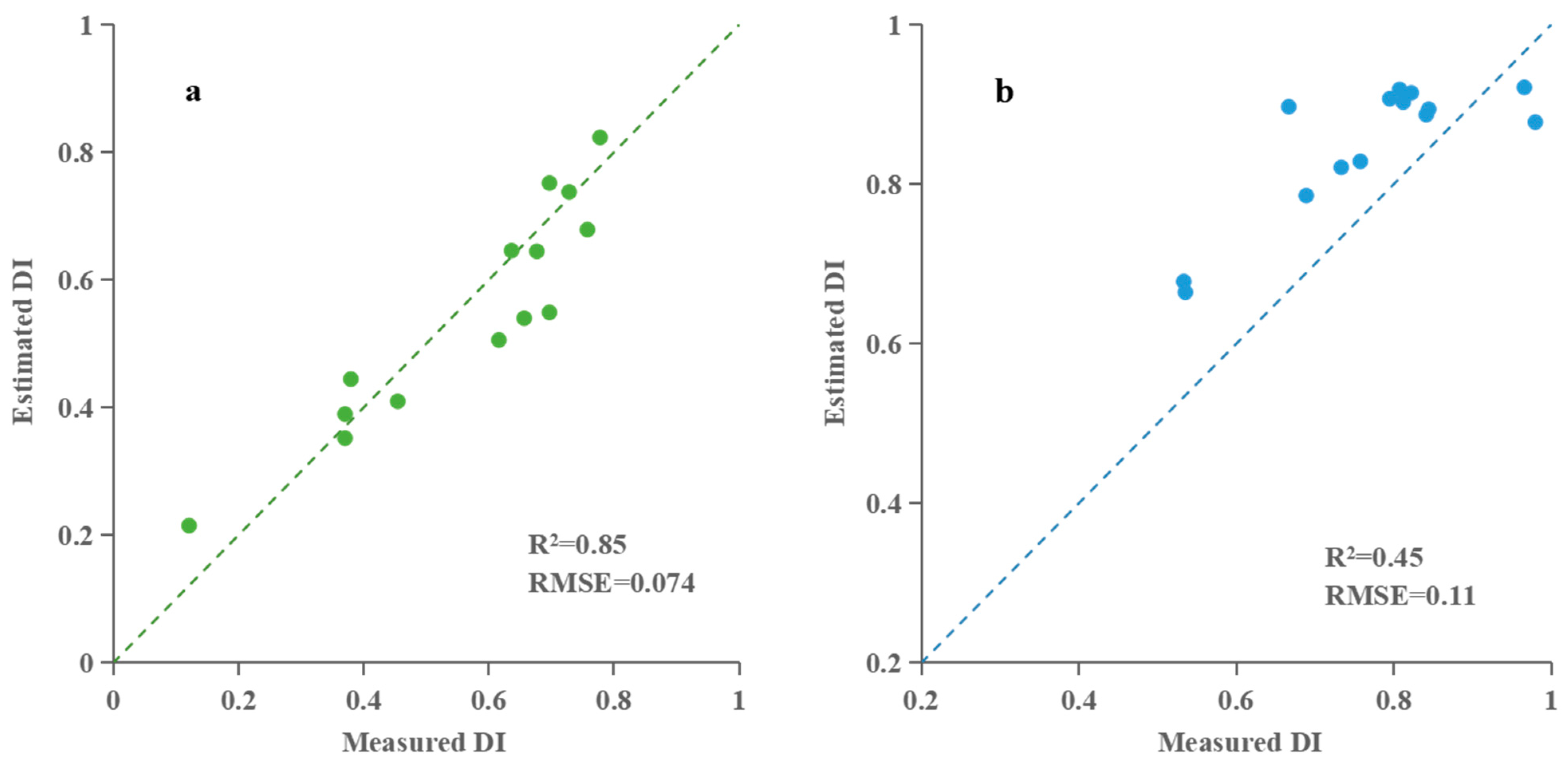
3.3.1. Building and Validation of Taro Blight Estimation Model Based on PLSR
3.3.2. Building and Validation of Taro Blight Estimation Model Based on RFR
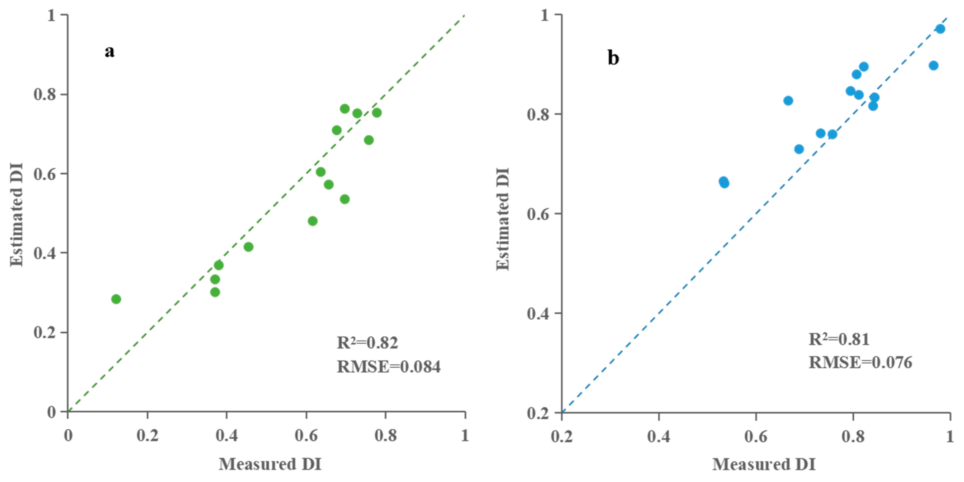
3.3.3. Building and Validation of Taro Blight Estimation Model Based on BPNN
3.4. Comparison of DI Modeling Based on Different Spectral Features
4. Discussion
4.1. Comparison of Taro Canopy Blight Monitoring Based on Spectral Features
4.2. Taro Blight Surveillance Based on UAV Imagery
5. Conclusions
Author Contributions
Funding
Data Availability Statement
Conflicts of Interest
References
- Wang, X.; Chang, L. Development Status of Taro Industry in Taizhou City and Discussion on Its New Business Mode. J. Anhui Agric. Sci. 2018, 46, 196–199. [Google Scholar]
- Sahoo, M.R.; DasGupta, M.; Kole, P.C.; Bhat, J.S.; Mukherjee, A. Antioxidative Enzymes and Isozymes Analysis of Taro Genotypes and Their Implications in Phytophthora Blight Disease Resistance. Mycopathologia 2007, 163, 241–248. [Google Scholar] [CrossRef] [PubMed]
- Brooks, F.E. Detached-Leaf Bioassay for Evaluating Taro Resistance to Phytophthora Colocasiae. Plant Dis. 2008, 92, 126–131. [Google Scholar] [CrossRef]
- Huang, W.; Shi, Y.; Dong, Y.; Ye, H.; Wu, M.; Cui, B.; Liu, L. Progress and Prospects of Crop Diseases and Pests Monitoring by Remote Sensing. Smart Agric. 2019, 1, 1–11. [Google Scholar] [CrossRef]
- Zhu, Y.; Tang, L.; Liu, L.; Liu, B.; Zhang, X.; Qiu, X.; Tian, Y.; Cao, W. Research Progress on the Crop Growth Model CropGrow. Sci. Agric. Sin. 2020, 53, 3235–3256. [Google Scholar] [CrossRef]
- Cheng, T.; Rivard, B.; Sánchez-Azofeifa, G.A.; Feng, J.; Calvo-Polanco, M. Continuous Wavelet Analysis for the Detection of Green Attack Damage due to Mountain Pine Beetle Infestation. Remote Sens. Environ. 2010, 114, 899–910. [Google Scholar] [CrossRef]
- Zhang, J.; Luo, J.; Huang, W.; Wang, J. Continuous Wavelet Analysis Based Spectral Features Selection for Winter Wheat Yellow Rust Detection. Intell. Autom. Soft Comput. 2011, 17, 531–540. [Google Scholar] [CrossRef]
- Zhang, J.; Pu, R.; Huang, W.; Yuan, L.; Luo, J.; Wang, J. Using In-Situ Hyperspectral Data for Detecting and Discriminating Yellow Rust Disease from Nutrient Stresses. Field Crops Res. 2012, 134, 165–174. [Google Scholar] [CrossRef]
- Zhang, J.; Pu, R.; Wang, J.; Huang, W.; Yuan, L.; Luo, J. Detecting Powdery Mildew of Winter Wheat Using Leaf Level Hyperspectral Measurements. Comput. Electron. Agric. 2012, 85, 13–23. [Google Scholar] [CrossRef]
- Zhang, J.; Yuan, L.; Wang, J.; Luo, J.; Du, S.; Huang, W. Research Progress of Crop Diseases and Pests Monitoring Based on Remote Sensing. Trans. Chin. Soc. Agric. Eng. 2012, 28, 1–11. [Google Scholar]
- Liu, H.; Kang, R.; Ustin, S.; Zhang, X.; Fu, Q.; Sheng, L.; Sun, T. Study on the Prediction of Cotton Yield within Field Scale with Time Series Hyperspectral Imagery. Spectrosc. Spectral Anal. 2016, 36, 2585–2589. [Google Scholar]
- Qiao, H.; Zhou, Y.; Bai, Y.; Cheng, D.; Duan, X. The Primary Research of Detecting Wheat Powdery Mildew Using In-Field and Low Altitude Remote Sensing. Acta Phytophylacica Sin. 2006, 33, 341–344. [Google Scholar]
- Backoulou, G.F.; Elliott, N.C.; Giles, K.; Phoofolo, M.; Catana, V.; Mirik, M.; Michels, J. Spatially Discriminating Russian Wheat Aphid Induced Plant Stress from Other Wheat Stressing Factors. Comput. Electron. Agric. 2011, 78, 123–129. [Google Scholar] [CrossRef]
- Liu, W.; Yang, G.; Xu, F.; Qiao, H.; Fan, J.; Song, Y.; Zhou, Y. Comparisons of Detection of Wheat Stripe Rust Using Hyper-Spectrometer and UAV Aerial Photography. Acta Phytopathol. Sin. 2018, 48, 223–227. [Google Scholar] [CrossRef]
- Wang, Z.; Chu, G.; Zhang, H.; Liu, S.; Huang, X.; Gao, F.; Zhang, C.; Wang, J. Identification of Diseased Empty Rice Panicles Based on Haar-like Feature of UAV Optical Image. Trans. Chin. Soc. Agric. Eng. 2018, 34, 73–82. [Google Scholar] [CrossRef]
- Xavier, T.W.F.; Souto, R.N.V.; Statella, T.; Galbieri, R.; Santos, E.S.; Suli, G.S.; Zeilhofer, P. Identification of Ramularia Leaf Blight Cotton Disease Infection Levels by Multispectral, Multiscale UAV Imagery. Drones 2019, 3, 33. [Google Scholar] [CrossRef]
- Portela, F.; Sousa, J.J.; Araújo-Paredes, C.; Peres, E.; Morais, R.; Pádua, L. Monitoring the Progression of Downy Mildew on Vineyards Using Multi-Temporal Unmanned Aerial Vehicle Multispectral Data. Agronomy 2025, 15, 934. [Google Scholar] [CrossRef]
- Li, W.; Guo, Y.; Yang, W.; Huang, L.; Zhang, J.; Peng, J.; Lan, Y. Severity Assessment of Cotton Canopy Verticillium Wilt by Machine Learning Based on Feature Selection and Optimization Algorithm Using UAV Hyperspectral Data. Remote Sens. 2024, 16, 4637. [Google Scholar] [CrossRef]
- Liu, L.; Huang, M.; Huang, W.; Wang, J.; Zhao, C.; Zheng, L.; Tong, Q. Monitoring Stripe Rust Disease of Winter Wheat Using Multi-Temporal Hyperspectral Airborne Data. J. Remote Sens. 2004, 8, 275–281. [Google Scholar] [CrossRef]
- Li, X.; Lee, W.S.; Li, M.; Ehsani, R.; Mishra, A.K.; Yang, C.; Mangan, R.L. Spectral Difference Analysis and Airborne Imaging Classification for Citrus Greening Infected Trees. Comput. Electron. Agric. 2012, 83, 32–46. [Google Scholar] [CrossRef]
- Severtson, D.; Callow, N.; Flower, K.; Neuhaus, A.; Olejnik, M.; Nansen, C. Unmanned Aerial Vehicle Canopy Reflectance Data Detects Potassium Deficiency and Green Peach Aphid Susceptibility in Canola. Precis. Agric. 2016, 17, 659–677. [Google Scholar] [CrossRef]
- Sugiura, R.; Tsuda, S.; Tamiya, S.; Itoh, A.; Nishiwaki, K.; Murakami, N.; Shibuya, Y.; Hirafuji, M.; Nuske, S. Field Phenotyping System for the Assessment of Potato Late Blight Resistance Using RGB Imagery from an Unmanned Aerial Vehicle. Biosyst. Eng. 2016, 148, 1–10. [Google Scholar] [CrossRef]
- Su, J.; Liu, C.; Coombes, M.; Hu, X.; Wang, C.; Xu, X.; Li, Q.; Guo, L.; Chen, W.-H. Wheat Yellow Rust Monitoring by Learning from Multispectral UAV Aerial Imagery. Comput. Electron. Agric. 2018, 155, 157–166. [Google Scholar] [CrossRef]
- Edna Chebet, T.; Li, Y.; Sam, N.; Liu, Y. A Comparative Study of Fine-Tuning Deep Learning Models for Plant Disease Identification. Comput. Electron. Agric. 2019, 161, 272–279. [Google Scholar] [CrossRef]
- Li, Y.; Chang, Q.; Liu, X.; Yan, L.; Luo, D.; Wang, S. Estimation of Maize Leaf SPAD Value Based on Hyperspectrum and BP Neural Network. Trans. Chin. Soc. Agric. Eng. 2016, 32, 135–142. [Google Scholar] [CrossRef]
- Han, Y.; Liu, H.; Zhang, X.; Yu, Z.; Meng, X.; Kong, F.; Song, S.; Han, J. Prediction Model of Rice Panicles Blast Disease Degree Based on Canopy Hyperspectral Reflectance. Spectrosc. Spectral Anal. 2021, 41, 1220–1226. [Google Scholar]
- Gitelson, A.A.; Merzlyak, M.N.; Chivkunova, O.B. Optical Properties and Nondestructive Estimation of Anthocyanin Content in Plant Leaves. Photochem. Photobiol. 2001, 74, 38–45. [Google Scholar] [CrossRef]
- Zhou, J.; Yungbluth, D.; Vong, C.N.; Scaboo, A.; Zhou, J. Estimation of the Maturity Date of Soybean Breeding Lines Using UAV-Based Multispectral Imagery. Remote Sens. 2019, 11, 2075. [Google Scholar] [CrossRef]
- Liu, D.; Wen, D.; Zhu, J. Object-Oriented Land Use Information Extraction Based on UAV Images. Geospatial Inf. 2020, 18, 75–80. [Google Scholar] [CrossRef]
- Zhang, L.; Chen, Y.; Li, Y.; Ma, J.; Du, K.; Zheng, F.; Sun, Z. Estimating above Ground Biomass of Winter Wheat at Early Growth Stages Based on Visual Spectral. Spectrosc. Spectral Anal. 2019, 39, 2501–2506. [Google Scholar]
- Steele, M.R.; Gitelson, A.A.; Rundquist, D.C.; Merzlyak, M.N. Nondestructive Estimation of Anthocyanin Content in Grapevine Leaves. Am. J. Enol. Vitic. 2009, 60, 87–92. [Google Scholar] [CrossRef]
- Haboudane, D.; Miller, J.R.; Tremblay, N.; Zarco-Tejada, P.J.; Dextraze, L. Integrated Narrow-Band Vegetation Indices for Prediction of Crop Chlorophyll Content for Application to Precision Agriculture. Remote Sens. Environ. 2002, 81, 416–426. [Google Scholar] [CrossRef]
- Zarco-Tejada, P.J.; Berjón, A.; López-Lozano, R.; Miller, J.R.; Martín, P.; Cachorro, V.; González, M.R.; de Frutos, A. Assessing Vineyard Condition with Hyperspectral Indices: Leaf and Canopy Reflectance Simulation in a Row-Structured Discontinuous Canopy. Remote Sens. Environ. 2005, 99, 271–287. [Google Scholar] [CrossRef]
- Lv, Y.; Lv, W.; Han, K.; Tao, W.; Zheng, L.; Weng, S.; Huang, L. Determination of Wheat Kernels Damaged by Fusarium Head Blight Using Monochromatic Images of Effective Wavelengths from Hyperspectral Imaging Coupled with an Architecture Self-Search Deep Network. Food Control 2022, 135, 108819. [Google Scholar] [CrossRef]
- Maimouni, S.; Bannari, A.; El-Harti, A.; El-Ghmari, A. Potentiels et Limites Des Indices Spectraux Pour Caractériser La Dégradation Des Sols En Milieu Semi-Aride. Can. J. Remote Sens. 2011, 37, 285–301. [Google Scholar] [CrossRef]
- Juliane, B.; Kang, Y.; Helge, A.; Andreas, B.; Simon, B.; Janis, B.; Martin, L.G.; Georg, B. Combining UAV-Based Plant Height from Crop Surface Models, Visible, and near Infrared Vegetation Indices for Biomass Monitoring in Barley. Int. J. Appl. Earth Obs. Geoinf. 2015, 39, 79–87. [Google Scholar] [CrossRef]
- Zhang, J.; Qiu, X.; Wu, Y.; Zhu, Y.; Cao, Q.; Liu, X.; Cao, W. Combining Texture, Color, and Vegetation Indices from Fixed-Wing UAS Imagery to Estimate Wheat Growth Parameters Using Multivariate Regression Methods. Comput. Electron. Agric. 2021, 185, 106138. [Google Scholar] [CrossRef]
- Haralick, R.M.; Shanmugam, K.; Dinstein, I. Textural Features for Image Classification. IEEE Trans. Syst. Man Cybern. 1973, 3, 610–621. [Google Scholar] [CrossRef]
- Sims, D.A.; Gamon, J.A. Relationships between Leaf Pigment Content and Spectral Reflectance across a Wide Range of Species, Leaf Structures and Developmental Stages. Remote Sens. Environ. 2002, 81, 337–354. [Google Scholar] [CrossRef]
- Gitelson, A.A.; Dall’Olmo, G.; Moses, W.; Rundquist, D.C.; Barrow, T.; Fisher, T.R.; Gurlin, D.; Holz, J. A Simple Semi-Analytical Model for Remote Estimation of Chlorophyll-a in Turbid Waters: Validation. Remote Sens. Environ. 2008, 112, 3582–3593. [Google Scholar] [CrossRef]
- Naidu, R.A.; Perry, E.M.; Pierce, F.J.; Mekuria, T. The Potential of Spectral Reflectance Technique for the Detection of Grapevine Leafroll-Associated Virus-3 in Two Red-Berried Wine Grape Cultivars. Comput. Electron. Agric. 2009, 66, 38–45. [Google Scholar] [CrossRef]
- Mahlein, A.-K.; Rumpf, T.; Welke, P.; Dehne, H.-W.; Plümer, L.; Steiner, U.; Oerke, E.-C. Development of Spectral Indices for Detecting and Identifying Plant Diseases. Remote Sens. Environ. 2013, 128, 21–30. [Google Scholar] [CrossRef]
- Huang, L.; Zhang, H.; Ruan, C.; Huang, W.; Zhao, J. Detection of Scab in Wheat Ears Using in Situ Hyperspectral Data and Support Vector Machine Optimized by Genetic Algorithm. Int. J. Agric. Biol. Eng. 2020, 13, 182–188. [Google Scholar] [CrossRef]
- Wessman, C.A.; Aber, J.D.; Peterson, D.L. An Evaluation of Imaging Spectrometry for Estimating Forest Canopy Chemistry. Int. J. Remote Sens. 1989, 10, 1293–1316. [Google Scholar] [CrossRef]
- Gitelson, A.A.; Kaufman, Y.J.; Merzlyak, M.N. Use of a Green Channel in Remote Sensing of Global Vegetation from EOS-MODIS. Remote Sens. Environ. 1996, 58, 289–298. [Google Scholar] [CrossRef]
- Merzlyak, M.N.; Gitelson, A.A.; Chivkunova, O.B.; Rakitin, V.Y. Non-Destructive Optical Detection of Pigment Changes during Leaf Senescence and Fruit Ripening. Physiol. Plant. 1999, 106, 135–141. [Google Scholar] [CrossRef]
- Imhoff, M.L.; Bounoua, L.; DeFries, R.; Lawrence, W.T.; Stutzer, D.; Tucker, C.J.; Ricketts, T. The Consequences of Urban Land Transformation on Net Primary Productivity in the United States. Remote Sens. Environ. 2004, 89, 434–443. [Google Scholar] [CrossRef]
- Patrick, A.; Pelham, S.; Culbreath, A.; Holbrook, C.C.; De Godoy, I.J.; Li, C. High Throughput Phenotyping of Tomato Spot Wilt Disease in Peanuts Using Unmanned Aerial Systems and Multispectral Imaging. IEEE Instrum. Meas. Mag. 2017, 20, 4–12. [Google Scholar] [CrossRef]
- Guo, A.; Huang, W.; Dong, Y.; Ye, H.; Ma, H.; Liu, B.; Wu, W.; Ren, Y.; Ruan, C.; Geng, Y. Wheat Yellow Rust Detection Using UAV-Based Hyperspectral Technology. Remote Sens. 2021, 13, 123. [Google Scholar] [CrossRef]
- Cui, Y. The Progress of Leaf Blight Research in Taro. China Plant Prot. 2020, 40, 22–26+38. [Google Scholar]
- Yuan, H.; Zhang, F.; Wang, X.; Wu, X.; Yang, Y. Influencing Factors and Control Measures of Rugao Xiangtang Taro Blight. China Plant Prot. 2018, 38, 52–56. [Google Scholar]
- Feng, H.; Hong, Q.; Hu, C.; Huang, W.; Hu, X.; Liu, J.; Zhang, Y.; Zhang, Z.; Qiao, H.; Liu, W. Recent Advances in Intelligent Techniques for Monitoring and Prediction of Crop Diseases and Insect Pests in China. Plant Prot. 2023, 49, 229–242. [Google Scholar] [CrossRef]
- Guo, W.; Zhu, Y.; Wang, H.; Zhang, J.; Dong, P.; Qiao, H. Monitoring Model of Winter Wheat Take-All Based on UAV Hyperspectral Imaging. Trans. Chin. Soc. Agric. Mach. 2019, 50, 162–169. [Google Scholar] [CrossRef]
- Su, B.; Liu, Y.; Huang, Y.; Wei, R.; Cao, X.; Han, D. Analysis for Stripe Rust Dynamics in Wheat Population Using UAV Remote Sensing. Trans. Chin. Soc. Agric. Eng. 2021, 37, 127–135. [Google Scholar] [CrossRef]
- Feng, Z.; Song, L.; Zhang, S.; Jing, Y.; Duan, J.; He, L.; Yin, F.; Feng, W. Wheat Powdery Mildew Monitoring Based on Information Fusion of Multi-Spectral and Thermal Infrared Images Acquired with an Unmanned Aerial Vehicle. Sci. Agric. Sin. 2022, 55, 890–906. [Google Scholar] [CrossRef]
- Shen, W.; Li, Y.; Feng, W.; Zhang, H.; Zhang, Y.; Xie, Y.; Guo, T. Inversion Model for Severity of Powdery Mildew in Wheat Leaves Based on Factor Analysis-BP Neural Network. Trans. Chin. Soc. Agric. Eng. 2015, 31, 183–190. [Google Scholar] [CrossRef]
- Liu, L.; Dong, Y.; Huang, W.; Du, X.; Ma, H. Monitoring Wheat Fusarium Head Blight Using Unmanned Aerial Vehicle Hyperspectral Imagery. Remote Sens. 2020, 12, 3811. [Google Scholar] [CrossRef]
- Wang, H.; Yu, S.; Zhang, H.; Zhao, Y. Taro Blight: Spatial Distribution Pattern and Sampling Technique. Chin. Agric. Sci. Bull. 2020, 36, 118–122. [Google Scholar] [CrossRef]
- Nie, J.; Jiang, J.; Li, Y.; Li, J.; Chao, X.; Ercisli, S. Efficient Detection of Cotton Verticillium Wilt by Combining Satellite Time-Series Data and Multiview UAV Images. IEEE J. Sel. Top. Appl. Earth Observ. Remote Sens. 2024, 17, 13547–13557. [Google Scholar] [CrossRef]


| Disease Level | Grading Standard (In Plants) |
|---|---|
| 0 | Disease-free |
| 1 | Sporadic necrotic spots |
| 2 | Necrotic area not exceeding 1/4 of leaf area |
| 3 | Necrotic area covering 1/4 to 1/3 of leaf area |
| 4 | Necrotic area covering 1/3 to 2/3 of leaf area |
| 5 | Necrotic area covering more than 2/3 of leaf area |
| Technology Name | Specific Parameters |
|---|---|
| Take-Off Weight | 9.5 kg |
| Diagonal Wheelbase | 1133 mm |
| Max Pitch Angle | 25° |
| Operating Temperature | −10 °C to 40 °C |
| Hover Time | 32 min (no load) 16 min (6 kg load) |
| Hover Accuracy | Vertical: ±0.5 m Horizontal: ±1.5 m |
| Technology Name | Specific Parameter | Technology Name | Specific Parameter |
|---|---|---|---|
| Spectral Range | 400~1000 (1 nm) | Field of View (FOV) | 31.34°@16 mm |
| Spectral Resolution | 3.5 nm@30 µm slit | Horizontal Field of View (flight altitude 300 m) | 168 m@16 mm |
| Numerical Aperture | F/2.8 | Lens | 16 mm/23 mm/25 mm |
| Spectral Sampling Rate | 0.7 nm | Number of Spectral Channels | 1040 (1X)/520(2X) 256 (4X)/128 (8X) |
| Full-Width Pixel | 1392 × 1040 | Spatial Resolution | 0.12 |
| Pixel Pitch | 6.45 (µm) | Camera Out | 14 (bit) |
| Technology Name | Specific Parameter |
|---|---|
| Take-Off Weight | 1487 g |
| Diagonal Size (Propellers Excluded) | 350 mm |
| Flight Time | 27 min |
| Operating Frequency | 5.725 GHz to 5.850 GHz |
| Hover Accuracy | Vertical: ±0.1 m Horizontal: ±0.1 m |
| Technology Name | Specific Parameter | Technology Name | Specific Parameter |
|---|---|---|---|
| Max Photo Resolution | 1600 × 1300 (4:3.25) | ISO Range | 200~800 |
| Lens | FOV: 62.7° Focal Length: 5.74 mm Aperture: f/2.2 | Electronic Global Shutter | 1/100~1/20,000 s (visible light) 1/100~1/10,000 s(multispectral) |
| Photo Format | JPEG + TIFF | Monochromatic Sensor Gain | 1 to 8 times |
| Type | Parameter Name | Abridge | Expression and Extraction Method | References |
|---|---|---|---|---|
| Three-Edge Parameter | Blue edge amplitude | Db | The maximum value of the first derivative spectrum at wavelengths 490~530 nm | [24] |
| Yellow edge amplitude | Dy | The maximum value of the first derivative spectrum at wavelengths 560~640 nm | [24] | |
| Red edge amplitude | Dr | The maximum value of the first derivative spectrum at wavelengths 680~760 nm | [24] | |
| Blue edge area | SDb | Integration of first derivative spectra at wavelengths 490~530 nm | [24] | |
| Yellow edge area | SDy | Integration of first derivative spectra at wavelengths 560~640 nm | [24] | |
| Red edge area | SDr | Integration of first derivative spectra at wavelengths 680~760 nm | [24] | |
| Red valley value | Ρr | The minimum value of the original spectrum at wavelength 640~680 nm | [24] | |
| Green peak value | Ρg | The maximum value of the original spectrum at wavelength 510~560 nm | [24] | |
| Green peak area | SDg | Integration of original spectra at wavelengths 510~560 nm | [24] | |
| - | ρg/ρr | The ratio of the green peak value to the red valley value | [25] | |
| - | (ρg − ρr)/ (ρg + ρr) | The normalized value for the green peak value and red valley value | [25] | |
| Three-Edge Parameter | - | SDr/SDb | The ratio of the red edge area to the blue edge area | [25] |
| - | SDr/Sdy | The ratio of the red edge area to the yellow edge area | [25] | |
| - | (SDr − SDb)/ (SDr + SDb) | Normalized ratio of red edge area to blue edge area | [25] | |
| - | (SDr − SDy)/ (SDr + SDy) | Normalized ratio of red edge area to yellow edge area | [25] | |
| Absorption Valley Parameters | Absorption valley area | A | Integration of absorption valleys in continuum removal spectra | [26] |
| Absorption valley width | W | Distance on either side of absorption valley at half-depth | [26] | |
| Absorption valley depth | DP | Distance from the lowest point of absorption valley to the baseline | [26] | |
| Absorption valley left slope | SL | The slope of the connecting line between the left starting point of the absorption valley and the bottom point of the absorption valley | [26] | |
| Absorption valley right slope | SR | The slope of the connecting line between the right starting point of the absorption valley and the bottom point of the absorption valley | [26] |
| Parameter Name | Abridge | Expression and Extraction Method | References |
|---|---|---|---|
| Anthocyanin Reflectance Index | ARI | 1/g − 1/r | [27] |
| Coloration Index | CI | (r − b)/r | [28] |
| Combination Indices | COM | 0.25EXG + 0.3EXGR + 0.33CIVE + 0.12VEG | [29] |
| Extra Green–Red Difference Index | EXGR | EXG − EXR | [30] |
| Extra Red Vegetation Index | EXR | 1.4r − g | [30] |
| Greenness Index | GI | g/r | [31,32,33] |
| Green Leaf Index | GLI | (2g − b − r)/(2g + b+r) | [34] |
| Hue | H | Arctan((2r − g − b)/3.5*(g − b)) | [27] |
| Indice de Forme | IF | (2r − g − b)/(g − b) | [35] |
| Red Green Ratio Index | IGR | r − b | [27] |
| Modified Green–Red Vegetation Index | MGRVI | (g2 − r2)/(g2 + r2) | [36] |
| Normalized Green–Red Difference Index | NGRDI | (g − r)/(g + r) | [37] |
| Red, Green, and Blue Vegetation Index | RGBVI | (g2 − br)/(g2 + br) | [38] |
| Red–Green Ratio | RGR | r/g | [39] |
| Visible Atmospherically Resistant Index in Green Band | VARIgreen | (g − r)/(g + r − b) | [40,41] |
| Chlorotic Leaf Spot Index | CLSI | (re − g)/(tr − g) − re | [42] |
| Modified Simple Ratio | MSR | r/(nir/r + 1)^0.5 | [43] |
| Normalized Difference Vegetation Index | NDVI | (nir − r)/(nir + r) | [44] |
| Normalized Difference Vegetation Index of Red Edge | NDVIrededge | (re − r)/(re + r) | [45] |
| Plant Senescence Reflectance Index | PSRI | (re − g)/nir | [46] |
| Red and Blue Normalized Difference Vegetation Index | RBNDVI | (nir − (r + b))/(nir + (r + b)) | [27] |
| Red Red Edge Ratio Index 2 | RRI2 | re/r | [27] |
| Ratio Vegetation Index | RVI | nir/r | [47] |
| Woebbecke Index | WI | (g − b)/(re − b) | [48] |
| Characteristic Parameter | Correlation Coefficient | Ranking | Characteristic Parameter | Correlation Coefficient | Ranking |
|---|---|---|---|---|---|
| Db | −0.318 * | 26 | A1 | 0.621 ** | 18 |
| Dy | −0.441 ** | 23 | A2 | 0.81 ** | 9 |
| Dr | 0.627 ** | 17 | A3 | 0.856 ** | 1 |
| SDb | 0.021 | 30 | W1 | −0.384 * | 25 |
| SDy | 0.819 ** | 6 | W2 | −0.855 ** | 2 |
| SDr | −0.814 ** | 7 | W3 | −0.224 | 27 |
| Ρr | 0.603 ** | 19 | DP1 | 0.683 ** | 14 |
| Ρg | 0.434 ** | 24 | DP2 | 0.784 ** | 11 |
| SDg | 0.441 ** | 22 | DP3 | 0.838 ** | 3 |
| ρg/ρr | −0.628 ** | 16 | SL1 | 0.812 ** | 8 |
| (ρg − ρr)/(ρg + ρr) | −0.666 ** | 15 | SL2 | −0.486 ** | 21 |
| SDr/SDb | −0.83 ** | 5 | SL3 | 0.836 ** | 4 |
| SDr/SDy | −0.122 | 28 | SR1 | 0.095 | 29 |
| (SDr − SDb)/(SDr + SDb) | −0.762 ** | 12 | SR2 | −0.752 ** | 13 |
| (SDr − SDy)/(SDr + SDy) | −0.571 ** | 20 | SR3 | −0.805 ** | 10 |
| Characteristic Parameter | Correlation Coefficient | Ranking | Characteristic Parameter | Correlation Coefficient | Ranking |
|---|---|---|---|---|---|
| Db | −0.438 ** | 17 | A1 | 0.682 ** | 3 |
| Dy | 0.361 * | 20 | A2 | 0.641 ** | 9 |
| Dr | −0.662 ** | 7 | A3 | −0.115 | 26 |
| SDb | −0.274 | 23 | W1 | −0.668 ** | 5 |
| SDy | 0.604 ** | 13 | W2 | −0.555 ** | 16 |
| SDr | −0.664 ** | 6 | W3 | 0.220 | 24 |
| Ρr | 0.608 ** | 12 | DP1 | 0.677 ** | 4 |
| Ρg | 0.315 * | 22 | DP2 | 0.648 ** | 8 |
| SDg | 0.393 * | 19 | DP3 | −0.079 | 29 |
| ρg/ρr | −0.695 ** | 1 | SL1 | 0.623 ** | 11 |
| (ρg − ρr)/(ρg + ρr) | −0.684 ** | 2 | SL2 | −0.428 ** | 18 |
| SDr/SDb | −0.103 | 28 | SL3 | 0.072 | 30 |
| SDr/Sdy | 0.599 ** | 15 | SR1 | 0.327 * | 21 |
| (SDr − SDb)/(SDr + SDb) | −0.107 | 27 | SR2 | −0.639 ** | 10 |
| (SDr − SDy)/(SDr + SDy) | 0.601 ** | 14 | SR3 | 0.191 | 25 |
| Vegetation Index | Correlation Coefficient | Ranking | Vegetation Index | Correlation Coefficient | Ranking |
|---|---|---|---|---|---|
| ARI | 0.743 ** | 13 | RGBVI | −0.715 ** | 20 |
| CI | 0.861 ** | 1 | RGR | 0.795 ** | 6 |
| COM | −0.731 ** | 17 | VARIgreen | −0.705 ** | 22 |
| EXGR | −0.758 ** | 11 | CLSI | −0.709 ** | 21 |
| EXR | 0.795 ** | 5 | MSR | 0.764 ** | 10 |
| GI | −0.768 ** | 9 | NDVI | −0.721 ** | 18 |
| GLI | −0.740 ** | 14 | NDVIrededge | −0.738 ** | 15 |
| H | 0.826 ** | 2 | PSRI | 0.749 ** | 12 |
| IF | 0.800 ** | 3 | RBNDVI | −0.735 ** | 16 |
| IGR | 0.781 ** | 8 | RRI2 | −0.682 ** | 23 |
| MGRVI | −0.799 ** | 4 | RVI | −0.671 ** | 24 |
| NGRDI | −0.793 ** | 7 | WI | 0.718 ** | 19 |
| Vegetation Index | Correlation Coefficient | Ranking | Vegetation Index | Correlation Coefficient | Ranking |
|---|---|---|---|---|---|
| ARI | 0.679 ** | 11 | RGBVI | −0.665 ** | 18 |
| CI | 0.670 ** | 15 | RGR | 0.703 ** | 3 |
| COM | −0.636 ** | 23 | VARIgreen | −0.629 ** | 24 |
| EXGR | −0.668 ** | 16 | CLSI | −0.668 ** | 17 |
| EXR | 0.705 ** | 2 | MSR | 0.696 ** | 7 |
| GI | −0.694 ** | 8 | NDVI | −0.655 ** | 20 |
| GLI | −0.681 ** | 10 | NDVIrededge | −0.677 ** | 13 |
| H | 0.706 ** | 1 | PSRI | 0.678 ** | 12 |
| IF | 0.700 ** | 6 | RBNDVI | −0.664 ** | 19 |
| IGR | 0.682 ** | 9 | RRI2 | −0.672 ** | 14 |
| MGRVI | −0.702 ** | 4 | RVI | −0.646 ** | 21 |
| NGRDI | −0.701 ** | 5 | WI | 0.642 ** | 22 |
| Growth Stage | Selected Variables | PLSR Regression Equation | R2 | RMSE |
|---|---|---|---|---|
| The early stage of taro formation | X1 (W2) | y = 2.3829 − 0.0223X1 − 0.0128X2 | 0.79 | 0.086 |
| X2 (A2) | ||||
| The middle stage of taro formation | X1 (A1) | y = 1.1759 + 0.0067X1 − 0.0069X2 − 0.0059X3 | 0.59 | 0.081 |
| X2 (W1) | ||||
| X3 (A2) |
| Growth Stage | R2 | RMSE |
|---|---|---|
| The early stage of taro formation | 0.92 | 0.056 |
| The middle stage of taro formation | 0.58 | 0.088 |
| Growth Stage | R2 | RMSE |
|---|---|---|
| The early stage of taro formation | 0.92 | 0.054 |
| The middle stage of taro formation | 0.90 | 0.042 |
| Growth Stage | Selected Variable | PLSR Regression Equation | R2 | RMSE |
|---|---|---|---|---|
| The early stage of taro formation | X1 (CI) | y = −1.3483 + 2.5339X1 + 0.2059X2 + 0.6873X3 | 0.76 | 0.098 |
| X2 (IF) | ||||
| X3 (GI) | ||||
| The middle stage of taro formation | X1 (IF) | y = 2.093 − 0.1721X1 − 1.0126X2 | 0.49 | 0.11 |
| X2 (GI) |
| Growth Stage | R2 | RMSE |
|---|---|---|
| The early stage of taro formation | 0.89 | 0.069 |
| The middle stage of taro formation | 0.83 | 0.074 |
| Growth Stage | R2 | RMSE |
| The early stage of taro formation | 0.87 | 0.074 |
| The middle stage of taro formation | 0.87 | 0.057 |
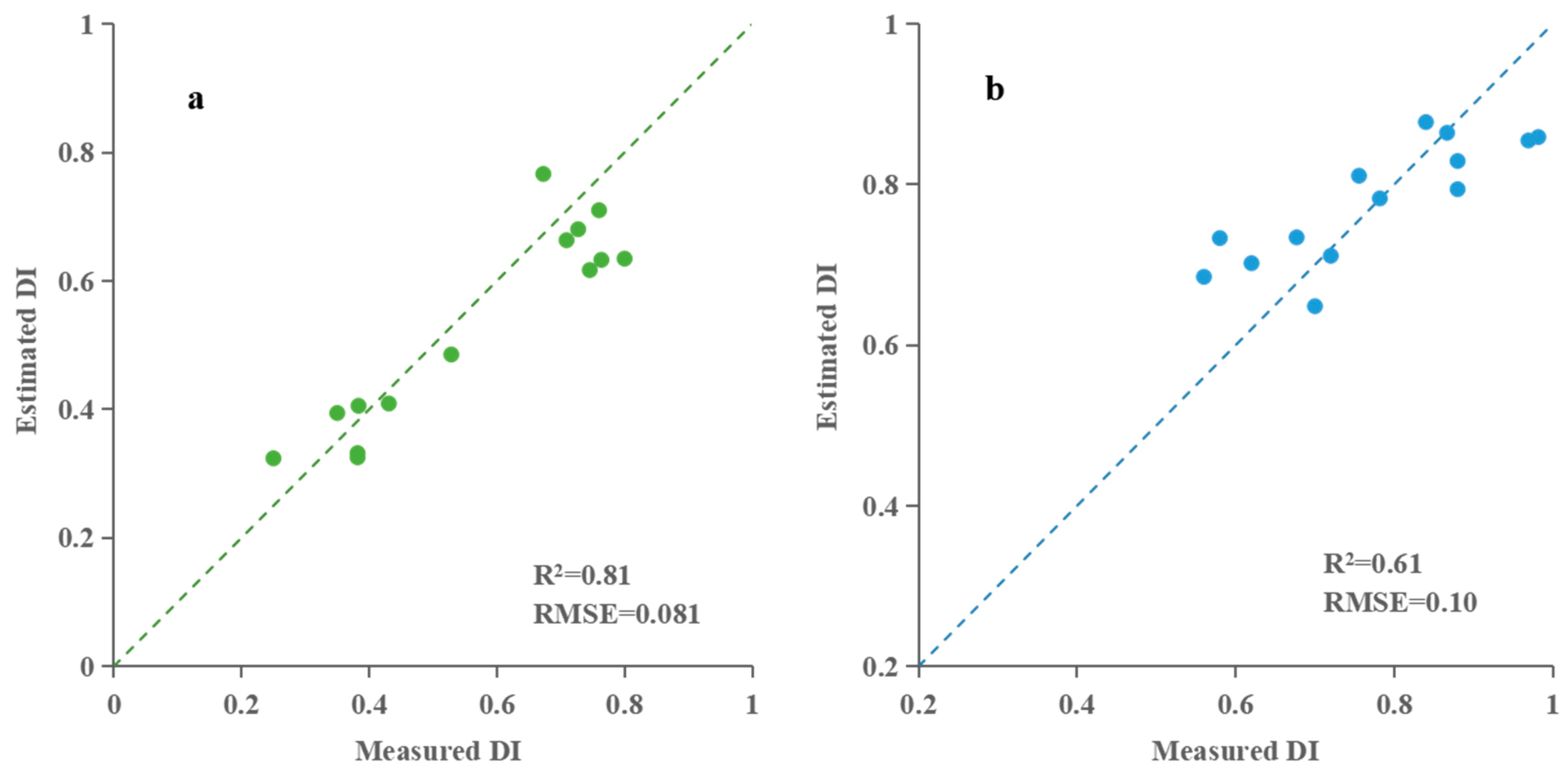
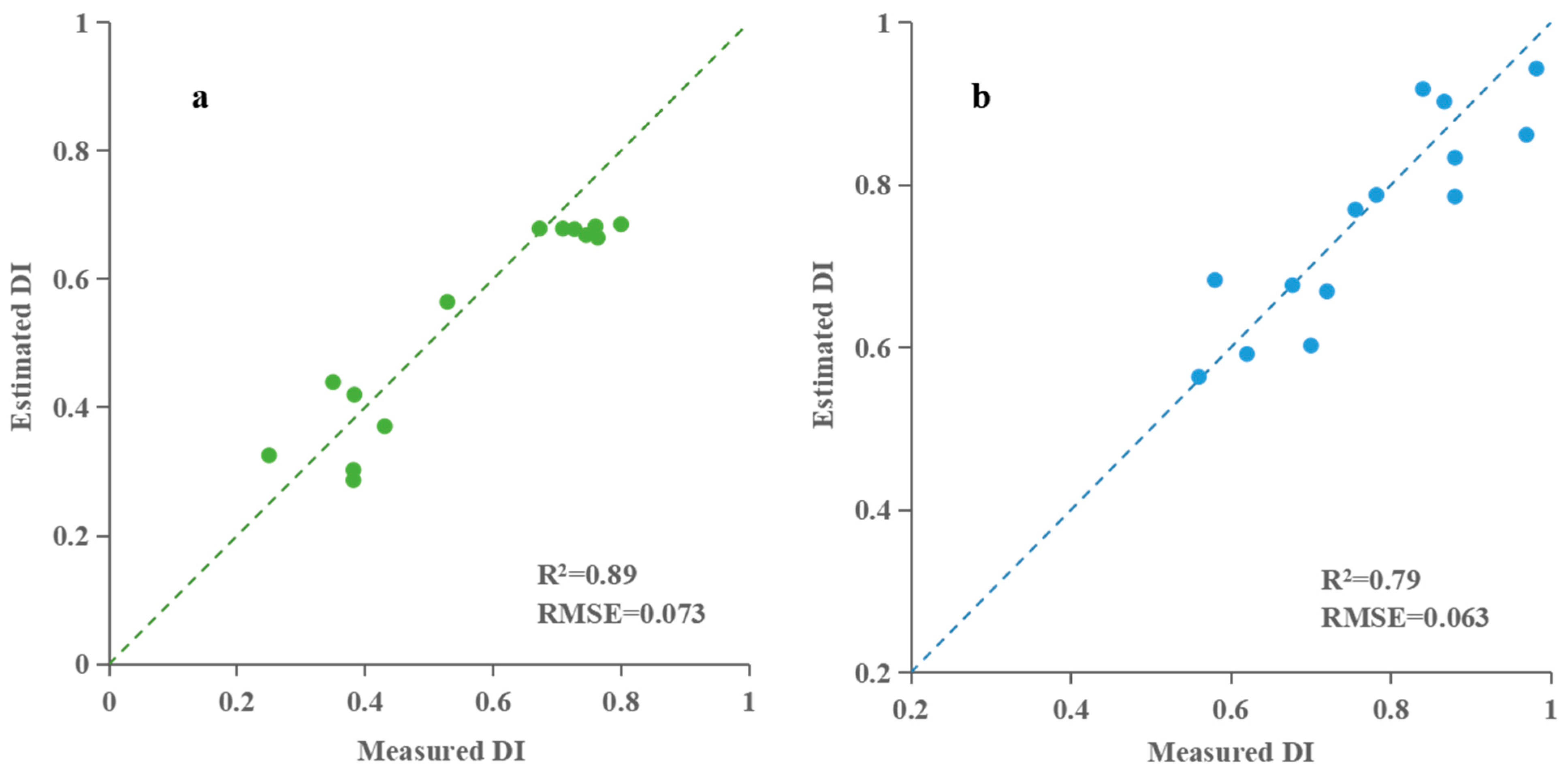
| Growth Stage | Parameter Type | Model | Training Set | Validation Set | ||
|---|---|---|---|---|---|---|
| R2 | RMSE | R2 | RMSE | |||
| The early stage of taro formation | Hyperspectral characteristic parameter | PLSR | 0.79 | 0.086 | 0.81 | 0.081 |
| RFR | 0.92 | 0.056 | 0.84 | 0.075 | ||
| BPNN | 0.92 | 0.054 | 0.89 | 0.074 | ||
| Multispectral vegetation index | PLSR | 0.76 | 0.098 | 0.85 | 0.074 | |
| RFR | 0.89 | 0.069 | 0.83 | 0.082 | ||
| BPNN | 0.87 | 0.074 | 0.82 | 0.084 | ||
| The middle stage of taro formation | Hyperspectral characteristic parameter | PLSR | 0.59 | 0.081 | 0.61 | 0.10 |
| RFR | 0.58 | 0.088 | 0.62 | 0.096 | ||
| BPNN | 0.90 | 0.042 | 0.79 | 0.063 | ||
| Multispectral vegetation indices | PLSR | 0.49 | 0.11 | 0.45 | 0.11 | |
| RFR | 0.83 | 0.074 | 0.74 | 0.099 | ||
| BPNN | 0.87 | 0.057 | 0.81 | 0.076 | ||
Disclaimer/Publisher’s Note: The statements, opinions and data contained in all publications are solely those of the individual author(s) and contributor(s) and not of MDPI and/or the editor(s). MDPI and/or the editor(s) disclaim responsibility for any injury to people or property resulting from any ideas, methods, instructions or products referred to in the content. |
© 2025 by the authors. Licensee MDPI, Basel, Switzerland. This article is an open access article distributed under the terms and conditions of the Creative Commons Attribution (CC BY) license (https://creativecommons.org/licenses/by/4.0/).
Share and Cite
Wang, Y.; Chen, Y.; Shu, Z.; Zhu, S.; Zhang, W.; Liu, T.; Sun, C. Integration of UAV Remote Sensing and Machine Learning for Taro Blight Monitoring. Agronomy 2025, 15, 1189. https://doi.org/10.3390/agronomy15051189
Wang Y, Chen Y, Shu Z, Zhu S, Zhang W, Liu T, Sun C. Integration of UAV Remote Sensing and Machine Learning for Taro Blight Monitoring. Agronomy. 2025; 15(5):1189. https://doi.org/10.3390/agronomy15051189
Chicago/Turabian StyleWang, Yushuai, Yuxin Chen, Zhou Shu, Shaolong Zhu, Weijun Zhang, Tao Liu, and Chengming Sun. 2025. "Integration of UAV Remote Sensing and Machine Learning for Taro Blight Monitoring" Agronomy 15, no. 5: 1189. https://doi.org/10.3390/agronomy15051189
APA StyleWang, Y., Chen, Y., Shu, Z., Zhu, S., Zhang, W., Liu, T., & Sun, C. (2025). Integration of UAV Remote Sensing and Machine Learning for Taro Blight Monitoring. Agronomy, 15(5), 1189. https://doi.org/10.3390/agronomy15051189