Article

Spatial and Temporal Variability in Yield Maps Can Localize Field Management—A Case Study with Corn and Soybean

by
Eduardo G. de Souza
1,*,
Raj Khosla
2,
Kenneth A. Sudduth
3,
Jerry A. Johann
4 and
Claudio L. Bazzi
5
1
Laboratory of Agricultural Mechanization and Precision Agriculture (LAMAP), Technological and Exact Sciences Center, State University of West Paraná (UNIOESTE), Cascavel 85819110, PR, Brazil
2
Department of Agronomy, Kansas State University, Manhattan, KS 66506, USA
3
Cropping Systems and Water Quality Research Unit, USDA Agricultural Research Service, Columbia, MO 65211, USA
4
Research Center for Geotechnologies and Data Science, State University of West Paraná (UNIOESTE), Cascavel 85819110, PR, Brazil
5
Multi-user Laboratory of Agro Technologies (AgriLab), Federal University of Technology of Paraná (UTFPR), Medianeira 85722332, PR, Brazil
*
Author to whom correspondence should be addressed.
Agronomy 2025, 15(5), 1179; https://doi.org/10.3390/agronomy15051179
Submission received: 19 March 2025 / Revised: 22 April 2025 / Accepted: 3 May 2025 / Published: 13 May 2025
(This article belongs to the Section Precision and Digital Agriculture)

Abstract

:
Yield maps represent crop production output and are essential for evaluating within-field spatial variability. Managing this yield variability is critical for precision and digital agriculture to facilitate optimized crop yield and reduced environmental impact. This work evaluated the spatial and temporal variability in corn and soybean yield data from three conventionally managed agricultural fields, with nine, three, and four seasons’ data. The data variability was measured through standard deviation (SD) and coefficient of variation (CV%). After separately normalizing each year of the yield data set, the temporal variability (TSD and TCV%) was calculated by grid cell for each field across years. A new index is proposed in this paper, the yield performance index (YPI, the ratio of mean normalized yield ( Y ¯ N ) to the TSD), as an index with a lower value for lower yield and higher temporal variability. Two, three, and four zones were delineated using only YPI. These zones were valuable for identifying areas needing particular attention, with consistently (i) high yields and low variability or (ii) low yields and high variability.

1. Introduction

Issues related to the land are usually expressed with thematic maps (TMs). These employ graphical symbols where a specific geographically referenced phenomenon occurs. Data acquisition, investigation, interpretation, and representation are necessary to create TMs. The TMs facilitate the identification of similarities and enable the visualization of spatial correlations. TMs are usually generated based on measurements of crop, soil, and topography parameters to analyze the variability in these parameters and compare that variability to crop yield [1]. Choropleth maps are a specific case of TMs used in precision agriculture and can be built from categorical data (e.g., elevation) or relative data (e.g., density) [1]. Yield maps, a choropleth map, are an essential tool for evaluating spatial variability in agricultural fields.
Yield mapping delivers crucial information for evaluating crop variability within a field and highlights the importance of combining data from all sources of spatial variability with the farmer’s knowledge [2]. Several years of data collected under different weather conditions can identify problem areas, improve management, and increase yields [3], essential in characterizing spatial and temporal variability. Eghball and Varvel [4] found that corn had significantly less temporal yield variability than soybean (as concluded by [5]) or sorghum, and that the temporal variability was more critical than spatial variability. Jaynes and Colvin [5], using six years of corn and soybean data, also found that the yield structure and spatial pattern vary from year to year.
Yield data from the harvester’s monitoring device usually have considerable variability due to inherent measurement system noise and various operational and calibration conditions. Hence, before generating yield maps, it is essential to preprocess these noisy data using data-filtering techniques [6,7,8,9]. A standardized protocol is often used to analyze and map yield data and delineate management zones (MZs) and can include the generic steps shown in Figure 1 [1]. In each step of the delineation, the method must be decided. The steps selected in this case study are highlighted in blue.
Delineating MZs is critical in optimizing input use and maximizing crop yield in precision agriculture. Several data sources and analytical techniques can delineate sub-regions within a field with a relatively homogeneous combination of yield-limiting factors [10]. Two approaches commonly used for delineating MZs [11] are (i) empirical, which uses the yield frequency distribution and expert knowledge to define delineations [12,13,14,15,16], and (ii) cluster analysis, such as K-means (KM) and Fuzzy C-means (FCM) [11,17,18]. Cluster analysis enables greater differentiation among MZs or yield classes, typically employing stable attributes related to the target variable (e.g., yield); however, empirical methods are simpler and often utilize the target variable directly to delineate MZs [11].
Blackmore et al. [13], using yield from four fields over six years, separated temporal effects into two parts: the inter-year offset, characterized by the median of the yield, and the temporal variance map, showing the spatial changes over time, and concluded that homogenous MZs can be delineated with the spatial and temporal trend maps.
Maestrini and Basso [14] analyzed data from 338 corn, soybean, wheat, and cotton fields in the US Midwest and concluded that yield depended on the interaction between topography and rainfall patterns. They measured the yield spatial variability, the field yield variations within a single year, and the yield temporal variability, with each field variation observed across the years. Yield variability was significantly influenced by the hydrological dynamics associated with waterlogging during moist spring periods and drought conditions that prevail during the summer grain-filling phase. The authors advocated implementing strategic management approaches to stabilize yield zones and tactical management methods for unstable areas, leveraging within-season remote sensing observations.
Maestrini and Basso [15] also divided 571 fields planted with corn, cotton, soybean, and wheat in the US Midwest into stable and unstable zones and concluded that previous years’ yield maps best predicted spatial variability in the stable zones since the stable component of yield spatial distribution depended primarily on soil properties and landscape. Nevertheless, the yield spatial variability in the unstable zones was more related to the interaction between soil characteristics, landscape, and weather. In both studies, the temporal variability was defined as the standard deviation (SD) across years of the normalized yield. The yield was normalized for each field-year yield map to a zero-arithmetic mean and an SD of 1. Subsequently, for each pixel across all fields, we computed the SD of the normalized yield utilizing all available years pertinent to that specific field. Cells were categorized as unstable if their temporal variability exceeded one and conversely classified as stable if it did not. According to Kharel et al. [16], spatial and temporal variability should be considered when delineating MZs since both were uncorrelated after yield data were analyzed in 847 fields (six farms).
Along with analyzing the spatial and temporal behavior of field attributes, it is also important to locate field areas that require particular attention; various variables and methods are employed across different studies. These variables often involve visual interpretation, application of expert knowledge, and computational models to identify and prioritize areas of interest. Past reports in the literature use these various variables to de-lineate MZs [11,12,13,14,15,16,17,18]. However, this work looks to develop a new variable, the yield performance index (YPI), that captures crop performance by its yield and the variability by the temporal standard deviation, and that could be used to delineate more efficient MZs.
Given past research findings that spatial and temporal variability are important in defining MZs, this study (1) proposes a new method for analyzing within-field spatial and temporal yield variability using a yield performance index (YPI), (2) delineates homogenous MZs with two, three, and four classes, and (3) demonstrates the method using data from two fields in the US and one in Brazil.

2. Materials and Methods

2.1. Study Sites and Data Sets

Data from two agricultural fields (A and B) located in the United States and one (C) located in Brazil (Figure 2, Table 1) were used in the analysis. The equipment used to collect the yield in each experimental field is described in Table 2. The AgDataBox platform (http://adb.md.utfpr.edu.br/map/login, accessed on 10 June 2024) [19] was utilized for data normalization, interpolation, and the creation of yield maps. Data from Field A have been previously reported by Kitchen et al. [20].
Field A is a claypan (silty clay loam) soil field, typically farmed in a corn–soybean rotation, except for the soybean following soybean sequence observed in 1998–1999 and 2003–2004. This soil features a subsoil argillic horizon with a clay content exceeding 500 g kg−1, comprising clays with high shrink–swell properties, specifically, smectitic clay minerals. These clays impart a distinct hydrological attribute, characterized by slow water flow within the soil matrix of the clay layer during wet periods (such as winter and spring) but swift preferential flow through cracks once the profile dries out (during late summer and early fall) [20,21]. The field was managed with no tillage; the mean field slope is 1.8%.
Field B is a portion of a field under a pivot irrigation system. The soil type is a Kim Loam, classified as fine-loamy, mixed, active, mesic Ustic Torriorthents [22], and the texture is a sandy clay loam. The field slope is 0.9% in a single-plane gradient. This field has been managed in a conventional tillage continuous corn cropping system since 1990.
Field C has been cultivated in a no-tillage system since 2000, with a sequence of soybean, wheat, oats, and corn. The soil is classified as Rhodic Ferralsol [23]. The average field slope was 1.2%, ranging from 0.0 to 10.1%. Since this area features several curved contour lines, irregular sampling grids were employed, and the sampling points were positioned in locations that did not align with the curves. Thus, the sampling points were located on the imaginary central line between the elevation contour lines, and field operations were also conducted along these curves.

2.2. Protocol of Data Analysis

In this case study, the steps selected for data analysis, the creation of the TMs, and the delineation of MZs are highlighted in sky blue in Figure 1 (adapted from [1]). The reasons for the selections are described in Section 2.3.1, Section 2.3.3, and Section 2.3.4.

2.3. Exploratory Data Analysis

The exploratory data analysis calculated the mean, median, SD, coefficient of variation (CV%), and normality (the Kolmogorov–Smirnov test at 0.05 significance level). Outliers, or values outside the mean ± 3 SD, were removed [24]. The data variability was measured through SD and CV%. The weighted standard deviation (WSSD, Equation (A1)) was used to calculate the SD when comparing yield data with different numbers of measurements. The classification proposed by Pimentel-Gomes and Garcia [25] was used to classify CV% ≤ 10% as low, 10% < CV% ≤ 20% as medium, 20% < CV% ≤ 30% as high, and CV% > 30% as very high.

2.3.1. Data Normalization and Creation of Choropleth Maps

The yield values were normalized ( Y N ) using the mean method (Equation (1)) [2,20,26] to stabilize these data, which are often heavily influenced by variations in climate and precipitation. Then, since there is more than one year of yield data for each field, the arithmetic mean of the normalized yield was calculated, generating a single variable corresponding to the mean normalized yield ( Y ¯ N ). After that, yield choropleth maps (Figure 1 (step 3)) were created to evaluate the yield distribution visually.
Y N i = Y i Y ¯ ,
where Y N i —normalized yield at point i; Y i —yield at point i; Y ¯ —mean yield for the specific year.

2.3.2. Yield Performance Index

The yield performance index (YPI) (Equation (2)) was introduced to identify places in the field that may require particular management attention. If YPI is low, it indicates a low yield and high temporal variability; if YPI is high, it signifies a high yield and low temporal variability.
Y P I i = Y ¯ N i T S D i ,
where Y ¯ N i —mean normalized yield at the point i; T S D i —temporal standard deviation at the point i.

2.3.3. Data Interpolation

The data of Y ¯ N , TSD, and YPI were interpolated to create continuous and smooth TMs and MZs. The Inverse Distance Weighted (IDW) interpolation was used, as the number of data pairs exceeded 300, the maximum allowed by ADB-Map for kriging. The choice of IDW should not be a problem because when dealing with large sample sizes (from 455 to 1585 data points), the choice between IDW interpolation and kriging becomes less critical [27]. Using the interpolation selection index (ISI, Equation (A2)) [19], the best exponent and number of neighbors for IDW were found. Grids of 4 × 4 m (Field B), 6 × 6 m (Field C), and 8 × 8 m (Field A) were created to increase the density of points and facilitate the delineation of smoother and more continuous TMs. The ADB-Map automatically sets the pixel size as 1/100 of the larger dimension in the eastern/western direction [19].
The SD and CV% were calculated for the mean normalized yield ( Y ¯ N ) of each data set, corresponding to the spatial variability (SSD, Equation (3) and SCV%, Equation (4)):
S S D = i = 1 n Y ¯ N i Y ¯ N ¯ 2 n 1 ,
S C V % = 100 S S D Y ¯ N ¯   ,
where SSD—yield spatial standard deviation; SCV—yield spatial coefficient of variation; Y ¯ N i —mean normalized yield at point i; Y ¯ N ¯ —mean of mean normalized yield ( Y ¯ N ).
The temporal variability (TSD, Equation (5) and TCV%, Equation (6)) was calculated across each grid cell of interpolated normalized yield ( Y N ) of each year and for each field [16].
T S D i = i = 1 n Y N i j Y ¯ N i 2 n 1
T C V % i = 100 T S D i Y ¯ N i ,
where TSDi—yield temporal standard deviation of yield i; T C V % i —yield temporal coefficient of variation i; Y N i j —mean normalized yield at point i; Y ¯ N i —mean normalized yield at point i

2.3.4. Data Clustering, Rectification, and Evaluation of the Management Zones

To account for spatial and temporal variability when delineating MZs [16], we selected YPI as the input variable. Cluster analysis was chosen because it is superior to empirical classification. The FCM clustering algorithm was selected because it is powerful and flexible, but it may not always be the best choice for every situation. Its most notable feature is the adaptability of its membership, which can result in more refined clustering outcomes in contrast to rigid clustering techniques such as K-means, where each data point is assigned to only a single cluster [28]. The FCM algorithm delineated two, three, and four zones, building upon previously interpolated YPI. The rectification of the MZs was performed using the algorithms proposed by Betzek et al. [19] to remove isolated pixels and small regions. The median method, square kernel format, and 5 × 5 kernel sizes were used.
The delineated MZs were evaluated (see Appendix A for details and equations) using:
(i)
Analysis of variance (ANOVA) using the Tukey test at 0.05% significance to identify whether sub-regions within the MZs designed show significant differences in the mean value of the variable of interest;
(ii)
Variance Reduction (VR%) [19]: measures the reduction in the sum of the MZs data variances;
(iii)
Fuzziness Performance Index (FPI) [29]: evaluates the degree of fuzziness in a classification;
(iv)
Modified Partition Entropy (MPE) [29]: evaluates the uncertainty in cluster assignments;
(v)
Improved Cluster Validation Index (ICVI) [19]: a combination of the FPI, MPE, and VR%;
(vi)
Smoothness Index (SI%) [19]: characterizes the smoothness of the boundary curves of MZs;
(vii)
Fragmentation index (FI%) [19]: characterizes the division of land into smaller, often irregularly shaped parcels, which can impact land management strategies;
(viii)
Global Quality Index (GQI) [1]: it looks to find the optimum number of classes during MZ delineation, considering all indices together.
The definition of the number of MZs was conducted in two stages:
(i)
ANOVA: This procedure was performed to verify if the mean values of the YPI (target variable) in each class were statistically distinct [19] using Tukey’s range test (0.05 level).
(ii)
Choosing the best GQI (the lowest), which contains all the remaining ones (FPI, MPE, VR%, ICVI, SI%, and FI%).

3. Results

3.1. Summary Statistics

Descriptive statistics of the original yield data for nine (Field A), three (Field B), or four years (Field C) are shown in Table 3. Among all three fields, we observed (Table 3) that:
  • The 2003 soybean in Field A, 2002 corn in Field A, 2012 corn in Field B, and 2012 soybean in Field C presented very high SCV% (>30%);
  • Notably, low minimum yield values were seen for the 1999 soybean in Field A, the 2003 soybean in Field A, and the 2002 corn in Field B;
  • The highest weighted spatial variability (WSCV%) was found for corn in Field A (26.3%) and the lowest for soybeans in Field A (17.5%).
Table 3. Summary of descriptive statistics calculated for the original yield data without outliers for each year and field under consideration.
FieldYear/CropOriginal Yield (Sampling Data) (t ha−1)SSDSCV%WSSDWSCV%
Soybean or CornMeanSoybean or CornMean
No.SMin.MeanMedianMax.(t ha−1)(%)(t ha−1)(%)
A1996 Soybean12091.803.073.104.320.4113.30.410.8717.524.0
1998 Soybean12071.592.532.573.250.3012.0
1999 Soybean12130.291.391.362.660.4229.9
2001 Soybean12021.282.492.503.670.3815.3
2003 Soybean *12160.261.551.572.950.4931.6
2004 Soybean11921.462.942.994.090.4314.6
1997 Corn12161.176.416.5611.851.9029.61.4026.3
2000 Corn11916.319.279.3911.420.859.2
2002 Corn12120.063.063.116.731.2340.2
B2011 Corn4556.599.289.4411.420.909.71.6019.7
2012 Corn4550.866.336.6710.782.0732.7
2013 Corn4544.638.859.3511.721.6118.2
C2012 Soybean15850.632.582.464.820.9637.10.6718.1
2013 Soybean15752.124.154.146.130.6615.9
2015 Soybean *15723.244.724.716.130.4710.0
2016 Soybean15662.003.453.415.020.4914.1
No.S: number of samples; Min.: minimum; Max.: maximum; SSD: spatial standard deviation; WSSD: weighted SSD; SCV%: spatial coefficient of variation; WSCV%: weighted SCV%. * normally distributed by the Kolmogorov–Smirnov test at a 0.05 significance level.

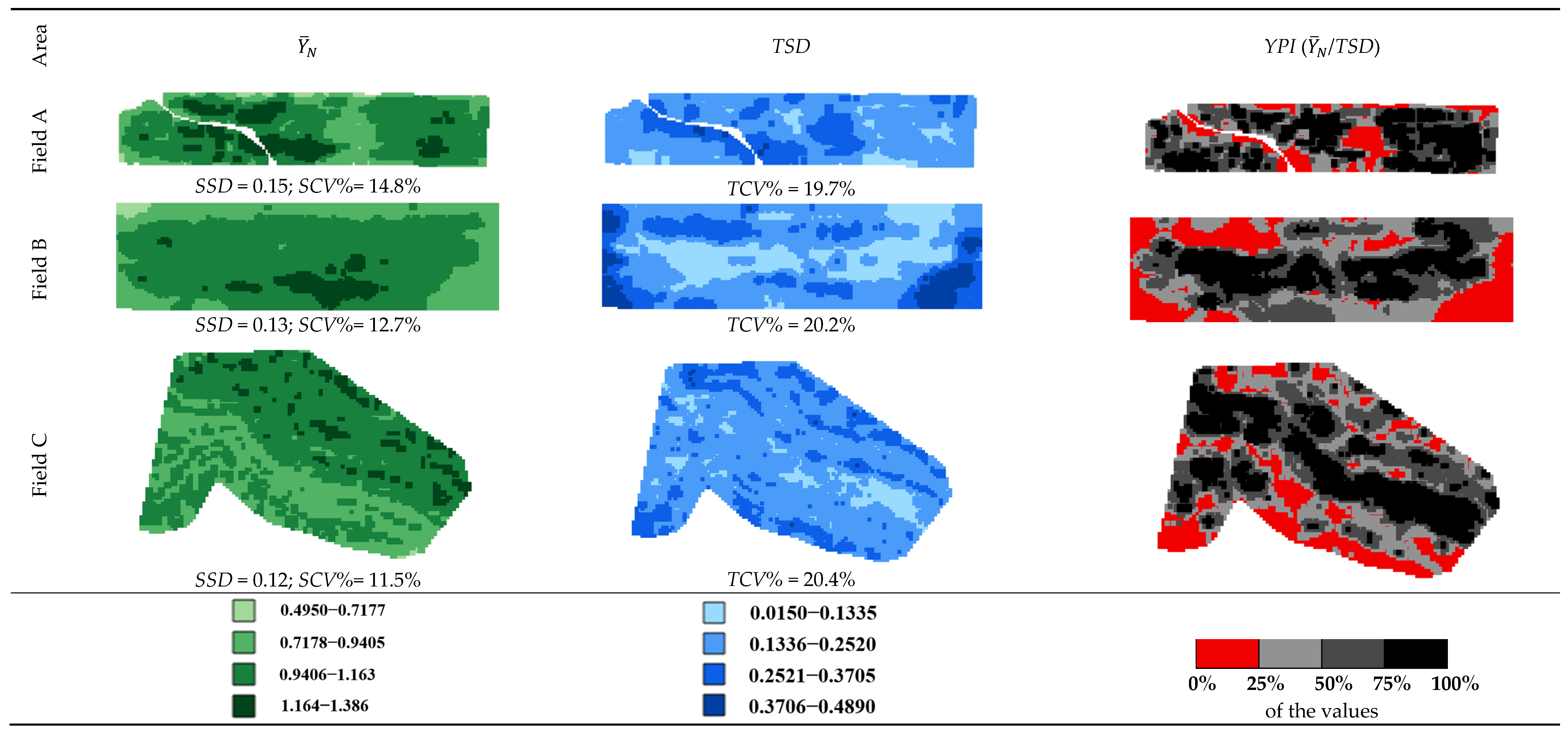
3.2. Yield, Temporal Variability, and Yield Performance Index Maps

Figure 3 shows the thematic maps of (i) the mean normalized yields ( Y ¯ N ), (ii) the temporal standard deviation (TSD), and (iii) the yield performance index (YPI) for each field. To improve readability, the maps of Y ¯ N and TSD were classified by manual intervals and YPI by quantiles because the data range was similar for the first two variables and not for the third. Planting and other farm operations were conducted in the east–west direction for Fields A and B, whereas operations in Field C were performed along level curves (i.e., contour farming). A headland yield reduction was observed for Fields A and B, as shown by the red regions of YPI (Figure 3). This reduction was absent in Field C because a 15 m strip was discarded in the east and west parts. The yield pattern in Field C was concordant with the elevation contour lines. The data normalization enabled a 37% reduction in spatial data variability (Table 3 and Table 4).
The Y ¯ N distribution shows a yield increase from the border to the center for Fields A and B and from the south to the north of Field C. For the data variability measured by the TSD, it increased like Y ¯ N , i.e., from the border to the center for Field A and inversely for Fields B and C. And finally, the YPI ( Y ¯ N / T S D ) increased from the border to the center for Fields B and C, and it is almost uniformly distributed across Field A. In summary, all three variables ( Y ¯ N , TSD, and YPI) have distinct behaviors.
The mean normalized yield spatial variability (SCV%, Figure 3, Table 4) of Field A was the highest (15%), and of Field C, the lowest (12%). Furthermore, all fields’ mean normalized yield temporal variability (TCV%) was about 20%.

3.3. Management Zones

Although the thematic maps of YPI can show their spatial variability, visualization of the MZs is also helpful because this makes it possible to delineate statistically distinct classes [19]. Using the YPI of each field (A, B, and C), MZs were delineated (Table 5, Figure 4) with two, three, and four classes. The similarity between the MZs with four zones and the YPI quantile classification (Figure 3) was remarkable. Evaluation of the quality of the MZs was conducted in two stages, conforming to item 2.3.4: First, it was found that all delineated classes were statistically different. Second, after analysis of the GQI index (the lower, the better), it was found that four, two, and four classes were the optimum number of classes (NC) in Fields A, B, and C, respectively.
We highlight that the choice of the best NC using only one of the MZ quality indices FPI, MPE, VR%, ICVI, SI%, and FI% (the lower the FPI, MPE, ICVI, and FI%, the better; however, the opposite occurs with VR% and SI%) (Appendix A) could lead to controversial results; let us examine the case of Field C: (i) the indices FPI, ICVI, and SI%, and FI% would indicate two classes; (ii) the VR%, three, and (iii) the MPE, ICVI, and FI%, four. These discrepancies highlight the importance of using the combined GQI index.

4. Discussion

It was found that the weighted spatial yield variability (WSCV%) for corn in rainfed Field A was 26%, considerably higher than in irrigated Field B (20%) (Table 3). The WSCV% in Field A and Field B for soybeans was approximately 18%, lower than that of the corn fields, corroborating the results from Jaynes and Colvin [5].
Concerning (i) the mean normalized yields ( Y ¯ N ), (ii) the temporal standard deviation (TSD), and (iii) the yield performance index (YPI) of each field (Figure 3), it could be observed that:
  • The highest yields ( Y ¯ N ,   d a r k   a n d   v e r y   d a r k   g r e e n ) correspond to regions that could benefit from a differentiated treatment that takes advantage of their high productive potential. However, these regions do not always correspond to low TSD (blue maps in Figure 3), so temporal yield stability must be considered before implementing a treatment plan.
  • The large part of the area with higher TSD coincides with low Y ¯ N . Although corn and soybean were planted in these fields in rotation, the time-dependent variations in normalized yield may be due to plant growth response to heat, precipitation, soil water, and plant nitrogen availability. Reducing TSD is a challenge that can be effectively achieved through precision agriculture, soil conservation practices, crop rotation, and advanced data analysis techniques, as remarked by Yost et al. [30].
  • The information presented in the YPI shows the ratio of mean normalized yield ( Y ¯ N ) to the TSD, having two particular cases: (i) the black areas correspond to consistently high yields with low variability; (ii) the red areas have low yields with high variability. This information is more visible than when presented separately as Y ¯ N and TSD and can help define parts of the field that should receive particular attention.
The descriptive statistics of the mean normalized yield ( Y ¯ N , Table 4) for each field showed that the temporal variability (20%) was larger than the spatial within-field variability (13%) in all fields (Table 4), with a mean of 57%, corroborating what Eghbal and Varvel [4] and Maestrini and Basso [14] observed.
During the MZ delineation, the ideal number of classes was found to be four, two, and four for Fields A, B, and C, respectively. It has been demonstrated that the YPI spatial dependence is sufficiently large to delineate MZs, allowing for the implementation of differential management practices. This implementation of MZs in the field holds significant potential for optimizing economic returns while minimizing environmental impacts. However, dividing the field into four classes may introduce complications for management operations. Therefore, it may be more practical to adopt two classes in all fields.
It is essential to recognize that many factors that have not been considered might have contributed to the observed Y ¯ N , TSD, and YPI patterns, like geomorphology, soil chemical and physical attributes, and crop coverage [31]. Nonetheless, the variable YPI has the advantage of presenting temporal integration, multi-crop capability, and a more straightforward interpretation.
A more detailed comparison with previous studies was impossible because the YPI index was initially proposed in this work.

5. Conclusions

The spatial and temporal variability in yield data from three conventional agriculture fields were analyzed. The mean normalized yield spatial variability (SCV) varied from 12 to 15%, and the mean normalized yield temporal variability (TCV) was about 20% for all fields. Typically, crop harvests with a high SCV were associated with low yields. That reinforces the potential of precision agriculture to improve yield averages by reducing field variability with site-specific management. Furthermore, the yield performance index (YPI) delineated four, two, and four management zones (MZs) in Fields A, B, and C, respectively, proving helpful in identifying areas that require particular attention, characterized by consistently high yields and low variability, or low yields and high variability. Furthermore, these MZs help enable variable-rate fertilizer application.
Further research is needed with more years of data, testing YPI in diverse environments and integrating specific soil/climate data layers. Studying the influence of climatic and management factors, as well as topographic, soil, and plant properties, on the spatial and temporal variability in yield maps would also be beneficial.

Author Contributions

Conceptualization, C.L.B., E.G.d.S., K.A.S. and R.K.; data curation, E.G.d.S.; formal analysis, C.L.B., E.G.d.S. and J.A.J.; investigation, E.G.d.S., K.A.S. and R.K.; methodology, E.G.d.S., J.A.J., K.A.S. and R.K.; writing—original draft, E.G.d.S.; writing—review and editing, C.L.B., E.G.d.S., J.A.J., K.A.S. and R.K. All authors have read and agreed to the published version of the manuscript.

Funding

This research received no external funding.

Data Availability Statement

The data sets presented in this article are not readily available because they are proprietary.

Acknowledgments

The authors would like to thank the Western Paraná State University (UNIOESTE), the Federal University of Technology of Paraná (UTFPR), the Coordination for the Improvement of Higher Education Personnel—Brazil (CAPES)—Finance Code 001, and the National Council for Scientific and Technological Development (CNPq). We also thank Eng. Aldo Tasca for making his property available. The authors want to acknowledge the support provided by the Agricultural Experiment Station at Colorado State University, as well as Kansas State Research and Extension.

Conflicts of Interest

The authors declare no conflicts of interest.

Abbreviations

AcronymDescription
ASCAverage Silhouette Coefficient
CV%Coefficient of Variation
FI%Fragmentation index
FPIFuzziness Performance Index
GAGlobal Accuracy
GQIGlobal Quality Index
ICVIImproved Cluster Validation Index
IDWInverse Distance Weighted Interpolation
KappaKappa Coefficient
MGQIModified Global Quality Index
MPEModified Partition Entropy
Y ¯ Mean Yield
Y ¯ N Mean Normalized Yield
Y ¯ N ¯
MZ
Mean of Mean Normalized Yield
Management Zone
NC
SCV%
Number of classes
Spatial Coefficient of Variation;
SDStandard Deviation
SI%Smoothness Index
SSDSpatial Standard Deviation;
TCV%Temporal Coefficient of Variation
TMThematic Map
TSDTemporal Standard Deviation
VR%Variance Reduction
WSSDWeighted Standard Deviation
YYield
Y ¯ N Normalized Yield
YPIYield Performance Index

Appendix A

Appendix A.1. The Weighted Standard Deviation

The weighted standard deviation (WSSD, Equation (A1)) was used to calculate the SD when comparing yield data with a different number of measurements.
W S S D = i = 1 M N i 1   ×   S S D i 2 ( i = 1 M N i   ) M
where Ni is the number of observations in each crop year; M is the number of crop years; SSDi is the yield standard deviation in the crop year i.

Appendix A.2. The Interpolation Selection Index

Bier and Souza proposed the interpolation selection index (ISI, Equation (A2); [19]).
I S I = A B S ( A E ) max j i = 1 A B S ( A E ) + S A E min j i = 1 S A E max j i = 1 A B S S A E
where ISI is the interpolation selection index; AE is the average error; SAE is the standard deviation of the average error; A B S A E is the absolute value of the average error of the crossed validation; m i n | i = 1 j is the lowest value found between the compared j models; m a x | i = 1 j is the highest value found between the compared j models.

Appendix A.3. Evaluation Indices of Management Zones’ Quality

1. Variance Reduction (VR%) [19] (Equation (A3)): is calculated for the target variable, with the expectation that the sum of the variances in the data from MZs generated is smaller than the total variance:
V R % = 1 i = 1 c W i × V m z i V f i e l d × 100
where c is the number of MZs; Wi is the proportion of the area of i-th MZ to the total area; Vmzi is the data variance of the i-th MZ; and Vfield is the field data variance. The greater, the better.
2. Fuzziness Performance Index (FPI) [29] (Equation (A4)): the degree of separation between the fuzzy c groups generated from a data set. FPI varies between 0 and 1. The lower, the better.
F P I = 1 c ( c 1 ) 1 j = 1 n i = 1 c ( m i j ) 2 / n
where c is the number of groups; n is the number of elements in the data set; and mij is the element of the fuzzy pertinence matrix M.
3. Modified Partition Entropy (MPE) [29] (Equation (A5)): estimates the difficulty level of the organization of c groups. The lower, the better.
M P E = j = 1 n i = 1 c m i j   l o g   ( m i j ) / n l o g   c
where c is the number of groups; n is the number of elements in the data set; and mij is the element of the fuzzy pertinence matrix M.
4. Improved Cluster Validation Index (ICVI) [19] (Equation (A6)): addresses a potential issue when the FPI, MPE, and VR% estimates do not indicate similar methods. The lower, the better.
I C V I i = 1 3 × F P I i M a x F P I + M P E i M a x M P E + 1 V R % i M a x V R %
where FPIi is the FPI value of the i-th variable selection method; MPEi is the MPE value of the i-th variable selection method; VR%i is the VR% value of the i-th variable selection method; and Max{Index_X} represents the maximum value of the Index_X among the n variable selection methods.
5. Smoothness Index (SI%) [19] (Equation (A7)): The closer to 100%, the better.
S I % = 100 i = 1 k N M H i 4 P H + j = 1 k N M V j 4 P V + l = 1 k N M D d l 4 P D d + m = 1 k N M D e m 4 P D e × 100
where N M H i is the number of changes in row i (horizontal); N M V j is the number of changes in column j (vertical); N M r D l is the number of changes in diagonal l (right diagonal r D ); N M D e m is the number of changes in diagonal m (left diagonal D e ); k is the maximum number of pixels in a row, column, or diagonal; P H is the possibility of changes in horizontal pixels; P V is the possibility of changes in vertical pixels; P D d is the possibility of changes in the right diagonal D d ; P D e is the possibility of changes in the left diagonal D e .
6. Fragmentation index (FI%) [19] (Equation (A8)): This index considers the ratio of the number of zones (NMZ) to the number of classes (NC). The higher the FI%, the higher the fragmentation.
F I % = 100 N M Z N C N C
7. Global Quality Index (GQI) [1] (Equation (A9)): it looks to find the optimum number of classes during MZs delineation, taking into account the values of ICVI, FIr%, and SIr%:
G Q I i = I C V I i × ( 100 + F I r % i ) S I r % i
where r means rectified value.

References

  1. Aikes, J., Jr.; Souza, E.G.; Bazzi, C.L.; Sobjak, R. Thematic Maps and Management Zones for Precision Agriculture: Systematic Literature Study, Protocols, and Practical Cases; Poncã: Curitiba, Brazil, 2021. [Google Scholar]
  2. Stafford, J.; Ambler, B.; Lark, R.; Catt, J. Mapping and interpreting the yield variation in cereal crops. Comput. Electron. Agric. 1996, 14, 101–119. [Google Scholar] [CrossRef]
  3. Pennington, D. The Importance of Collecting Accurate Yield Monitoring Data. Michigan State University Extension. 2016. Available online: https://www.no-tillfarmer.com/articles/6103-the-importance-of-collecting-accurate-yield-monitoring-data (accessed on 14 January 2025).
  4. Eghball, B.; Varvel, G.E. Fractal analysis of temporal yield variability of crop sequences: Implications for site-specific management. Agron. J. 1997, 89, 851–855. [Google Scholar] [CrossRef]
  5. Jaynes, D.B.; Colvin, T.S. Spatiotemporal variability of corn and soybean yield. Agron. J. 1997, 89, 30–37. [Google Scholar] [CrossRef]
  6. Robinson, T.; Metternicht, G. Comparing the performance of techniques to improve the quality of yield maps. Agric. Syst. 2005, 85, 19–41. [Google Scholar] [CrossRef]
  7. Sudduth, K.A.; Drummond, S.T. Yield editor: Software for removing errors from crop yield maps. Agron. J. 2007, 99, 1471–1482. [Google Scholar] [CrossRef]
  8. Lyle, G.; Bryan, B.A.; Ostendorf, B. Post-processing methods to eliminate erroneous grain yield measurements: Review and directions for future development. Precis. Agric. 2013, 15, 377–402. [Google Scholar] [CrossRef]
  9. Sun, W.; Whelan, B.; McBratney, A.B.; Minasny, B. An integrated framework for software to provide yield data cleaning and estimation of an opportunity index for site-specific crop management. Precis. Agric. 2013, 14, 376–391. [Google Scholar] [CrossRef]
  10. Moharana, P.C.; Jena, R.K.; Pradhan, U.K.; Nogiya, M.; Tailor, B.L.; Singh, R.S.; Singh, S.K. Geostatistical and fuzzy clustering approach for delineation of site-specific management zones and yield-limiting factors in irrigated hot arid environment of India. Precis. Agric. 2020, 21, 426–448. [Google Scholar] [CrossRef]
  11. Li, X.; Pan, Y.-C.; Ge, Z.-Q.; Zhao, C.-J. Delineation and scale effect of precision agriculture management zones using yield monitor data over four years. Agric. Sci. China 2007, 6, 180–188. [Google Scholar] [CrossRef]
  12. Blackmore, S. The interpretation of trends from multiple yield maps. Comput. Electron. Agric. 2000, 26, 37–51. [Google Scholar] [CrossRef]
  13. Blackmore, S.; Godwin, R.J.; Fountas, S. The analysis of spatial and temporal trends in yield map data over six years. Biosyst. Eng. 2003, 84, 455–466. [Google Scholar] [CrossRef]
  14. Maestrini, B.; Basso, B. Drivers of within-field spatial and temporal variability of crop yield across the US Midwest. Sci. Rep. 2018, 8, 14833. [Google Scholar] [CrossRef] [PubMed]
  15. Maestrini, B.; Basso, B. Predicting spatial patterns of within-field crop yield variability. Field Crops Res. 2018, 219, 106–112. [Google Scholar] [CrossRef]
  16. Kharel, T.P.; Maresma, A.; Czymmek, K.J.; Oware, E.K.; Ketterings, Q.M. Combining spatial and temporal corn silage yield variability for management zone development. Agron. J. 2019, 111, 2703–2711. [Google Scholar] [CrossRef]
  17. Taylor, J.; Wood, G.; Earl, R.; Godwin, R. Soil factors and their influence on within-field crop variability, part II: Spatial analysis and determination of management zones. Biosyst. Eng. 2003, 84, 441–453. [Google Scholar] [CrossRef]
  18. Li, Y.; Shi, Z.; Li, F.; Li, H.-Y. Delineation of site-specific management zones using fuzzy clustering analysis in a coastal saline land. Comput. Electron. Agric. 2007, 56, 174–186. [Google Scholar] [CrossRef]
  19. Sobjak, R.; de Souza, E.G.; Bazzi, C.L.; Schenatto, K.; Betzek, N.M.; Gavioli, A. Incorporation of computational routines in a microservice architecture in AgDataBox platform. Sustain. Comput. Informatics Syst. 2024, 44, 101038. [Google Scholar] [CrossRef]
  20. Kitchen, N.; Sudduth, K.; Myers, D.; Drummond, S.; Hong, S. Delineating productivity zones on claypan soil fields using apparent soil electrical conductivity. Comput. Electron. Agric. 2005, 46, 285–308. [Google Scholar] [CrossRef]
  21. Jamison, V.C.; Smith, D.D.; Thornton, J.F. Soil and Water Research on a Claypan Soil; USDA-ARS Technical Bulletin 1379; US Government Printing Office: Washington, DC, USA, 1967. [Google Scholar]
  22. Soil Survey Division Staff. Soil Survey Manual; Soil Conservation Service. US. Department of Agriculture Handbook 18; US Department of Agriculture: Washington, DC, USA, 2017. Available online: https://www.nrcs.usda.gov/sites/default/files/2022-09/The-Soil-Survey-Manual.pdf (accessed on 14 July 2024).
  23. Baxter, S. World Reference Base for Soil Resources. World Soil Resources Report 103. Rome: Food and Agriculture Organization of the United Nations (2006), pp. 132. ISBN 92-5-10511-4. Exp. Agric. 2007, 43, 264. [Google Scholar] [CrossRef]
  24. Córdoba, M.A.; Bruno, C.I.; Costa, J.L.; Peralta, N.R.; Balzarini, M.G. Protocol for multivariate homogeneous zone delineation in precision agriculture. Biosyst. Eng. 2016, 143, 95–107. [Google Scholar] [CrossRef]
  25. Pimentel-Gomes, F.; Garcia, G.H. Estatística Aplicada a Experimentos Agronômicos e Florestais. Statistics Applied to Agronomic and Forestry Experiments; Biblioteca de Ciências Agrárias Luiz de Queiroz: Piracicaba, Brazil, 2002; 307p. [Google Scholar]
  26. Molin, J.P. Definição de unidades de Manejo a partir de mapas de produtividade. Definition of management units from productivity maps. Eng. Agrícola 2002, 22, 83–92. [Google Scholar]
  27. Milillo, T.M.; Gardella, J.A., Jr. Spatial Analysis of Time of Flight− Secondary Ion Mass Spectrometric Images by Ordinary Kriging and Inverse Distance Weighted Interpolation Techniques. Anal. Chem. 2008, 80, 4896–4905. [Google Scholar] [CrossRef] [PubMed]
  28. Du, K.L. Clustering: A neural network approach. Neural Netw. 2010, 23, 89–107. [Google Scholar] [CrossRef]
  29. Boydell, B.; McBratney, A.B. Identifying potential within-field management zones from cotton-yield estimates. Precis. Agric. 2002, 3, 9–23. [Google Scholar] [CrossRef]
  30. Yost, M.A.; Kitchen, N.R.; Sudduth, K.A.; Sadler, E.J.; Drummond, S.T.; Volkmann, M.R. Long-term impact of a precision agriculture system on grain crop production. Precis. Agric. 2017, 18, 823–842. [Google Scholar] [CrossRef]
  31. Nawar, S.; Corstanje, R.; Halcro, G.; Mulla, D.; Mouazen, A.M. Delineation of soil management zones for variable-rate fertilization: A review. Adv. Agron. 2017, 143, 175–245. [Google Scholar] [CrossRef]
Figure 1. General schematic workflow of actions when generating thematic maps and delineating management zones (the actions used in this case study are highlighted in sky blue Agronomy 15 01179 i001 ) (adapted from [1]). FPI: Fuzziness Performance Index; MPE: Modified Partition Entropy; VR%: Variance Reduction; ICVI: Improved Cluster Validation Index; ASC: average silhouette coefficient; SI%: Smoothness Index; FI%: Fragmentation index; and GQI: Global Quality Index; MGQI: Modified Global Quality Index; Kappa: Kappa coefficient; GA: Global accuracy.
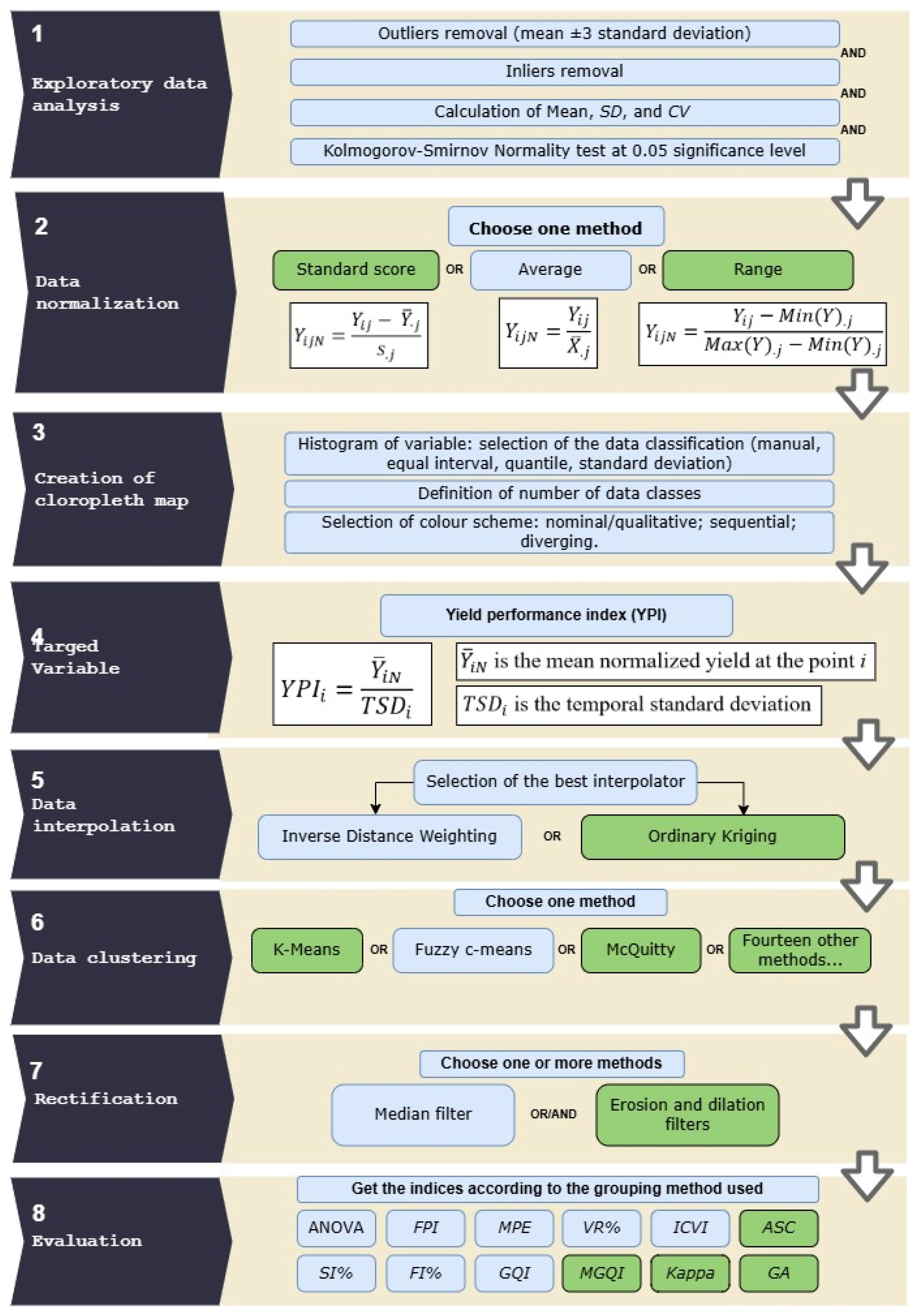
Agronomy 15 01179 g001
Figure 2. Experimental fields A, B, and C visualized using the web platform AgDataBox [19].
Agronomy 15 01179 g002
Figure 3. Thematic maps of mean normalized yields ( Y ¯ N , dimensionless), temporal standard deviation (TSD) of normalized yield, and yield performance index (YPI) for each field (A, B, and C). No data sets were normally distributed. Equal interval classification was used for Y N ¯ and TSD, and quantile classification was used for YPI. Dark colors correspond to higher yields, data variability, and YPI (high yields with low variability).
Agronomy 15 01179 g003
Figure 4. Management zones of yield performance index (YPI) for each field (A, B, and C) using two, three, and four classes. The YPI increases from left to right (C1 to C4). The management zones with the optimum number of classes are highlighted.
Agronomy 15 01179 g004
Table 1. Description of the three experimental fields (A, B, and C) used in the study.
FieldABC
Latitude39.234740.6659−25.1092
Longitude−92.1466−104.9981−53.8319
Area (ha)134.715.6
MunicipalityCentraliaDenverCéu Azul
StateMissouriColoradoParaná
CountryUSUSBR
Soil typeClaypan (Alfisol)Kim LoamRhodic Ferralsol
TillageNo tillageNo tillageNo tillage
Table 2. Equipment used to collect the yield in each experimental field.
CropField AField BField C
YearEquipmentYearEquipmentYearEquipment
Corn Yield97, 00, 02Gleaner R42 combine harvester11, 12, 13Case IH 1660 combine harvester
Soybean Yield96, 98, 99, 01, 03, 04 12, 13, 14, 16Case IH 2388 combine harvester
Gleaner R42 combine harvester (AGCO, Inc., Duluth, GA, USA) with Ag Leader YM2000 yield monitor (AgLeader Technology, Ames, IA, USA); Case IH 1660 combine harvester (CNH Industrial, Basildon, UK) with AgLeader yield monitor; Case IH 2388 harvester with Case AFS PRO 600 yield monitor.
Table 4. Summary of descriptive statistics calculated for the mean normalized yield for each field.
Number Of Crop-YearsMean Normalized Yield  ( Y ¯ N ) SSDSCV%TSVRelation TSV/SSD
(Dimensionless)
FieldNo.SCornSoybeanMin.MeanMedianMax.Range (%)(%)
A1216360.491.001.011.390.890.1514.819.71.33
B4553-0.641.001.021.310.670.1312.720.21.59
C1585-40.691.001.001.290.600.1211.520.41.77
Mean 0.1313.020.11.57
No.S: number of samples; Min.: minimum; Max.: maximum; SSD: spatial standard deviation; SCV%: spatial coefficient of variation.
Table 5. Evaluation of management zones delineated with yield performance index (YPI) for each field (A, B, and C) using two, three, and four classes. NC: number of classes.
Field (Area)NC Tukey’s TestFPIMPEVR%ICVISIr%MZsFIr%GQI
C1C2C3C4
2YPI5.38 a9.37 b 0.0860.10330.70.7394.772502.71
Area (ha)10.392.61
%Area79.9%20.1%
A3YPI4.23 a7.12 b10.6 c 0.0800.08137.40.5890.8123002.56
(13.0 ha) Area (ha)5.137.120.75
%Area39.5%54.8%5.8%
4YPI4.01 a6.77 b10.1 c***0.0780.06938.30.5389.9163002.34
Area (ha)4.277.521.22
%Area32.8%57.8%9.4%
2YPI9.14 a110 b 0.0110.01329.80.3099.6200.30
Area (ha)4.700.042
%Area99.1%0.9%
B3YPI6.14 a23.4 b129 c 0.0460.04748.40.6695.761001.37
(4.7 ha) Area (ha)3.860.840.031
%Area81.5%17.8%0.7%
4YPI5.17 a16.9 b41.1 c153 d0.0480.04349.00.6494.56501.01
Area (ha)3.341.220.160.021
%Area70.5%25.7%3.3%0.4%
2YPI5.17 a9.53 b 0.0650.07917.80.66 ¥95.3104003.46
Area (ha)12.433.18
%Area79.6%20.4%
C3YPI4.79 a7.47 b12.8 c 0.0750.07520.10.65 ¥92.1133333.06
(15.6 ha) Area (ha)9.475.510.63
%Area60.7%35.3%4.0%
4YPI4.55 a6.69 b 9.48 c11.6 d0.0740.06617.80.65 ¥90.0132252.33
Area (ha)7.566.061.620.37
%Area48.5%38.8%10.3%2.4%
NC: Number of classes; C1…C4: class 1 to 4; Sym: Symbology; MZ_A_2: management zones of Field A with 2 zones; FPI: Fuzziness Performance Index; MPE: Modified Partition Entropy; VR%: Variance Reduction; ICVI: Improved Cluster Validation Index; SIr%: Smoothness index rectified; FIr%: Fragmentation index rectified; GQI: Global Quality Index; means followed by the same letter in the same row do not differ statistically among themselves by Tukey’s test (p < 0.05); the best index for each normalization method is highlighted in blue (simple index) and pink (composite index); ¥: indices not statistically different; ***: After the rectification, this class disappeared. The YPI increases from the left (C1) to the right (C4).
Disclaimer/Publisher’s Note: The statements, opinions and data contained in all publications are solely those of the individual author(s) and contributor(s) and not of MDPI and/or the editor(s). MDPI and/or the editor(s) disclaim responsibility for any injury to people or property resulting from any ideas, methods, instructions or products referred to in the content.

