Cropland Expansion Masks Ecological Degradation: The Unsustainable Greening of China’s Drylands

Abstract

In recent years, China’s “greening” trend has drawn great attention. However, does this truly represent ecological improvement? This study aims to figure it out on the mountain–oasis–desert ecosystem in the rid region of Northwest China. By first exploring the vegetation changes and the influence of climate factors and human activities on these changes, we then assessed the regional ecological quality using a combination of the Remote Sensing Ecological Index (RSEI) and the InVEST Habitat Quality Model. The results revealed that the NDVI was indeed increased, but the increase was primarily driven by cropland expansion, with significant NDVI and RSEI growth confined to oases. When croplands were excluded, RSEI values dropped substantially, and 20.9% of the region shows noticeable ecological quality deterioration. Remarkably, 75% of areas with improved RSEI ratings are cultivated lands, which concealed the degradation of natural ecosystems. The InVEST model highlights intensified regional degradation, with habitat quality declining and 9.1% of grasslands converted into croplands. Hurst index projections show 47.5% of vegetation faces sustained degradation. Thus, the observed “greening” primarily reflects cropland expansion rather than ecological improvement. Natural ecosystems in mountainous and desert areas face ongoing severe degradation. This research emphasizes the urgent need for arid regions to balance agricultural expansion with ecological conservation.

1. Introduction

Arid regions, which constitute approximately 40% of Earth’s terrestrial area, are home to over 38% of the global population [1]. Arid regions are notably vulnerable within the global ecosystem, highly sensitive to both climate change and human activities [2,3,4]. Over the past half-century, the expansion of arid lands has been a steady consequence of climatic changes. Factors such as global warming, altered precipitation patterns, and the heightened frequency of extreme weather events have imposed additional burdens on these regions [1,5]. As a result, understanding the ecological changes driving mechanisms affecting arid regions on a macro scale, as well as developing strategies for sustainable management and restoration, have emerged as a critical focus within the fields of global ecology and environmental science.

China encompasses a vast expanse of arid regions, with arid and semi-arid zones constituting over one-third of its terrestrial domain [6]. These areas are characterized by severe natural conditions, notably limited precipitation, elevated evaporation, intense wind erosion, and pronounced water scarcity. Such factors render the ecological carrying capacity particularly vulnerable [1,7]. At the same time, increased human activities such as overgrazing, land cultivation, and unsustainable water use have exacerbated the degradation of these arid ecosystems, leading to issues such as desertification, soil erosion, and a significant loss of biodiversity [8,9,10]. Thus, safeguarding ecosystems is paramount for ensuring sustainable economic growth within these regions. Owing to China’s extensive ecological restoration endeavors, such as the “Green Great Wall” and the “Grain for Green Program”, certain arid zones have exhibited signs of revegetation [11,12]. Nevertheless, the challenges persist.

In the study of extended time series, conventional ecological quality assessments encounter significant challenges due to the vastness of data and its intricate processing [13]. Remote sensing technology, characterized by its rapidity, real-time functionality, and expansive coverage, offers crucial technical support for monitoring and assessing ecological/environmental quality [14]. Indicators derived from remote sensing have emerged as primary tools for regional ecological environmental monitoring and evaluation, including the vegetation index and surface temperature. Such indicators facilitate the assessment of vegetation growth conditions and phenological shifts and enable analysis of urban heat island effects along with their spatial distribution characteristics [11,15]. Nevertheless, alterations in ecological quality typically arise from the interplay of multiple factors, rendering the evaluation of the ecological situation based on a singular factor both hasty and incomplete [16].

The Remote Sensing Ecological Index (RSEI) is a successful visual representation of ecological quality assessment results. It takes into account four key indicators perceptible to humans, namely, greenness, wetness, heat, and dryness [16]. The representative principal components of these four key indicators are derived directly using principal component analysis (PCA), which in turn aids in the construction of the RSEI. Since its inception, the RSEI has been extensively employed in diverse geographical contexts such as urban agglomerations, oases, and watersheds [17,18,19,20,21]. However, one notable limitation of RSEI’s greenness evaluation is its inability to accurately differentiate between natural and artificial vegetation. Overlooking this aspect and relying solely on the regional average RSEI trend to gauge the quality of the ecological environment could potentially lead to inaccuracies, particularly in regions with substantial cropland.

Habitat quality is a measure of an ecosystem’s capacity to provide the necessary conditions for the survival and evolution of individual organisms and populations, which is crucial in biodiversity conservation [22]. The InVEST-HQ model presents a succinct method for evaluating habitat quality status in areas characterized by limited available data and unsampled regions. Additionally, it considers the extent of damage to habitats caused by external threats such as urban expansion and agricultural activities [23,24].

In recent studies concerning the ecological quality of arid regions, the ecological implications of cropland expansion have often been overlooked, particularly in terms of long-term ecosystem stability. Although short-term increases in vegetation indices such as greenness and coverage are observed following cropland expansion, the associated degradation of native habitats and the undermining of ecosystem resilience have received insufficient attention.

This study specifically addresses this research gap by focusing on the mountain–oasis–desert ecosystem, which is a critical and unique ecological framework in northwestern China. Unlike previous studies that largely relied on singular vegetation indicators, our research integrates both the Remote Sensing Ecological Index (RSEI) and the InVEST habitat quality (HQ) model to systematically assess the changes in regional ecological quality under two contrasting scenarios: with and without cropland expansion.

By doing so, this study not only identifies the masked ecological degradation beneath apparent greening trends but also provides new insights into the sustainability challenges of dryland ecosystems under intensified human activities.

2. Material and Methods

2.1. Study Area

The study area is in the arid region of northwest China, with geographical coordinates of 79°88′–91°57′ E and 43°02′–47°23′ N. The total area of the region is 255,100 km², which includes the Emin River Basin, the Ebi Lake Basin, the northern slope of the Tianshan Mountains, and the Gurbantunggut Desert. The topography of this region is complex, including mountains, oases, and deserts, with elevations ranging from 176 to 5543 m. This is a typical mountain–oasis–desert system; runoff from the surrounding high mountains flows into the basin, forming oases, and the lateral recharge from these oases helps to sustain desert ecosystems [10,25]. The region exhibits a typical continental arid climate, characterized by an average annual precipitation ranging from approximately 150 to 360 mm, whereas mean annual pan evaporation (20 cm in diameter) is 1533–2240 mm. Water resources are highly limited and primarily depend on glaciers, snowmelt, and groundwater. The unique geographical location and arid climatic conditions render the ecological environment highly fragile and extremely sensitive to intensified human activities.

The Chinese government has consistently advocated for economic growth and urbanization, significantly benefiting from its strategic location [21]. Agricultural development, in particular, has witnessed a substantial expansion of cropland, especially post the early 20th century, due to the promotion of water-saving irrigation technologies [26,27]. As illustrated in Figure 1b, there has been a notable expansion of cropland in the study area, extending considerably beyond the original boundaries. Figure 1c further demonstrates the significant rate of this expansion (slope = 52.485; p < 0.01), enlarging the area from 1916.17 thousand ha in 2020 to a maximum of 2826.97 thousand ha, representing an increase of 48% in the original area.

2.2. Data Sources and Data Pre-Processing

The detailed information of the dataset used in the article is provided in

Table 1. Data sources applied for analysis.

Data	Sources	Spatial Resolution
Meteorological data	National Tibetan Plateau/Third Pole Environment Data Center (http://data.tpdc.ac.cn, accessed on 10 January 2024).	1 km
Elevation	Resource and Environment Science and Data Center (https://www.resdc.cn/, accessed on 1 July 2024).	500 m
Land use/cover	Landsat-derived annual land cover product of China (CLCD) (http://doi.org/10.5281/zenodo.4417809, accessed on 10 January 2024).	30 m
Road network datasets	OpenStreetMap (OSM), (https://download.geofabrik.de/, accessed on 15 January 2024)	_
Population density	Worldpop (https://hub.worldpop.org/project/categories?id=18, accessed on 15 January 2024)	1 km
Cropland acreage	Xinjiang Statistical Yearbook (2000–2020)	_

. The meteorological data referenced in this study, specifically monthly precipitation (prec) and average monthly temperature (temp), were obtained from the National Tibetan Plateau Data Center. These datasets, having a spatial resolution of 1 km, were downscaled within China using the global 0.5° climate dataset provided by CRU, as well as the high-resolution global climate dataset offered by WorldClim. This downscaling was accomplished via the Delta spatial downscaling scheme. To ensure their reliability, these datasets were cross-verified against data from 496 independent meteorological observation stations. The validation process confirms the credibility of these results [28,29,30,31].

The land use data utilized in this study originate from the China Land Cover Dataset (CLCD), meticulously prepared by Wuhan University. This dataset boasts a spatial resolution of 30 m and has demonstrated its accuracy, reaching up to 80%. Notably, its extensive validation is well documented [32].

The elevation (Elev) data were procured from the Resource and Environmental Center, while road data were obtained from OpenStreetMap (OSM). Additionally, population density data were sourced from Worldpop, all with a spatial resolution of 1 km.

The estimation of cropland area relies on land use records and data sourced from the Xinjiang Statistical Yearbook.

The primary data sources are compiled and presented in Table 1. To ensure coordinate consistency and reduce spatial distortion, all spatial datasets were standardized to the GCS_WGS_1984 coordinate system. Additionally, to meet the input requirements of the InVEST-HQ model and maintain comparability across different datasets, all spatial layers were resampled to a uniform resolution of 500 m. During the resampling process, specific strategies were applied to minimize potential errors: (1) for climatic variables, given the relatively homogeneous regional climate, resampling introduced minimal distortion; (2) for population density data, despite the original resolution being 1 km, the concentrated nature of human settlements in oasis areas helped preserve distribution characteristics after resampling; (3) for land-use data with an original resolution of 30 m, a majority resampling method was adopted to retain dominant land-cover types within each resampled grid cell, thus reducing aggregation errors and maintaining overall spatial patterns.

This study utilizes data sourced from the MODIS series data product library, selecting only those products that meet the research standards. Specifically, it employs MODIS data from the Google Earth Engine cloud platform spanning 2000 to 2020. The remote-sensing image data undergo radiometric calibration and atmospheric correction. Images used for index calculations—MOD 09 A1, MOD 11 A2, and MOD 13 A1—are processed by averaging the best pixel value over periods of 8 and 16 days, respectively, to mitigate noise interference. To ensure uniformity in spatial resolution among the four indicators, MOD11A2 data were resampled to 500 m. The Leaf Area Index (LAI) is directly procured via MODIS/061/MOD15A2H data at a resolution of 500 m over an 8-day period, with this paper calculating the average value during the growing season (June–August).

2.3. Methods

2.3.1. Transfer Matrix

This study employs the transfer matrix approach to quantify alterations in land use types and RSEI levels spanning the years 2000 to 2020. This methodology enables not only the description of relationships among various land use types within a specified timeframe but also the visualization of the inflow and outflow for each land category. The computational formula is as follows [33]:

$$A_{ij}=\left[\begin{array}{cccc}{A}_{11}& A_{12}& \dots & A_{1n}\\ A_{21}& A_{22}& \dots & A_{2n}\\ ⋮& ⋮& ⋮& ⋮\\ A_{n1}& A_{n2}& \dots & A_{nn}\end{array}\right]$$

(1)

In the equation provided, A_ij denotes the area of the i land type at the commencement of the study period that transitions to the j land type (or RSEI rank) by the conclusion of the study period. The variable n signifies the various land use types, with i = (1, 2, …, n) and j = (1, 2, …, n). This study employed Matlab to compute the land use change transfer matrix spanning 2000 to 2020, aiming to elucidate the extent of cropland expansion and its subsequent environmental impacts.

2.3.2. Trend Analysis

We used the Theil–Sen estimator and Mann–Kendall trend test to analyze the trends and significance of NDVI and RSEI. These methods are preferred because of their robustness to deviations from the normal distribution and sequence autocorrelation, as well as their insensitivity to outliers and noise in time series data.

The Theil–Sen estimator calculates the slope of the trend as the median of all pairwise slopes in the data series. The detailed formula for the Theil–Sen estimator is provided in Appendix A.

2.3.3. Multiple Regression and Residual Analysis Method of NDVI

The residual trend analysis method effectively distinguishes between the impacts of climate variations and human activities on vegetation dynamics [11,34]. In this study, precipitation and temperature were identified as the primary climatic factors influencing annual NDVI variations. We conducted a multiple regression analysis at the pixel level, employing precipitation and temperature as independent variables and NDVI as the dependent variable [11]. The regression coefficients were subsequently used to calculate the portion of NDVI influenced by these climatic factors, denoted as (NDVI_cli). The corresponding equation is provided below:

$$NDV{I}_{cli}\left(i,t\right)=a\times temp\left(i,t\right)+b\times prec\left(i,t\right)+c$$

(2)

where NDVI_cli represents the predicted NDVI value, and prec and temp denote the average temperature and total precipitation, respectively, from June to August. a, b, c, and d denote regression coefficients.

The original NDVI_obs were then used to subtract the predicted NDVI_cli to obtain the residual:

$$NDV{I}_{res}=NDV{I}_{obs}-NDV{I}_{cli}$$

(3)

where NDVI_res indicates the response of NDVI to human activities. NDVI_obs is the original value of NDVI. NDVI_cli is the predicted value, which indicates the response of NDVI to climate variations.

The Theil–Sen estimator was employed to examine the trend values of slopres and slopcli, derived from the annual NDVI_res and NDVI_cli, respectively. A positive value suggests that either climate variations or human activities are enhancing vegetation growth. In contrast, a negative value indicates that a reduction in vegetation is being prompted by either climate variations or human activities.

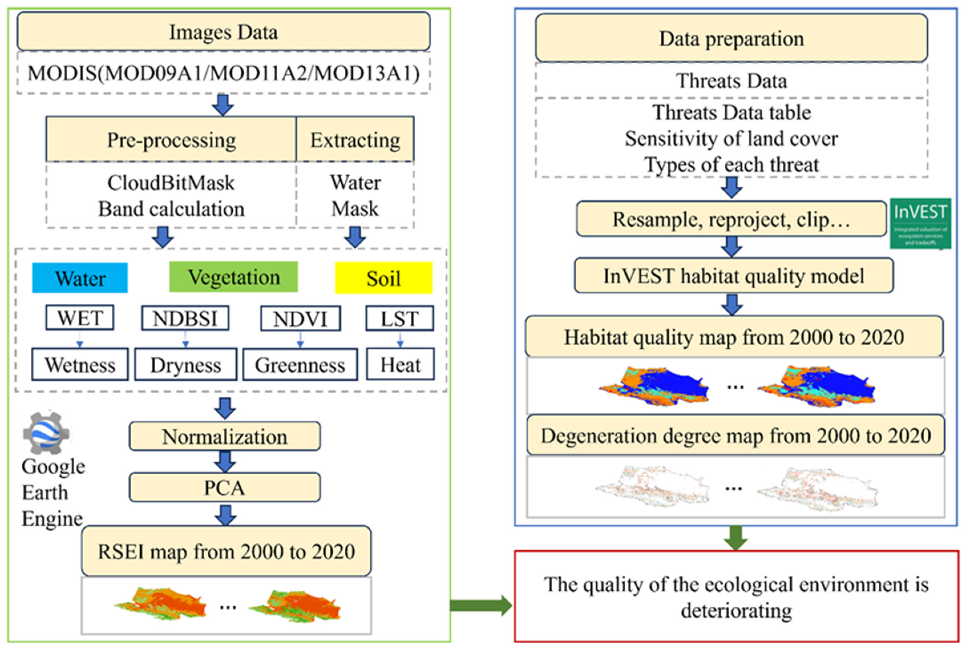
2.3.4. Construction of the RSEI

The Remote Sensing Ecological Index (RSEI) is a tool for assessing and analyzing the ecological quality of specific areas or ecosystems, leveraging remote sensing technology in conjunction with ecological indicators. Unlike traditional ecological observation techniques, RSEI offers comprehensive records of spatiotemporal data across the Earth’s surface, particularly at broader spatial scales. This allows for a rapid and convenient identification and monitoring of the ecological environment in any given area. The four critical components—green, wet, hot, and dry—are closely tied to human survival, making them frequent parameters for ecosystem evaluation in various studies [16]. The RSEI can be articulated as a function of these four indicators:

$$\mathrm{RSEI}=f\left(\mathrm{moisture},\mathrm{greenness},\mathrm{dryness},\mathrm{heat}\right)$$

(4)

Utilizing the indices WET, NDVI, NDBSI, and LST, which correspond to humidity, greenness, dryness, and heat, respectively, we derive the formula for the RSEI calculation:

$$\mathrm{RSEI}=f\left(\mathrm{WET},\mathrm{NDVI},\mathrm{NDBSI},\mathrm{LST}\right)$$

(5)

The primary growth period of vegetation, spanning from June to August, was selected for the calculation of the RSEI, which was computed annually from 2000 to 2020. Detailed calculation formulas for the RSEI and its components, along with data sources and PCA procedures, are provided in Appendix A.

2.3.5. Habitat Quality

The habitat quality (HQ) module of the InVEST model amalgamates land use and other factors that could potentially impact habitat quality such as building land, roads, and population density to generate a comprehensive habitat quality map [23]. This HQ model gauges habitat quality levels by evaluating the intensity of external pressures coupled with the sensitivity of ecosystems to these pressures. Generally, regions exhibiting high habitat quality demonstrate robust stability in their ecosystem structures and functions and tend to harbor higher biodiversity, and the converse is also true. We leveraged the habitat quality module of the InVEST model (version 3.7.0, Natural Capital Project, Stanford University, Stanford, CA, USA) to quantitatively assess habitat quality and evaluate the extent to which human activities influence the ecological system. The calculation formula is

$$Q_{xy}=H_j\left[1-\left({\displaystyle \frac{D_{xj}^Z}{D_{xj}^Z+K^Z}}\right)\right]$$

(6)

In the formula, Q_xy represents the habitat quality index of grid unit x in habitat type j, ranging from 0 to 1 (1 represents the best habitat quality); H_j is the habitat suitability degree of habitat type j; D_xj is the habitat degradation degree of grid unit x in habitat type j; z is the proportional coefficient, usually equal to 2.5; k is the half-saturation constant, usually taken as half of the maximum value of D_xj.

The detailed formulas and input data used in the habitat quality (HQ) model, including the calculation of stress factor impacts and sensitivity values for different land-use types, are provided in Appendix A.

2.3.6. Geographic Detector

The geographical detector is adept at identifying spatial heterogeneity in geographical entities, with the distinct advantage of detecting both numerical and qualitative data [35]. This study employs the R language GD package to leverage the factor detection capabilities of the geographical detector, thereby elucidating the impact of various factors on RSEI [36].

The calculation of the factorial detector typically involves the use of a q value, with the objective being to gauge the extent to which various factors explain the spatial difference of the dependent variable. This can be represented by the following formula:

$$q=1-\left({\displaystyle \sum }_{h=1}^L{N}_h{\delta }_h^2\right)/N{\delta }^2$$

(7)

In this context, L denotes the stratification (Strata) of variable Y or factor X, implying classification or division. N_h and N represent the count of units in layer h and the total region, respectively. The terms ${\delta }_h^2$ and ${\delta }^2$ refer to the variances of Y values within layer h and the entire region, respectively. q quantifies the degree of description of the RSEI provided by the exploratory factor, ranging from [0, 1]. A higher q value indicates a more potent explanatory capacity of the factor, signifying a greater contribution.

2.3.7. Hurst Index

The Hurst index is employed to quantitatively capture the persistence and anti-persistence characteristics of NDVI fluctuations [37]. When combined with the significant outcomes of the Mann–Kendall (MK) test (p < 0.05), it enhances the accuracy in forecasting future trends of time series data. Consider the NDVI time series denoted as NDVI (t), where t = 1, 2, 3, 4, …, n. For any positive integer τ, the subsequent formula can be derived:

$$NDV{I}_{\left(\tau \right)}={\displaystyle \frac{1}{\tau }}{\displaystyle \sum }_{i=1}^{\tau }NDV{I}_{\left(i\right)}$$

(8)

$$X_{\left(i,\tau \right)}={\displaystyle \sum }_{i=1}^i\left(NDV{I}_{\left(i\right)}-NDV{I}_{\left(\tau \right)}\right) 1\le i\le \tau$$

(9)

$$R_{\left(\tau \right)}=ma{x}_{1\epsilon t\epsilon \tau }X\left(t,\tau \right)-mi{n}_{1\epsilon t\epsilon \tau }X\left(t,\tau \right) \left(\tau =1,2,\cdots ,n\right)$$

(10)

$$S_{\left(\tau \right)}={\left[{\displaystyle \frac{1}{\tau }}{\displaystyle \sum }_{i=1}^{\tau }{\left(NDV{I}_{\left(i\right)}-NDV{I}_{\left(\tau \right)}\right)}^2\right]}^{1/2}$$

(11)

$${\displaystyle \frac{R_{\left(\tau \right)}}{S_{\left(\tau \right)}}}{\left(c\tau \right)}^H$$

(12)

$$\log {\left(R/S\right)}_n=a+H\times \log \left(n\right)$$

(13)

In the equation provided, NDVI_(τ) represents the differenced sequence, X(I, τ) is the average sequence, R(τ) denotes the range, and S(τ) signifies the standard deviation. The term H refers to the Hurst exponent, which has a value range of [0, 1]. A value of 0.5 is used as the classification criterion. When H is less than 0.5, it suggests that the time series data exhibit long-term autocorrelation, implying a potential trend reversal in the future. If H equals 0.5, it indicates that the trend of the time series data is random and lacks autocorrelation. Conversely, when H is greater than 0.5, it denotes that the time series data have long-term autocorrelation and are persistent, suggesting they may maintain their original trend. Overlay analysis with MK test results can further elucidate this: an “increase” suggests a potential shift to an increasing trend, while a “decrease” indicates a possible shift to a decreasing trend. A detailed classification and discussion of trend changes can be found in previous research [11].

Figure 2 presents the technical roadmap of this study.

3. Results

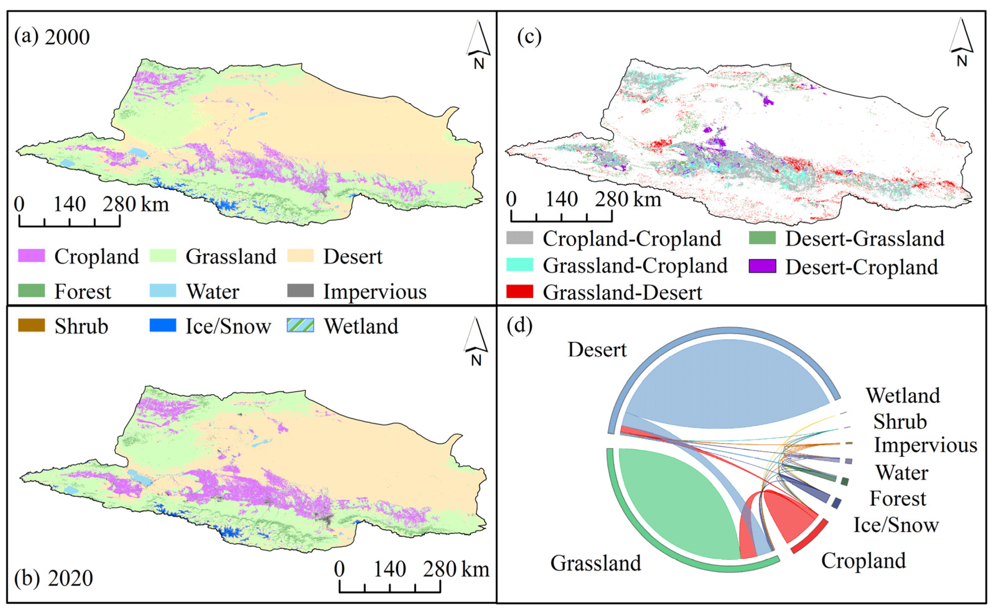
3.1. Land Use Change

The cropland in the study area is predominantly situated in the oasis region, with some plots on the middle and eastern slopes of the northern Tianshan Mountains bordering deserts (Figure 3a). Between 2000 and 2020, there was a steady expansion of the cropland area (Figure 3b,c). This growth primarily resulted from the reclamation of surrounding grasslands and deserts; 9.1% of the grasslands and 2.5% of the deserts were transformed into cropland (Figure 3d). Figure 3c illustrates the extensive reclamation of the oasis grasslands. In the interspersed desert–oasis regions adjacent to the Gurbantunggut Desert, there has been a degradation of grasslands, accounting for 8.1% of grasslands being converted into deserts. Conversely, 5.3% of deserts have been transformed into grasslands, predominantly in the western and northern sections of the study area. In total, the cropland area has expanded by 47.5%, grasslands have diminished by 8.9%, and deserts have contracted by 2.5%.

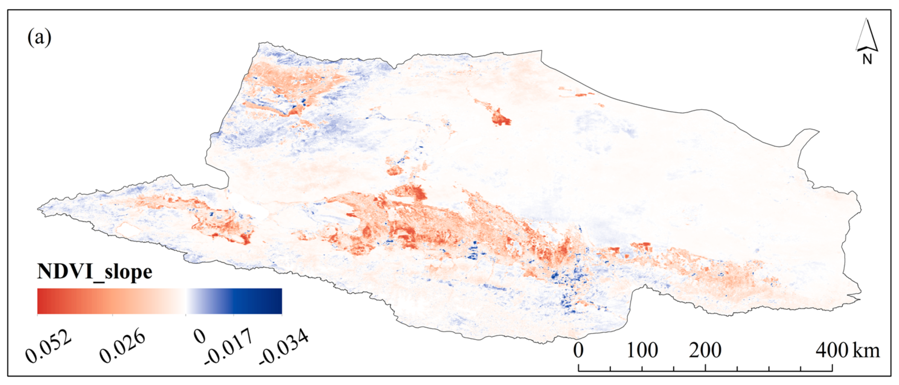
3.2. Temporal–Spatial Variations in NDVI

From 2000 to 2020, there was a significant increase in the regional Normalized Difference Vegetation Index (NDVI) (R² = 0.51, p < 0.01). After the removal of cropland, the NDVI continued to rise, but the change was not statistically significant (R² = 0.13, p > 0.05), suggesting minimal NDVI variation in areas other than cropland (Figure 4b). A significant positive correlation exists between the regional NDVI and the area of cropland, suggesting that the expansion of cultivation has contributed to the continuous increase in regional greenness (Figure 4c). The areas showing an increase in NDVI are primarily concentrated in oases, particularly in regions with intensive cultivation. Conversely, the NDVI decreased in the interspersed regions of oasis and desert. Additionally, vegetation degradation occurred in the high-altitude areas of the Emin River and Aibi Lake basins. The Gurbantunggut Desert, characterized by sparse vegetation coverage, exhibited non-significant changes in NDVI (Figure 4a).

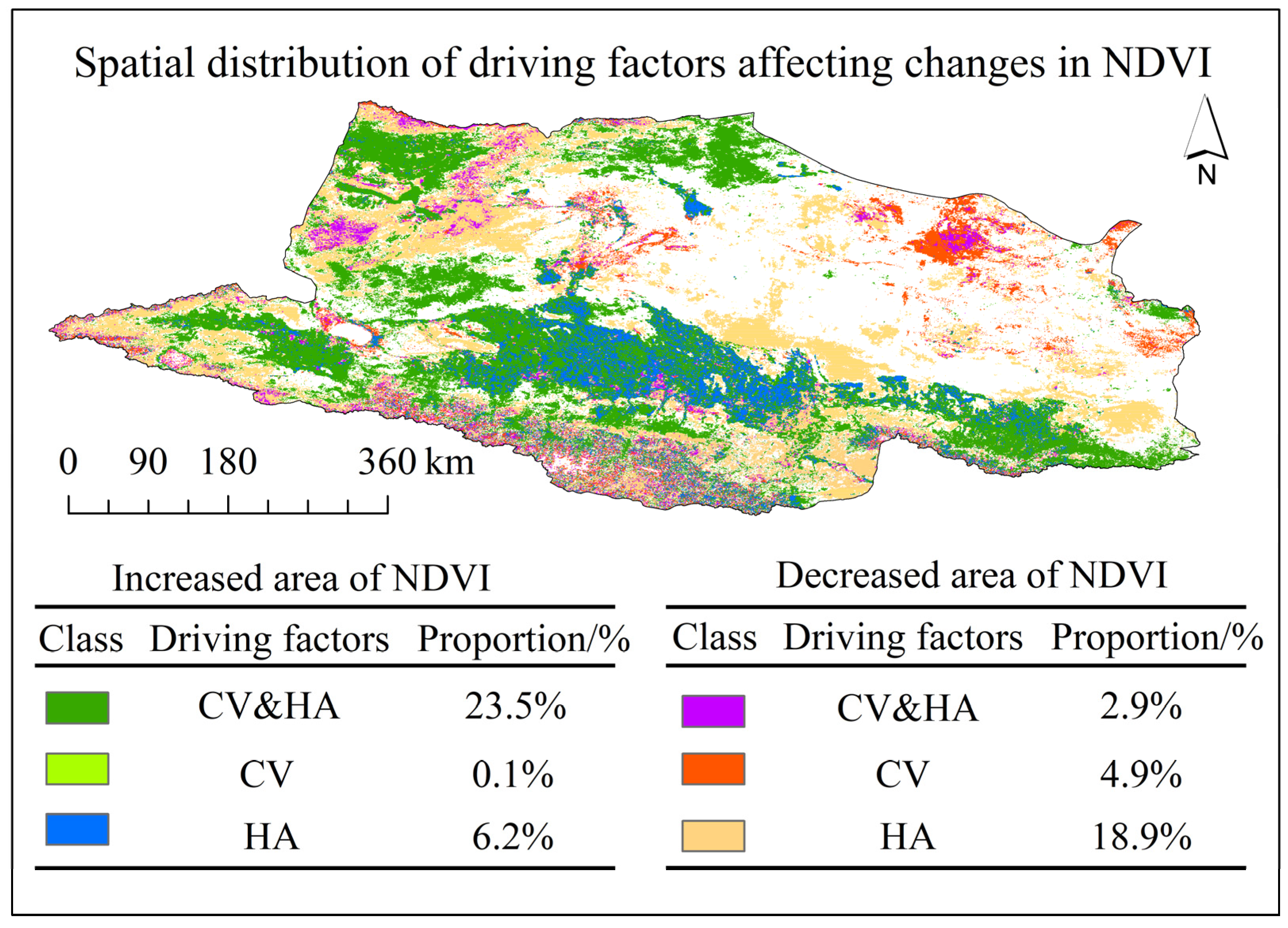
3.3. Analysis of Drivers of Change in NDVI

Figure 5 illustrates the spatial distribution of the driving forces behind NDVI changes. A notable 43.5% of the area showed no significant NDVI changes, primarily located in the Gurbantunggut Desert. This suggests that in these regions, the driving forces behind vegetation dynamics are either absent or minimal. Regions where NDVI increased due to a combination of climate change and human activities accounted for 23.5% of the area, while those solely influenced by human activities constituted 6.2%. These areas are mainly concentrated in oases with intensive cropland or newly reclaimed cropland, highlighting the significant role of human land use in driving vegetation change.

On the other hand, areas where vegetation change was driven by climate alone were negligible, accounting for just 0.1% of the total area. This reinforces the notion that, in this region, climate change has a marginal influence compared to human activities. In contrast, 26.7% of the total area showed a decrease in NDVI. Among these, 2.9% were influenced by both climate and human activities, and 4.9% were solely affected by climate factors. Notably, the most extensive vegetation degradation, affecting 18.9% of the total area, was primarily driven by human activities. These areas are most evident around the periphery of the oasis, with the alternating zones of oasis and desert showing pronounced degradation patterns. Additionally, certain grasslands in mountainous regions exhibit degradation resulting from overgrazing and other anthropogenic pressures.

In conclusion, while climate change has a limited influence on vegetation coverage in the study area, the impact of human activities, particularly through land use changes and overgrazing, is far more significant. This underscores the need for focused land management strategies to mitigate further vegetation degradation in these vulnerable regions.

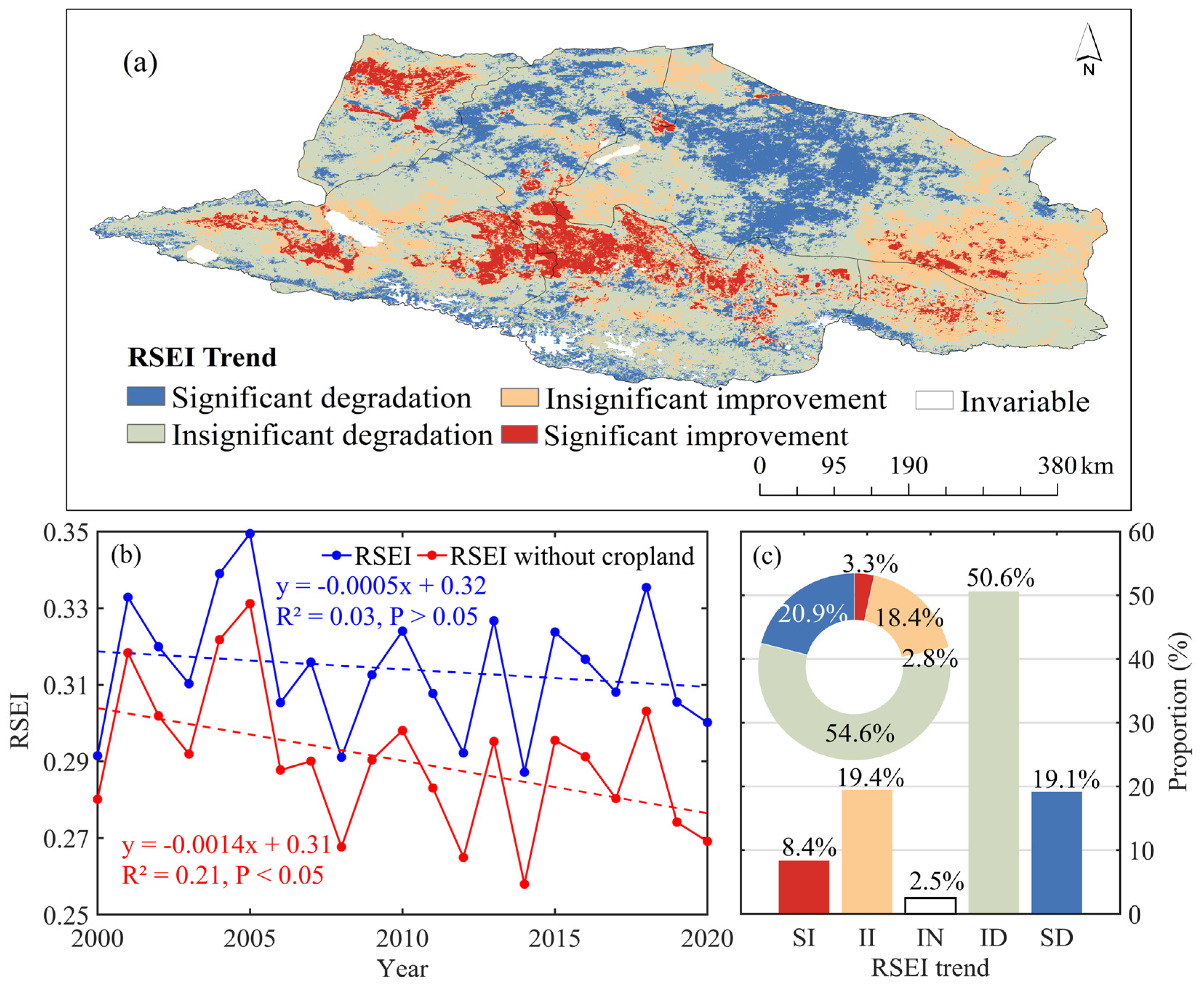
3.4. Temporal–Spatial Variations in RSEI

From Figure 6b, it is evident that the region’s overall ecological environment quality exhibits a non-significant decline (p = 0.464). The average RSEI peaked in 2005 at 0.35 and plummeted to its lowest in 2014 at 0.29. Notably, upon excluding cropland from the calculations, there was a significant decrease in the average RSEI (p < 0.05), ranging from 0.33 in 2005 to 0.26 in 2014. Employing methods like the Theil–Sen and Mann–Kendall trend tests, we delved into the spatial variation trends of RSEI between 2000 and 2020 within this region. To ensure a comprehensive assessment, both the entire region and an area excluded from cropland were evaluated. As depicted in Figure 6a, when cropland is factored out, there is a discernible degradation in the regional ecological environment’s quality. This decline is particularly pronounced in the interspersed oasis and desert zones, as well as in most parts of the Gurbantunggut Desert. Additionally, forest and grassland areas in mountainous regions also display a downward trajectory. According to Figure 6c, the distributions for areas showing significant improvement, slight improvement, no change, slight deterioration, and significant deterioration are 8.3%, 12.4%, 9.5%, 50.60%, and 19.2%, respectively. However, after excluding cropland, these percentages are recalculated to be 3.3%, 18.4%, 2.8%, 54.6%, and 20.9%, respectively.

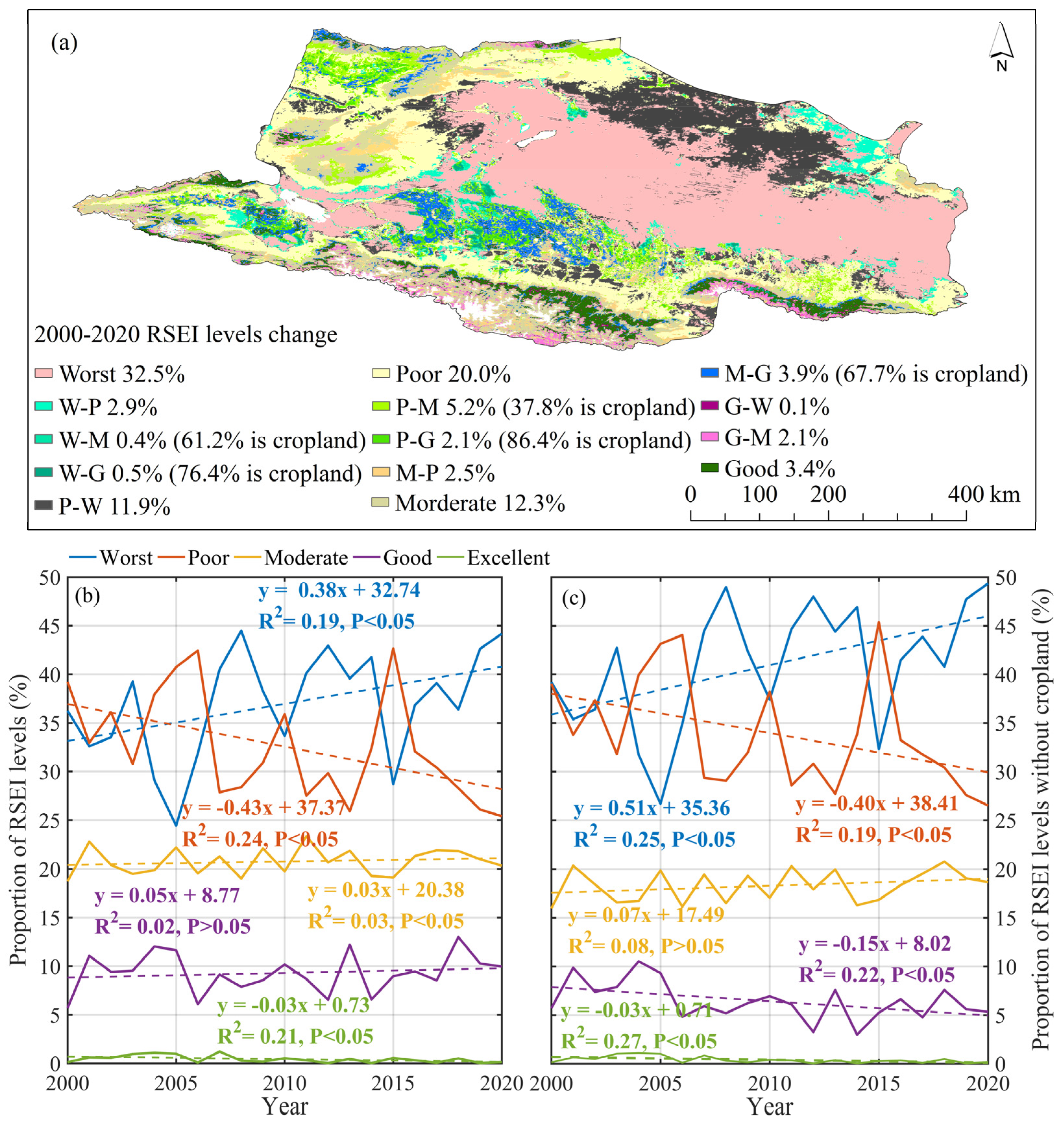
3.5. Spatiotemporal Analysis of RSEI Levels

This study employs the natural breakpoint method to categorize RSEI into five levels, each with an interval of 0.2. Under this classification, RSEI is deemed “poor” within the range of 0 to 0.2, “relatively poor” from 0.2 to 0.4, “moderate” between 0.4 and 0.6, “good” from 0.6 to 0.8, and “excellent” from 0.8 to 1. The study further examines the trends in the proportion of these RSEI levels from 2000 to 2020, taking into account both the overall region and cropland removal. Figure 7b,c illustrate that the predominant ecological quality levels in the region are poor and relatively poor, with their combined proportion reaching 75.46% in 2000. It is also evident that the proportion of the worst ecological quality in the region has significantly increased (R² = 0.19, p < 0.05), a trend that becomes more pronounced after cropland removal (R² = 0.24, p < 0.05). Conversely, the proportion of poor ecological quality has notably declined (R² = 0.24, p < 0.05), suggesting a continuous deterioration of areas with poor ecological quality. The regions with moderate ecological quality have remained relatively stable in both scenarios (p > 0.05), while those with excellent ecological quality are minimal and have seen a significant decrease in both cases (p < 0.05). The proportion of good ecological quality has remained relatively stable across the entire region (R² = 0.02, p > 0.05), but it has significantly decreased post-cropland removal (R² = 0.22, p < 0.05). The expansion of cropland has contributed to an overall increase in regional greenness, obscuring the reality of ecological degradation to some extent. However, the trend towards ecological environment deterioration becomes more evident once cropland is removed.

Figure 7a illustrates the spatial variation of the RSEI ecological quality grade in the study area from 2000 to 2020. The area that remained stable between 2000 and 2020 constituted 68.2% of the region, while the areas where the ecological quality remained the worst represented 32.5% of the total area, predominantly the Gurbantunggut Desert. The area where the ecological quality remained good constituted a mere 3.4% of the region, primarily the forests on the Tianshan Mountains. The area that deteriorated from poor to the worst accounted for 11.9% of the region, primarily located in the north of Gurbantunggut and along the edge of the oasis, which bordered the desert and grassland. The areas that improved from poor to moderate and good represented 5.2% and 2.1% of the region, respectively, mainly situated in the middle of the northern slope of the Tianshan Mountains. It is evident that these improvements were primarily due to these areas being reclamated as cropland, accounting for 76.4% and 86.4% in W-G and P-G, respectively. There was also a certain degree of vegetation degradation in the mountains, with G-M accounting for 2.1%, mainly in high-altitude areas. However, the trend of degradation continues to dominate the overall ecological environment quality of the region.

3.6. Detecting the Driving Factors for RSEI Spatial Differentiation

The single-factor detection results reveal that the q values for the selected influencing factors in this study are all below 0.01. This suggests that the independent variables exert a significant influence on the spatial heterogeneity of the RSEI.

Table 2. q value of each influencing factors.

Influence Factor	2000 q Value	2005 q Value	2010 q Value	2015 q Value	2020 q Value	2000–2020 q Value
NDVI	0.61	0.7	0.7	0.75	0.78	0.72
WET	0.18	0.43	0.43	0.47	0.53	0.58
LST	0.79	0.69	0.69	0.62	0.57	0.48
NDBSI	0.47	0.51	0.51	0.63	0.65	0.21
LAI	0.53	0.63	0.63	0.71	0.74	0.54
Elev	0.55	0.41	0.41	0.23	0.26	-
Prec	0.29	0.24	0.24	0.1	0.18	0.04
Temp	0.49	0.32	0.32	0.16	0.23	0.07
LUCC	0.34	0.4	0.4	0.46	0.48	0.41

presents the single-factor detection results spanning from 2000 to 2020. While the primary driving factors of the RSEI (remote sensing index of ecological environment) in the study area have undergone some variations between 2000 and 2020, vegetation-related factors such as NDVI and LAI consistently maintain a dominant role. Additionally, the q values for LST and NDBSI are notably elevated. The effects of WET and LUCC on the RSEI remain relatively stable, whereas the impacts of other factors appear to be somewhat diminished. Upon evaluating the sensitivity slope values of these influencing factors in relation to RSEI changes from 2000 to 2020, we further explored their implications on the quality alterations of the ecological environment. The findings can be ranked as follows: NDVI > WET > LAI > LUCC > NDBSI > HFP > Temp > Prec. To encapsulate, throughout the entire research duration, vegetation changes have consistently played a predominant role in determining the ecological quality of the study area. Simultaneously, alterations in land use types have also significantly influenced ecological environment changes across the region, while the effects of meteorological factor changes have been identified as relatively minor.

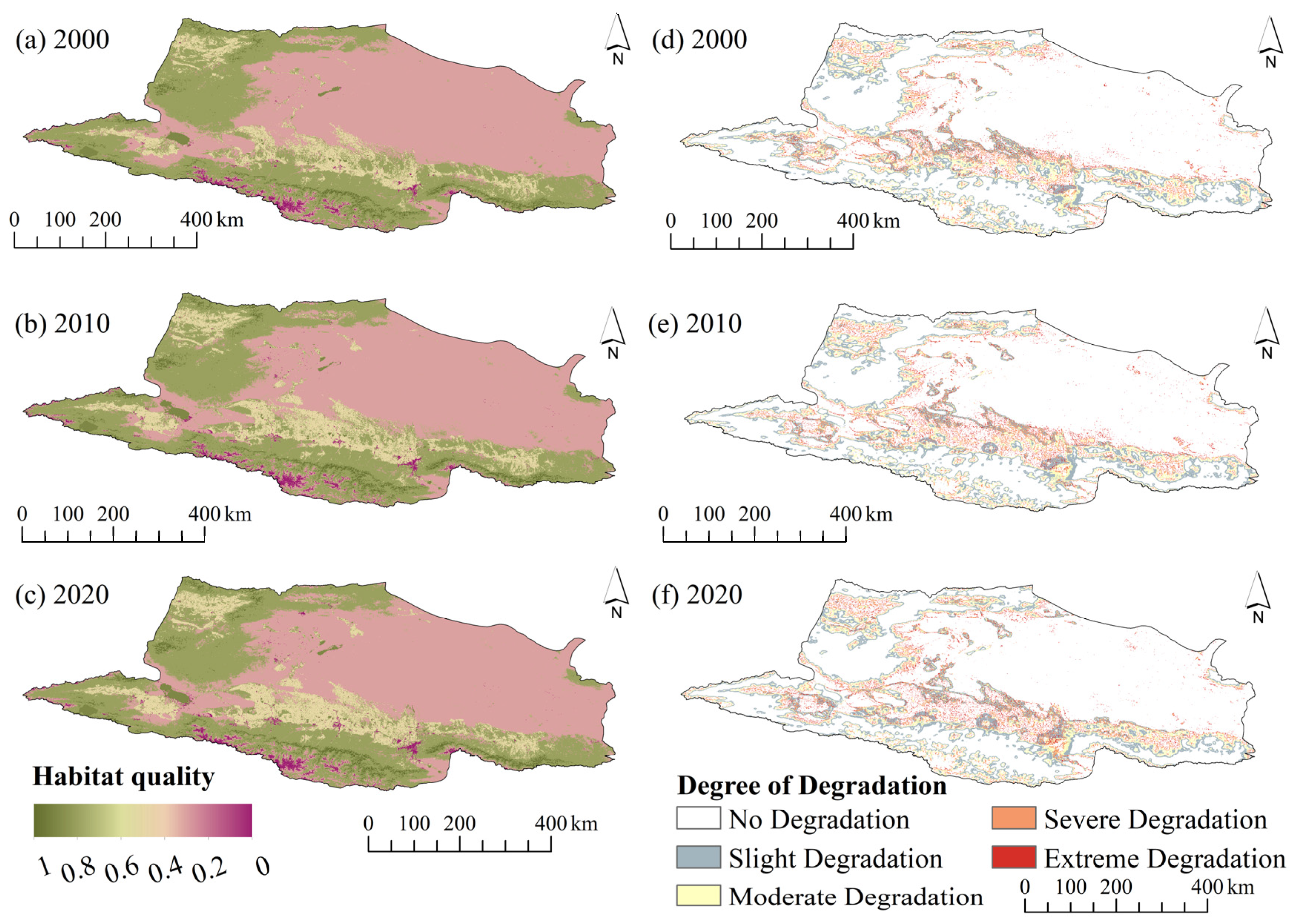
3.7. Habitat Quality and Degradation Variations in Space and Time

The spatial distribution analysis reveals a progressive expansion of low-quality habitat areas, with regions of intensive cropland concentration showing the most significant declines in habitat quality (Figure 8). Areas undergoing substantial degradation are primarily located within oases, largely as a result of cropland expansion replacing grasslands and other natural vegetation. Moreover, vegetation in high-altitude regions and along the margins of oases continues to deteriorate (Figure 8), further highlighting the compounding ecological challenges in these areas.

Figure 9 demonstrates a statistically significant decline in habitat quality between 2000 and 2020 (p < 0.05), accompanied by a highly significant increase in the degree of degradation (p < 0.01). These trends are particularly pronounced within a 2 km radius of cropland peripheries. It is noteworthy that prior to 2008, habitat quality exhibited a period of improvement, likely driven by afforestation and other ecological restoration initiatives. However, after 2008, habitat quality declined markedly, coinciding with the widespread implementation of water-saving irrigation technologies across the study area. This transition was followed by substantial cropland expansion.

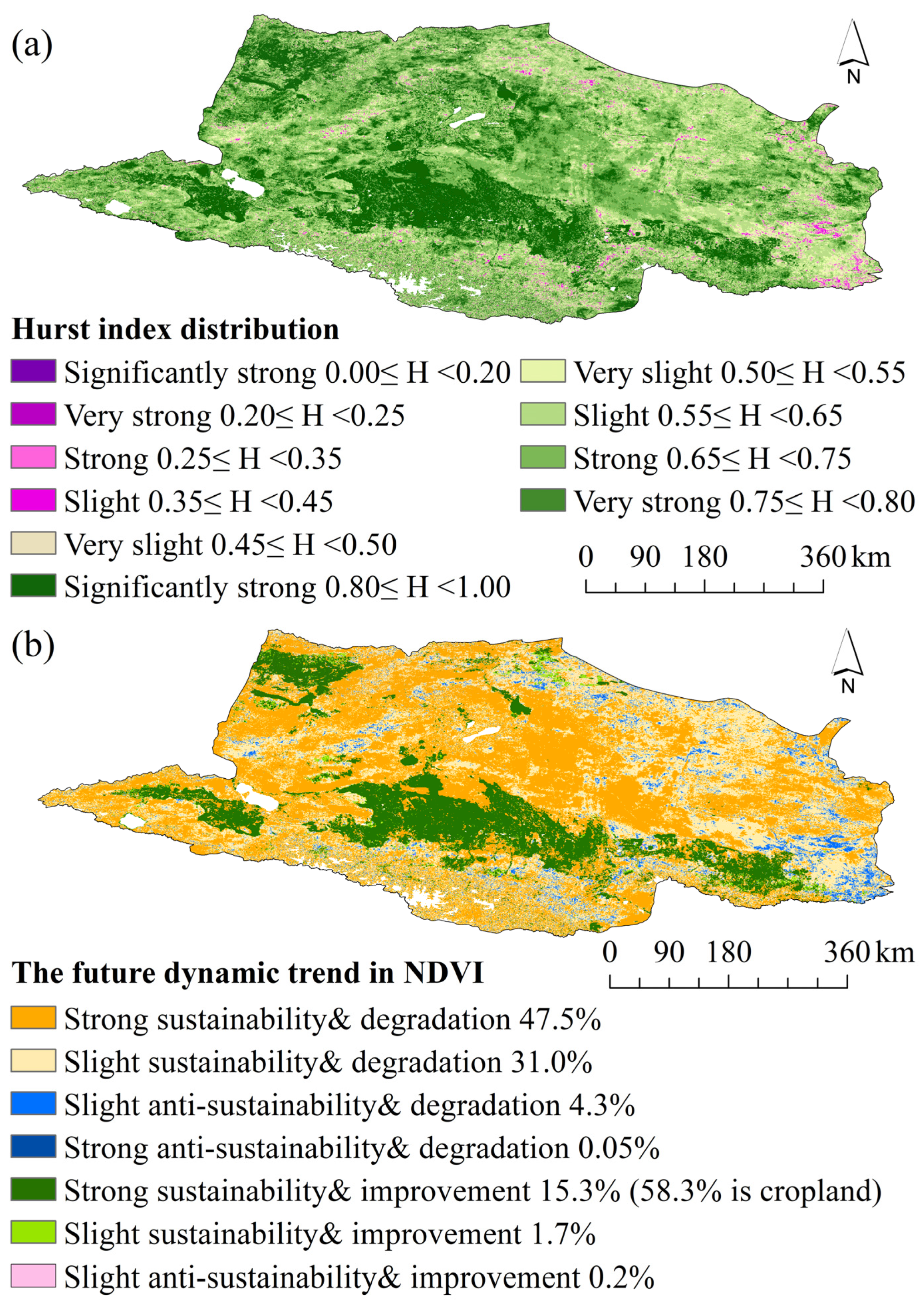
3.8. Future Trends Change in NDVI

Our analysis revealed that regional ecological environment quality was closely associated with changes in NDVI, which served as a key indicator reflecting the impacts of underlying drivers such as land use change and human activities. Consequently, we employed the Hurst index to characterize vegetation sustainability and forecast future vegetation trajectories. Figure 10a presents the spatial distribution of sustainability as per the Hurst index. The average Hurst index value for the region between 2000 and 2020 stood at 0.69. Notably, areas with a Hurst index exceeding 0.5 constituted 95.4% of the region, with 62.7% of these areas displaying an index above 0.65, indicating strong sustainability. These trends suggest that the vegetation in these regions will likely follow historical patterns. Areas with a Hurst index below 0.5 are minimal and are primarily located in the Gurbantunggut Desert and on the outskirts of oases.

Figure 10b illustrates the predictive outcomes of future dynamic trends in NDVI, categorized based on sustainability and degradation degree. The analytical results reveal that the regions with pronounced sustainability and degradation represent the most substantial proportion, constituting 47.5%, succeeded by areas exhibiting slight sustainability and degradation, which comprise 31.0%. This suggests that vegetation within these regions will likely experience continued degradation, attributable to both climatic changes and human interventions. Conversely, zones demonstrating robust sustainability and enhancement constitute merely 15.3% of the study area, with 58.3% of the region being cropland. Thus, after accounting for cultivated areas, only 6.4% remains for potential continuous vegetation improvement. Predominantly, the dynamic trend of vegetation within the study area is characterized by degradation, with areas showing improvement being markedly limited. This underscores the ongoing challenges faced by the sustainable development of regional ecosystems.

4. Discussion

4.1. Cropland Expansion and the ‘Greening’ Phenomenon

The expansion of cropland has been a major driver of increased vegetation coverage, resulting in a noticeable “greening” trend. Although China accounts for only 6.6% of the global vegetation area, it contributes 25% of the worldwide net increase in leaf area, with croplands accounting for 32% of this growth [38]. Our study shows that cropland in the research area has expanded by 48%, equating to an annual growth rate of 52.49 thousand hectares. This has been accompanied by a significant increase in the regional NDVI, at a rate of 0.003 year⁻¹. However, when cropland is excluded from the analysis, the NDVI growth rate drops to 0.001 year⁻¹. Spatially, areas with higher NDVI values are predominantly found in oases, which suggests that the observed NDVI increase is largely attributed to cropland expansion rather than a genuine restoration of natural vegetation. Furthermore, as this study did not fully control for the influence of ecological restoration initiatives such as afforestation, the true growth rate of NDVI in natural vegetation may be considerably lower or even exhibit a downward trend.

The conversion of natural ecosystems to cropland in arid regions has led to the degradation of native vegetation. Our analysis reveals that 9.1% of grasslands and 2.5% of deserts in the study area have been converted into cropland [8]. This transformation has resulted in an apparent improvement in the RSEI, with 76.4% of the area shifting from poor to good and 86.4% from relatively poor to good due to cultivation. These changes suggest that the presence of cropland artificially elevates the average NDVI and RSEI values for the region, often misinterpreted as ecological improvements. This “greening” phenomenon, however, masks the underlying ecological alterations, particularly in arid oases and desert ecosystems, where the replacement of natural habitats with agricultural land significantly reduces biodiversity and ecosystem functions.

4.2. The Risks Behind “Greening“

The “greening” effect associated with cropland expansion often masks the underlying ecological risks, which threaten both ecosystem stability and regional sustainable development. Our research reveals a significant decline in habitat quality in the study area, with degradation levels sharply increasing. The expansion of cropland has disrupted the equilibrium of natural ecosystems, particularly impacting the stability of grassland and desert ecosystems [8]. Although these ecosystems exhibit lower vegetation coverage, they provide essential ecological functions, including soil and water conservation, carbon storage, and biodiversity protection [39,40]. However, the spread of cropland has replaced native vegetation with crops, occupying natural habitats and drastically reducing species diversity. This shift, particularly the replacement of drought- and salt-tolerant local plants with intensive agricultural production, has undermined the resilience of local biodiversity and ecosystems. Consequently, some sensitive species are at risk of extinction [41,42].

The expansion of cropland has exacerbated the water resource crisis. Studies indicate that cropland expansion in northwest China has significantly increased agricultural water consumption, depleting terrestrial water reserves [43]. This pressure is driven not only by the expansion of irrigated areas but also by changes in cropping patterns, such as the shift to water-intensive crops like cotton following the adoption of water-saving technologies. These changes have further heightened the demand for agricultural water [26,27]. Excessive agricultural water use has led to groundwater depletion and contributed to soil salinization [44,45]. Moreover, the prioritization of water resources for irrigation reduces the water available for other ecosystems, accelerating the degradation of natural vegetation [27,46]. Our findings suggest that human activities contribute to 18.9% of the vegetation degradation in the region, primarily around cropland edges, especially in the oasis–desert interface. This is likely due to reduced groundwater levels and diminished lateral recharge following the adoption of water-saving irrigation techniques [27,46]. Research indicates that shrubs in the Gurbantunggut Desert, such as Haloxylon ammodendron, depend largely on groundwater [47,48]. A reduction in vegetation cover accelerates desertification, and the degradation of such vegetation and ecosystem functions is often irreversible, with recovery potentially taking decades or more [2,41].

4.3. Future Vegetation Changes

The geographic detector results indicate that greenness is the primary determinant of the regional RSEI, with vegetation growth playing a crucial role in maintaining the ecological integrity of the region. This study forecasts future trends in regional NDVI by analyzing historical data from 2000 to 2020 using the Hurst index. The findings show that 47.5% of the region is experiencing significant and persistent degradation, 15.3% is undergoing robust and sustained improvement, while 58.3% of the area is covered by cropland.

Based on a review of existing research and land-use trends, future vegetation changes in the study area may be dynamic and unpredictable. Factors such as optimized irrigation systems, ecological restoration projects, and the introduction of artificial vegetation could enhance vegetation coverage in the oasis. However, the cumulative impact of cropland expansion and overexploitation of water resources presents a significant long-term threat to the region’s ecological environment. Particularly in the context of climate change, the frequency and intensity of extreme climate events, such as droughts and sandstorms, are likely to increase, further exacerbating the risk of vegetation degradation [49].

Vegetation restoration in desert and mountainous regions is constrained by harsh natural conditions and ecosystem vulnerability. Such efforts require extensive, costly ecological engineering over the long term [6]. Current ecological protection policies and resource allocation are predominantly focused on oasis areas, neglecting the ecological challenges in desert and mountainous regions. If the conflict between agricultural and ecological water consumption is not addressed effectively, the expansion of vegetation in oasis areas may lead to further degradation of desert and mountainous ecosystems. This imbalanced development model threatens the health of natural ecosystems and undermines the ecological services and sustainable development potential of the entire region.

5. Conclusions

This study demonstrates that the increasing trend of NDVI in Northwest China’s mountain–oasis–desert ecosystem from 2000 to 2020 does not represent genuine ecological improvement. Instead, the apparent “greening” is largely driven by cropland expansion, with significant NDVI and RSEI increases concentrated in oasis areas. When croplands are excluded, ecological quality—as measured by RSEI—declines substantially, with 20.9% of the region exhibiting ecological degradation. The InVEST habitat quality model further confirms this trend, showing widespread habitat quality loss and a 9.1% conversion of grasslands into croplands. Long-term vegetation dynamics assessed through the Hurst index reveal that nearly half (47.5%) of the region’s vegetation is projected to continue degrading. These findings indicate that agricultural expansion is masking environmental degradation in fragile dryland ecosystems. Therefore, it is imperative to strategically manage land use in arid regions, balancing short-term agricultural development with long-term ecological sustainability.

References

1. Lian, X.; Piao, S.; Chen, A.; Huntingford, C.; Fu, B.; Li, L.Z.X.; Huang, J.; Sheffield, J.; Berg, A.M.; Keenan, T.F.; et al. Multifaceted characteristics of dryland aridity changes in a warming world. Nat. Rev. Earth Environ. 2021, 2, 232–250. [Google Scholar] [CrossRef]
2. Berdugo, M.; Kéfi, S.; Soliveres, S.; Maestre, F.T. Plant spatial patterns identify alternative ecosystem multifunctionality states in global drylands. Nat. Ecol. Evol. 2017, 1, 0003. [Google Scholar] [CrossRef] [PubMed]
3. Niu, G.; Zheng, Y.; Han, F.; Qin, H. The nexus of water, ecosystems and agriculture in arid areas: A multiobjective optimization study on system efficiencies. Agric. Water Manag. 2019, 223, 105697. [Google Scholar] [CrossRef]
4. Xu, W.; Su, X. Challenges and impacts of climate change and human activities on groundwater-dependent ecosystems in arid areas—A case study of the Nalenggele alluvial fan in NW China. J. Hydrol. 2019, 573, 376–385. [Google Scholar] [CrossRef]
5. Ge, G.; Shi, Z.; Zhu, Y.; Yang, X.; Hao, Y. Land use/cover classification in an arid desert-oasis mosaic landscape of China using remote sensed imagery: Performance assessment of four machine learning algorithms. Glob. Ecol. Conserv. 2020, 22, e00971. [Google Scholar] [CrossRef]
6. Li, C.J.; Fu, B.J.; Wang, S.; Stringer, L.C.; Wang, Y.P.; Li, Z.D.; Liu, Y.X.; Zhou, W.X. Drivers and impacts of changes in China’s drylands. Nat. Rev. Earth Environ. 2021, 2, 858–873. [Google Scholar] [CrossRef]
7. Xue, J.; Gui, D.; Lei, J.; Sun, H.; Zeng, F.; Mao, D.; Jin, Q.; Liu, Y. Oasification: An unable evasive process in fighting against desertification for the sustainable development of arid and semiarid regions of China. Catena 2019, 179, 197–209. [Google Scholar] [CrossRef]
8. Chen, P.; Wang, S.; Liu, Y.X.; Wang, Y.J.; Song, J.X.; Tang, Q.; Yao, Y.; Wang, Y.P.; Wu, X.T.; Wei, F.L.; et al. Spatio-Temporal Dynamics of Aboveground Biomass in China’s Oasis Grasslands Between 1989 and 2021. Earth’s Future 2024, 12, e2023EF003944. [Google Scholar] [CrossRef]
9. Tietjen, B.; Schlaepfer, D.R.; Bradford, J.B.; Lauenroth, W.K.; Hall, S.A.; Duniway, M.C.; Hochstrasser, T.; Jia, G.; Munson, S.M.; Pyke, D.A.; et al. Climate change-induced vegetation shifts lead to more ecological droughts despite projected rainfall increases in many global temperate drylands. Glob. Chang. Biol. 2017, 23, 2743–2754. [Google Scholar] [CrossRef]
10. Wang, Y.; Li, Y. Land exploitation resulting in soil salinization in a desert-oasis ecotone. Catena 2013, 100, 50–56. [Google Scholar] [CrossRef]
11. He, L.; Guo, J.; Jiang, Q.; Zhang, Z.; Yu, S. How did the Chinese Loess Plateau turn green from 2001 to 2020? An explanation using satellite data. Catena 2022, 214, 106246. [Google Scholar] [CrossRef]
12. Li, X.; Wang, K.; Huntingford, C.; Zhu, Z.; Peñuelas, J.; Myneni, R.B.; Piao, S. Vegetation greenness in 2023. Nat. Rev. Earth Environ. 2024, 5, 241–243. [Google Scholar] [CrossRef]
13. Zhang, J.; Zhang, P.; Deng, X.; Ren, C.; Deng, M.; Wang, S.; Lai, X.; Long, A. Study on the Spatial and Temporal Trends of Ecological Environment Quality and Influencing Factors in Xinjiang Oasis. Remote Sens. 2024, 16, 1980. [Google Scholar] [CrossRef]
14. Gorelick, N.; Hancher, M.; Dixon, M.; Ilyushchenko, S.; Thau, D.; Moore, R. Google Earth Engine: Planetary-scale geospatial analysis for everyone. Remote Sens. Environ. 2017, 202, 18–27. [Google Scholar] [CrossRef]
15. Weng, Q.H.; Lu, D.S.; Schubring, J. Estimation of land surface temperature-vegetation abundance relationship for urban heat island studies. Remote Sens. Environ. 2004, 89, 467–483. [Google Scholar] [CrossRef]
16. Xu, H.; Wang, Y.; Guan, H.; Shi, T.; Hu, X. Detecting Ecological Changes with a Remote Sensing Based Ecological Index (RSEI) Produced Time Series and Change Vector Analysis. Remote Sens. 2019, 11, 2345. [Google Scholar] [CrossRef]
17. Aizizi, Y.; Kasimu, A.; Liang, H.; Zhang, X.; Wei, B.; Zhao, Y.; Ainiwaer, M. Evaluation of Ecological Quality Status and Changing Trend in Arid Land Based on the Remote Sensing Ecological Index: A Case Study in Xinjiang, China. Forests 2023, 14, 1830. [Google Scholar] [CrossRef]
18. Tang, J.; Zhou, L.; Dang, X.; Hu, F.; Yuan, B.; Yuan, Z.; Wei, L. Impacts and predictions of urban expansion on habitat quality in the densely populated areas: A case study of the Yellow River Basin, China. Ecol. Indic. 2023, 151, 110320. [Google Scholar] [CrossRef]
19. Yang, H.; Yu, J.; Xu, W.; Wu, Y.; Lei, X.; Ye, J.; Geng, J.; Ding, Z. Long-time series ecological environment quality monitoring and cause analysis in the Dianchi Lake Basin, China. Ecol. Indic. 2023, 148, 110084. [Google Scholar] [CrossRef]
20. Zhang, W.; Liu, Z.; Qin, K.; Dai, S.; Lu, H.; Lu, M.; Ji, J.; Yang, Z.; Chen, C.; Jia, P. Long-Term Dynamic Monitoring and Driving Force Analysis of Eco-Environmental Quality in China. Remote Sens. 2024, 16, 1028. [Google Scholar] [CrossRef]
21. Aizizi, Y.; Kasimu, A.; Liang, H.; Zhang, X.; Zhao, Y.; Wei, B. Evaluation of ecological space and ecological quality changes in urban agglomeration on the northern slope of the Tianshan Mountains. Ecol. Indic. 2023, 146, 109896. [Google Scholar] [CrossRef]
22. Yohannes, H.; Soromessa, T.; Argaw, M.; Dewan, A. Spatio-temporal changes in habitat quality and linkage with landscape characteristics in the Beressa watershed, Blue Nile basin of Ethiopian highlands. J. Environ. Manag. 2020, 281, 111885. [Google Scholar] [CrossRef]
23. Aneseyee, A.B.; Noszczyk, T.; Soromessa, T.; Elias, E. The InVEST Habitat Quality Model Associated with Land Use/Cover Changes: A Qualitative Case Study of the Winike Watershed in the Omo-Gibe Basin, Southwest Ethiopia. Remote Sens. 2020, 12, 1103. [Google Scholar] [CrossRef]
24. Wu, C.; Deng, L.; Huang, C.; Chen, Y.; Peng, C. Effects of vegetation restoration on soil nutrients, plant diversity, and its spatiotemporal heterogeneity in adesert-oasisecotone. Land Degrad. Dev. 2021, 32, 670–683. [Google Scholar] [CrossRef]
25. Li, Y.; Wang, Y.G.; Houghton, R.A.; Tang, L. Hidden carbon sink beneath desert. Geophys. Res. Lett. 2015, 42, 5880–5887. [Google Scholar] [CrossRef]
26. Wang, Y.; Long, A.; Xiang, L.; Deng, X.; Pei, Z.; Yang, H.; Jie, W.; Yang, L. The verification of Jevons’ paradox of agricultural Water conservation in Tianshan District of China based on Water footprint. Agric. Water Manag. 2020, 239, 106163. [Google Scholar] [CrossRef]
27. Zhao, N.; Zheng, X.; Zhang, B.; Tian, S.; Du, L.; Li, Y. Does water-saving irrigation truly conserve water? Yes and No. Agric. Water Manag. 2025, 311, 109399. [Google Scholar] [CrossRef]
28. Peng, S.; Ding, Y.; Liu, W.; Li, Z. 1 km monthly temperature and precipitation dataset for China from 1901 to 2017. Earth Syst. Sci. Data 2019, 11, 1931–1946. [Google Scholar] [CrossRef]
29. Peng, S.; Ding, Y.; Wen, Z.; Chen, Y.; Cao, Y.; Ren, J. Spatiotemporal change and trend analysis of potential evapotranspiration over the Loess Plateau of China during 2011–2100. Agric. For. Meteorol. 2017, 233, 183–194. [Google Scholar] [CrossRef]
30. Peng, S.; Gang, C.; Cao, Y.; Chen, Y. Assessment of climate change trends over the Loess Plateau in China from 1901 to 2100. Int. J. Climatol. 2018, 38, 2250–2264. [Google Scholar] [CrossRef]
31. Ding, Y.; Peng, S. Spatiotemporal trends and attribution of drought across China from 1901–2100. Sustainability 2020, 12, 477. [Google Scholar] [CrossRef]
32. Yang, J.; Huang, X. The 30 m annual land cover dataset and its dynamics in China from 1990 to 2019. Earth Syst. Sci. Data 2021, 13, 3907–3925. [Google Scholar] [CrossRef]
33. Aguiar, R.; Collares-Pereira, M.; Conde, J. Simple procedure for generating sequences of daily radiation values using a library of Markov transition matrices. Sol. Energy 1988, 40, 269–279. [Google Scholar] [CrossRef]
34. Evans, J.; Geerken, R. Discrimination between climate and human-induced dryland degradation. J. Arid Environ. 2004, 57, 535–554. [Google Scholar] [CrossRef]
35. Wang, J.; Xu, C. Geodetector: Principle and prospective. Acta Geogr. Sin. 2017, 72, 116–134. [Google Scholar] [CrossRef]
36. Song, Y.; Wang, J.; Ge, Y.; Xu, C. An optimal parameters-based geographical detector model enhances geographic characteristics of explanatory variables for spatial heterogeneity analysis: Cases with different types of spatial data. GISci. Remote Sens. 2020, 57, 593–610. [Google Scholar] [CrossRef]
37. Jiang, W.; Yuan, L.; Wang, W.; Cao, R.; Zhang, Y.; Shen, W.M. Spatio-temporal analysis of vegetation variation in the Yellow River Basin. Ecol. Indic. 2015, 51, 117–126. [Google Scholar] [CrossRef]
38. Chen, C.; Park, T.; Wang, X.; Piao, S.; Xu, B.; Chaturvedi, R.K.; Fuchs, R.; Brovkin, V.; Ciais, P.; Fensholt, R.; et al. China and India lead in greening of the world through land-use management. Nat. Sustain. 2019, 2, 122–129. [Google Scholar] [CrossRef]
39. Thomas, F.M.; Foetzki, A.; Arndt, S.K.; Bruelheide, H.; Gries, D.; Li, X.; Zeng, F.; Zhang, X.; Runge, M. Water use by perennial plants in the transition zone between river oasis and desert in NW China. Basic Appl. Ecol. 2006, 7, 253–267. [Google Scholar] [CrossRef]
40. Wang, G.; Munson, S.M.; Yu, K.; Chen, N.; Gou, Q. Ecological effects of establishing a 40-year oasis protection system in a northwestern China desert. Catena 2020, 187, 104374. [Google Scholar] [CrossRef]
41. Sawut, M.; Eziz, M.; Tiyip, T. The effects of land-use change on ecosystem service value of desert oasis: A case study in Ugan-Kuqa River Delta Oasis, China. Can. J. Soil Sci. 2013, 93, 99–108. [Google Scholar] [CrossRef]
42. Su, Y.Z.; Zhao, W.Z.; Su, P.X.; Zhang, Z.H.; Wang, T.; Ram, R. Ecological effects of desertification control and desertified land reclamation in an oasis-desert ecotone in an and region: A case study in Hexi Corridor, northwest China. Ecol. Eng. 2007, 29, 117–124. [Google Scholar] [CrossRef]
43. Lai, J.M.; Li, Y.A.; Chen, J.L.; Niu, G.Y.; Lin, P.R.; Li, Q.; Wang, L.X.; Han, J.M.; Luo, Z.Q.; Sun, Y. Massive crop expansion threatens agriculture and water sustainability in northwestern China. Environ. Res. Lett. 2022, 17, 034003. [Google Scholar] [CrossRef]
44. Abliz, A.; Tiyip, T.; Ghulam, A.; Halik, Ü.; Ding, J.L.; Sawut, M.; Zhang, F.; Nurmemet, I. Effects of shallow groundwater table and salinity on soil salt dynamics in the Keriya Oasis, Northwestern China. Environ. Earth Sci. 2016, 75, 260. [Google Scholar] [CrossRef]
45. Kendy, E.; Zhang, Y.; Liu, C.; Wang, J.; Steenhuis, T. Groundwater recharge from irrigated cropland in the North China Plain: Case study of Luancheng County, Hebei Province, 1949–2000. Hydrol. Process. 2004, 18, 2289–2302. [Google Scholar] [CrossRef]
46. Yin, X.W.; Feng, Q.; Li, Y.; Deo, R.C.; Liu, W.; Zhu, M.; Zheng, X.J.; Liu, R. An interplay of soil salinization and groundwater degradation threatening coexistence of oasis-desert ecosystems. Sci. Total Environ. 2022, 806, 150599. [Google Scholar] [CrossRef]
47. Dai, Y.; Zheng, X.J.; Tang, L.S.; Li, Y. Stable oxygen isotopes reveal distinct water use patterns of two Haloxylon species in the Gurbantonggut Desert. Plant Soil 2015, 389, 73–87. [Google Scholar] [CrossRef]
48. Wu, X.; Zheng, X.J.; Yin, X.W.; Yue, Y.M.; Liu, R.; Xu, G.Q.; Li, Y. Seasonal variation in the groundwater dependency of two dominant woody species in a desert region of Central Asia. Plant Soil 2019, 444, 39–55. [Google Scholar] [CrossRef]
49. Reynolds, J.F.; Stafford Smith, D.M.; Lambin, E.F.; Turner, B.L.; Mortimore, M.; Batterbury, S.P.J.; Downing, T.E.; Dowlatabadi, H.; Fernandez, R.J.; Herrick, J.E.; et al. Global desertification: Building a science for dryland development. Science 2007, 316, 847–851. [Google Scholar] [CrossRef]
Figure 1. (a) Location of the study area (A: Emin River Basin, B: Ebi Lake Basin, C: the central part of the northern slope of the Tianshan Mountains, D: the eastern part of the northern slope of the Tianshan Mountains, E: the Gurbantunggut Desert). (The map was edited based on standard national boundary (GS (2022) 1873), and the boundary was not modified.) (b) distribution of cropland in the study area, and (c) changes in cropland area from 2000 to 2020.
Agronomy 15 01162 g001
Figure 2. Technology roadmap.
Agronomy 15 01162 g002
Figure 3. Land use type in the study area for 2000 (a) and 2020 (b), (c) spatial distribution of land use changes, and (d) chord diagram illustrating land use transitions.
Agronomy 15 01162 g003
Figure 4. Temporal–spatial variations in NDVI from 2000 to 2020: (a) spatial distributions of NDVI trends using the Sen’s slope, (b) temporal trend variations in NDVI, the regional average and the areas without cropland, (c) the correlation between cropland area and regional average NDVI.
Agronomy 15 01162 g004aAgronomy 15 01162 g004b
Figure 5. Spatial distribution of driving factors affecting changes in NDVI during 2000–2020. (CV and HA represent climate variations and human activities, respectively. The blank areas represent regions with no change).
Agronomy 15 01162 g005
Figure 6. Temporal–spatial variations in RSEI from 2000 to 2020: (a) spatial distributions of RSEI, (b) temporal trend variations in RSEI, the regional average and the areas without cropland, (c) the proportion of different trends (the bar chart representing the entire region and the donut chart representing areas without cropland).
Agronomy 15 01162 g006
Figure 7. (a) Spatial distribution of RSEI levels transitions from 2000 to 2020 (W, P, M, G represent worst, poor, moderate, and good; W-P indicates a transition from worst to poor, and so on), (b) trends in RSEI levels proportions for the entire region, (c) trends without cropland.
Agronomy 15 01162 g007
Figure 8. Spatial distribution of habitat quality (ac) and degradation degree (df) in 2000, 2010, and 2020.
Agronomy 15 01162 g008
Figure 9. Trends in average habitat quality (a) and degradation degree (b) from 2000 to 2020 for the study area and a 2 km buffer around croplands.
Agronomy 15 01162 g009
Figure 10. The characteristic of changes in future NDVI: (a) the spatial distribution of Hurst index, (b) the future dynamic trend in NDVI.
Agronomy 15 01162 g010