Sensor-Based Bermudagrass Yield Prediction Models Using Random Forest Algorithm in Oklahoma

Abstract

The current available direct and indirect forage biomass estimation methods are prohibitive for producers because they are labor-intensive and time-consuming. Current literature states that (i) machine learning algorithms are promising in agriculture, and (ii) proximity and multispectral sensors can be employed to predict biomass. This research aimed to develop bermudagrass [Cynodon dactylon (L.) Pers.] biomass prediction models using the Random Forest regressor with laser, ultrasonic, multispectral sensors, precipitation, and N fertilization as input features. The prediction models—cultivar-specific and non-cultivar-specific—were developed using six bermudagrass cultivars, managed with four N rates, at four different locations, collecting data at 2, 4, and 6 weeks of bermudagrass regrowth (WOR) at two consecutive growing seasons (2018 and 2019). The 4 WOR, all-features, all-cultivars model had the highest performance when evaluating the model using ten-fold cross-validation (R² = 0.75, MAPE = 26.79%, RMSE = 1.0 Mg ha⁻¹), with the laser having the highest feature importance score (65.5%). However, the Greenfield cultivar-specific model benefited from removing the laser and ultrasonic readings from the training dataset, achieving R² = 0.68, MAPE = 29.95%, RMSE = 0.82 Mg ha⁻¹. Overall, the Random Forest regressor, proximity, and multispectral sensors proved to be efficient tools for developing effortless and efficient models to accurately predict bermudagrass biomass yield in Oklahoma.

1. Introduction

Most of Oklahoma’s beef cattle production systems rely on introduced warm-season grass pastures such as bermudagrass [Cynodon dactylon (L.) Pers.] from May to September [1,2]. Bermudagrass pastures are commonly adopted in Oklahoma [1] due to their grazing resilience, drought tolerance, deep root system, and adaptation to sandy soils [3,4,5]. Given the importance of bermudagrass production in Oklahoma, utilizing well-adapted cultivars with adequate nitrogen fertilization positively impacts bermudagrass stands, thus increasing forage yield and nutritive value [6].

Spatial and temporal erratic variations in rainfall patterns in Oklahoma directly impact agricultural production, including forages [7,8]. For instance, Rocateli et al. [9] reported 37% greater bermudagrass forage yields near Chickasha, OK, in 2018 (8.5 Mg ha⁻¹) compared to 2017 (6.7 Mg ha⁻¹). Good and well-distributed precipitation amounts occurred during the 2018 season; conversely, low and poorly distributed precipitation amounts in the 2017 season hindered bermudagrass yields. Forage yield fluctuations combined with labor-intensive and time-consuming forage biomass estimation methods prohibit farmers and ranchers from properly estimating yield, culminating in overgrazing during hot and dry conditions and undergrazing during mild and wet conditions [10]. Matching the appropriate herd size and grazing duration with forage biomass production is essential to sustain long-term pastures [11]. Forage production can be quantified through direct and destructive sampling, indirect measurements, or empirical assessment based on experience [10]. Direct measurement involves destructive biomass clipping and weighing, which is labor-intensive and time-consuming. Moreover, conventional forage yield estimation methods, such as sward height, grazing sticks, and rising plate meters, are reliable, faster than the direct method, and fairly accurate [12]. Yet, they are time-consuming and still involve substantial labor.

Although process-oriented bermudagrass forage biomass yield prediction models were developed for the Decision Support Systems for Agrotechnology Transfer (DSSAT) [13,14], these models are complex and demand daily weather data and detailed soil profile descriptions. They are appropriate for regional and national production forecasts but are too cumbersome and data-demanding for specific pasture use. Thus, forage managers are reluctant to adopt them.

Recent advances in data computing processing power associated with digital sensors and algorithm techniques allow the analysis of large datasets to predict forage biomass yield more effectively with less labor [15,16]. For instance, Ref. [17] observed high Pearson’s correlation coefficient values between bermudagrass biomass yield and laser (m), ultrasonic (m), and multispectral (NDVI index) readings—0.88, 0.84, and 0.7, respectively.

Additionally, machine learning-powered algorithms have shown increased performance when compared to linear and polynomial regression models in predicting biomass yield [18,19,20], and the Random Forest (RF) regressor is one of the most promising algorithms employed in agriculture for crop yield prediction, plant diseases detection, soil moisture estimation, and more [16,21,22,23]. RF relies on many decision trees during training and output predictions. It uses an “ensemble learning” process for regression or classification tasks, making this algorithm very powerful for handling complex, non-linear relationships [24].

This research aimed to develop sensor-based bermudagrass forage yield prediction models powered by a Random Forest algorithm to offer an effortless and efficient solution for the gap in accurate bermudagrass biomass yield prediction models. The specific objective was to train, validate, and contrast the performance of different bermudagrass biomass yield prediction models accounting for six different cultivars (i.e., Goodwell, Greenfield, Midland, Midland 99, Ozark, and Tifton 44) managed with four N rates (56, 112, 168, 224 kg of N ha⁻¹) at four different Oklahoma locations (Chickasha, Haskell, Lane, and Perkins, OK) using laser, ultrasonic, multispectral sensors, and precipitation data collected in two consecutive growing seasons (2018 and 2019).

2. Materials and Methods

2.1. Site Description

The dataset was derived from a multi-location bermudagrass variety performance trial contrasting soil and weather differences across Oklahoma (

Table 1. Station name, city, geographic coordinates, soil classification, and establishment year for each experimental location.

City	Soil Series	Establishment Year	Previous Management
Chickasha, OK	Dale silt loam	2016	winter wheat 2012–2015
Haskell, OK	Taloka silt loam	2017	winter wheat 2014–2017
Lane, OK	Bosville fine sandy loam	2017	fallow 2014–2015, teff 2016
Perkins, OK	Teller loam	2016	triticale 2014, fallow 2015

). A comprehensive agronomic management description for all sites is available at Refs. [9,25].

Data collected in 2018 and 2019 were used in this experiment because, during these years, all sites were fully established and expressed the cultivars’ growth potential at all locations. All sites were dryland except for Chickasha, which received 25.4 mm irrigation on 26 May, 14, 29 June, 10, 13, and 23 July 2018. Also, a single irrigation of 25.4 mm on 18 July 2018 was necessary in Lane due to excessive drought.

2.2. Experimental Design and Treatments Description

The experimental design was a 6 × 4 × 4 factorial arranged in a split-plot design. The main plots were six cultivars, and the subplots were four nitrogen (N) rates with four blocks. Each main plot (5 m long by 5 m wide) was sown with a different bermudagrass cultivar, such as Goodwell (hay-grazing cultivar), Greenfield (grazing cultivar), Midland, Midland 99, Ozark, and Tifton 44 (hay cultivars). Each main plot was split into four sub-plots (5 m long by 1.25 m wide) to receive a single N application as urea at a rate of 56, 112, 168, and 224 kg N ha⁻¹, applied after full green up in early to mid-May.

2.3. Data Collection

A cart prototype equipped with a Crop Circle ACS-211 as an Active Canopy Crop Sensor, an Ultrasonic Sensor (ToughSonic 14, Senix Corporation, Hinesburg, VT, USA), and a single-beam 660 nm time of flight laser distance sensor (optoNCDT ILR 1030/1031) for height measurement were used to collect non-destructive measurements of NDVI and wavelengths in all sites. A FRANSON Gate 2.6 Global Positioning System (GPS) was integrated into the cart to georeference the sensors’ readings. The acquired readings from the sensors were transmitted via Universal Serial Bus (USB) and logged into a Panasonic FZ-G1 Touchpad. The above-mentioned laser distance sensor had a 4.8 mm diameter reading spot, and the ultrasonic sensor had a reading diameter footprint of 16.61 cm.

The sensors’ readings were performed every two weeks from June to September at three different bermudagrass stages: early, mid-vegetative, and boot stages, corresponding to 2, 4, and 6 weeks of regrowth (WOR), respectively. The cart was pushed through every sub-plot at a uniform speed of 1.1 ms⁻¹ at each reading, resulting in approximately 30 sets of readings per sub-plot. During the cart displacement, the sensors were maintained horizontally leveled and at a height of 0.79 m from the ground, equivalent to 298 and 1228 wavelengths (WAV) for the laser and ultrasonic sensors, respectively. Then, the NDVI and wavelength readings for the sensors were logged into the AgriLogger 5.0 software (The Samuel Roberts Noble Foundation). Finally, wavelength readings were converted to height (m).

Bermudagrass sward samples were collected right after the 6th week of sensors’ reading. Sample collection dates can be found in

Table 2. Sample collection dates (harvest) at the 6th week of bermudagrass regrowth at four Oklahoma state locations during the 2018 and 2019 seasons.

Year	2018			2019
Location	Harvest 1	Harvest 2	Harvest 3	Harvest 1	Harvest 2	Harvest 3
Chickasha	12 June 2018	3 August 2018	20 September 2018	14 June 2019	8 August 2019	23 September 2019
Haskell	15 June 2018	1 August 2018	15 September 2018	18 June 2019	7 August 2019	25 September 2019
Lane	14 June 2018	2 August 2018	29 September 2018	28 June 2019	14 August 2019	30 September 2019
Perkins	10 June 2018	6 August 2018	17 September 2018	27 June 2019	13 August 2019	30 September 2019

, where each sampling event is named “harvest”. At each subplot, three representative and randomly assigned samples were hand-clipped with electric shears (Gardena 8885-U) under the sensors’ scanned area using 0.25 m² quadrats at 2.54 cm stubble height. The samples were oven-dried at 55 °C until constant weight to determine biomass weight and used to estimate bermudagrass forage biomass yield (Mg ha⁻¹).

2.4. Models’ Input Features Selection and Preparation

The input features, i.e., data used to predict bermudagrass biomass production, were selected, acknowledging the targeted users—forage scientists, managers, educators, and industry professionals. Thus, beyond the input features collected with the prototype (i.e., NDVI index, laser, and ultrasonic readings), we also incorporated two features that are accessible to the users, such as bermudagrass growth season (May to September) 30-year normal precipitation, and the N fertilizer amount (N rate) applied at bermudagrass green-up (mid-May).

After input features selection, for every sensor reading event (i.e., 2, 4, and 6 weeks of regrowth) at each of the three scheduled harvests (Table 2), the dropna function from Pandas Python Library (version 1.5.3) [26] was employed to remove any dataset row with missing values in at least one of the features columns (

Table 3. Training and validation number of observations for all developed models.

	Observations/Entries (Total: 2304)
	All-Features Models a			Commercially Adapted Models a
Models	2 W	4 W	6 W	2 W	4 W	6 W
All-cultivars	1653	1508	2127	-	1508	-
Hay-cultivars	- b	1256	-	-	1256	-
Greenfield	-	252	-	-	252	-
Goodwell	-	250	-	-	250	-
Midland	-	252	-	-	252	-
Midland99	-	252	-	-	252	-
Ozark	-	252	-	-	252	-
Tifton44	-	251	-	-	251	-

^a Entries with missing values were excluded using the function dropna. ^b Models were not developed.

).

2.5. Models Training, Validation, and Exploration

To evaluate all possible combinations of features, reading events, and bermudagrass cultivars, new sub-datasets were generated for each combination. These datasets were then evaluated using ten-fold cross-validation implemented with the KFold function from the Scikit-Learn library [27], which ensures that all observations are used for both training and validation across different folds. The Random Forest regressor was selected from the Scikit-Learn Library to predict the dependent variable (biomass yield). The selected regressor used the default number of trees equal to 100 [28]—because increasing it to 1000 did not improve the model performance while it significantly increased computation time. Also, random seeds equal to 42 (an arbitrary standardized value set by the developer community) was used to ensure model reproducibility; in other words, to produce the same outputs every time it was run. Concomitantly, a nested loop iterating all possible combinations of training features in the dataset was applied.

To identify the best-performing models, the coefficient of determination (R², Equation (1)), mean absolute percentage error (MAPE, Equation (2)), and root mean square error (RMSE, Equation (3)) were calculated using the Scikit-Learn Library. The R² provides a relative measure of how well the model’s predictions correspond to the actual data, indicating the proportion of variance in the dependent variable (biomass yield) that can be predicted from the independent variables/features (NDVI, laser, ultrasonic, precipitation, and N rate). The RMSE and MAPE measure the square root of the average squared errors and the percentage of prediction errors, respectively, offering a detailed view of the model’s precision and accuracy in quantitative terms [29]. Also, the feature’s importance score, i.e., the contribution of each feature to the model’s prediction accuracy based on the reduction in impurity that each feature brings to the trees within the model [28], was calculated for all combinations using the function feature_importances_ from Scikit-Learn Library.

A backward feature elimination approach was applied to the identified best-performing all-features model, aiming at a faster processing, simpler, minimalistic algorithm by eliminating less informative features [30,31]. This method systematically removed the least important features at a time based on the feature importance score.

3. Results and Discussion

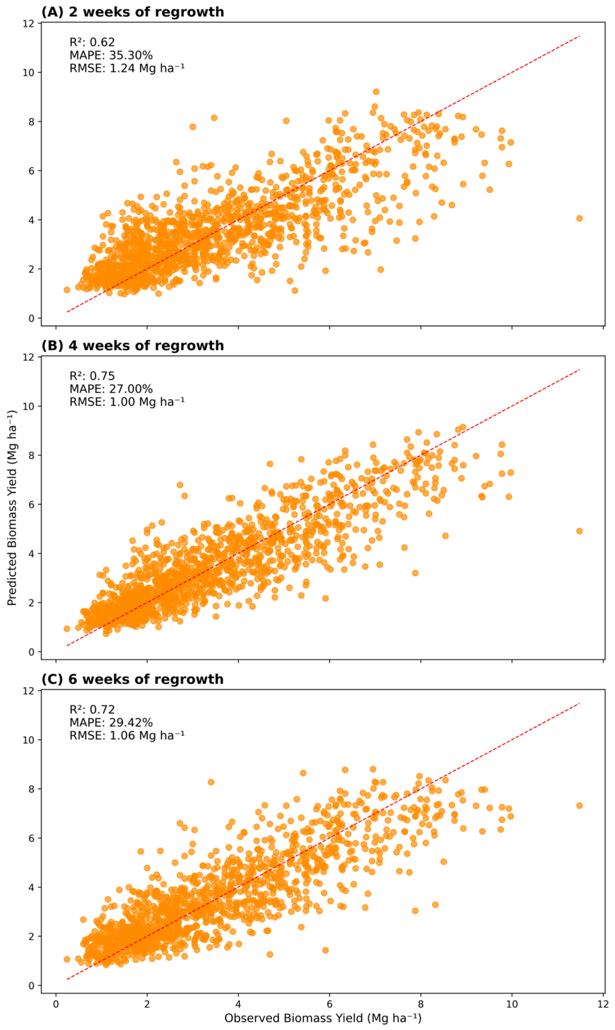
3.1. Non-Cultivar Specific Models

The 2 WOR all-features model (Figure 1A) had the greatest MAPE and RMSE and the least R², meaning it had the greatest error between predicted and observed yield values among all all-features models. Conversely, the 4 WOR all-features model (Figure 1B) showed the least error between predicted and observed values—the least MAPE, RMSE, and the greatest R². Thus, the 6 WOR all-features model (Figure 1C) presented intermediate MAPE, RMSE, and R² (Figure 1).

Although the 4 WOR all-features model was considered the best-performing model, the other developed all-features models presented good yield predictors compared to existing bermudagrass yield models cited in the current literature. For instance, Starks et al. [32] used multi-linear regression analysis to develop different empirical prediction models based on six broad wavebands, such as blue (450–520 nm), green (520–600 nm), red (630–690 nm), NIR (760–900 nm), short-wave infrared 1 (SWIR1, 1550–1750 nm), and short-wave infrared 2 (SWIR2, 2080–2300 nm). The authors’ best bermudagrass prediction model uses the first derivative of reflectance value of 895, 1175, 1975, 2025, and 2235 nm wavelengths, achieving an RMSE and R² of 1.16 Mg ha⁻¹ and 0.63, respectively. In another study, Zhao et al. [33] used multiple regression powered by MAXR (method of maximum R² improvement), achieving an RMSE and R² of 1.02 Mg ha⁻¹ and 0.59, respectively, when combining the reflectance value of 565, 725, 1055, 1215, 1265, 1305, 1465, and 1485 nm wavelengths. Both studies showed bermudagrass prediction models with greater RMSE and lesser R² than our 4 and 6 WOR all-features models and similar to the 2 WOR all-features model. Moreover, Mosali et al. [34] achieved a linear regression R² of 0.41, predicting yield potential in bermudagrass based on a ratio of NDVI values divided by growing degree days where growing degree days were calculated by subtracting the base temperature from the daily average minimum and maximum temperatures.

Moreover, our yield-predicting all-features model performances (R² ranging from 0.62 to 0.75) agreed with existing Random Forest algorithms developed for agricultural purposes. For instance, Zhang et al. [35] achieved an R² of 0.76 by integrating optical, fluorescence, thermal satellite, and environmental data to predict corn yield. Also, the Random Forest algorithm showed improved performance when predicting corn and soybean yield compared to LASSO regression analysis where RF models for corn achieved R² equal to 0.7 and 0.69 for soybean compared to LASSO models for corn and soybean achieving R² of 0.62 and 0.51, respectively [36]; moreover, Jeong et al. [37] found the best RMSE when comparing RF models and multiple linear regression models (MLR) where, when predicting global wheat production, the RMSE for both models was 0.32 and 1.32, respectively; the same trend was observed when predicting corn for grain in the United States (RMSE of 1.13 compared to 1.93), potato in the U.S (RMSE of 2.77 compared to 5.62) and corn for silage (RMSE of 1.9 using RF compared to 4.54 when using MLR).

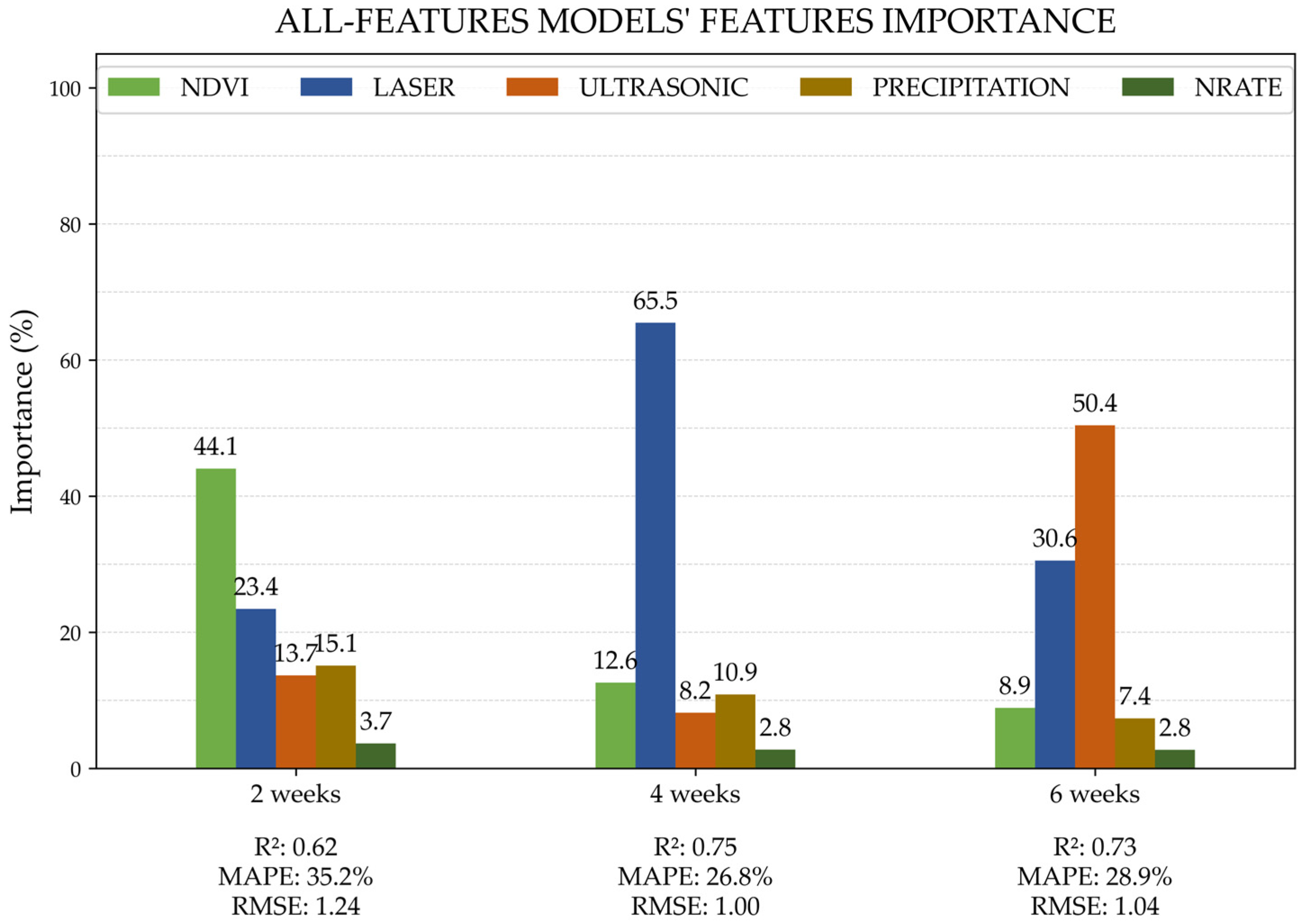
The all-features models trained with data collected at 2, 4, and 6 WOR showed different feature importance score results (Figure 2). Normalized difference vegetation index was the most important feature at 2 WOR followed by laser, precipitation, ultrasonic, and N rate. The NDVI has an elevated performance in yield prediction in early plant development stages when soil exposure is present to contrast with vegetation, increasing the range values of ratios between red and NIR wavelengths [38,39]. Furthermore, since laser and ultrasonic measurements are related to plant height, which did not vary much at bermudagrasses’ early development, NDVI became crucial by reflecting plants’ overall health and vigor.

At 4 WOR, laser became the most important feature, followed by NDVI, precipitation, ultrasonic, and N rate. At this stage, the plants were mid-vegetative, and the canopy was not completely closed [40], allowing the laser to play a key role in assessing height and potential vegetation cover gaps. The laser has a 4.8 mm diameter reading spot that precisely distinguishes bare soil, i.e., “zero”, from canopy height [41].

Conversely, at 6 WOR, the ultrasonic sensor was the most important feature, followed by laser, NDVI, precipitation, and N rate. At this reading event, plant stages varied from late vegetative to anthesis; canopies were denser fully covering the soil (visual inferences only). Ultrasonic sensors capture multiple points within their reading diameter footprint, i.e., 16.61 cm for this experiment (Senix Corporation, 2025), and average them. This average height feature better represents the overall structure and density of the plants when there is less exposed soil due to increased vegetative growth.

After applying the backward feature elimination, most reduced models achieved similar or slightly lower performances than the all-features models.

Table 4. All-features and reduced models after backward feature elimination coefficient of determination (R²), mean absolute percentage error (MAPE), and root mean square error (RMSE) at 2, 4, and 6 weeks of regrowth.

2 Weeks of Regrowth
Features	R2	MAPE (%)	RMSE (Mg ha−1)
NDVI, laser, precipitation, ultrasonic, N rate	0.62	35.18	1.24
NDVI, laser, precipitation, ultrasonic	0.61	35.21	1.25
NDVI, laser, precipitation	0.57	36.01	1.31
NDVI, laser	0.37	43.66	1.59
NDVI	0.36	45.55	1.60
4 Weeks of Regrowth
Features	R2	MAPE (%)	RMSE (Mg ha−1)
Laser, NDVI, precipitation, ultrasonic, N rate	0.75	26.79	1
Laser, NDVI, precipitation, ultrasonic	0.74	27.2	1.02
Laser, NDVI, precipitation	0.72	28.10	1.06
Laser, NDVI	0.60	32.154	1.26
Laser	0.52	37	1.39
6 Weeks of Regrowth
Features	R2	MAPE (%)	RMSE (Mg ha−1)
Ultrasonic, laser, NDVI, precipitation, N rate	0.73	28.91	1.05
Ultrasonic, laser, NDVI, precipitation	0.72	28.84	1.05
Ultrasonic, laser, NDVI	0.63	36.39	1.22
Ultrasonic, laser	0.58	35.36	1.29
Ultrasonic	0.57	36.52	1.31

lists all backward feature elimination for all reading events; however, all feature combinations models’ performance is listed in

Table A1. Coefficient of determination (R²), mean absolute percentage error (MAPE), and root mean square error (RMSE) for features combination when training the model with data collected at two weeks of bermudagrass regrowth.

Features	R2	MAPE (%)	RMSE (Mg ha−1)
NDVI, SONIC, LASER, PRECIPITATION, NRATE	0.62	35.18	1.24
SONIC, LASER, PRECIPITATION, NRATE	0.42	44.84	1.52
NDVI, SONIC, LASER, PRECIPITATION	0.61	35.21	1.25
NDVI, LASER, PRECIPITATION, NRATE	0.60	35.84	1.27
NDVI, SONIC, PRECIPITATION, NRATE	0.56	37.85	1.32
SONIC, LASER, PRECIPITATION	0.42	44.46	1.53
SONIC, PRECIPITATION, NRATE	0.26	50.03	1.72
LASER, PRECIPITATION, NRATE	0.38	47.24	1.58
NDVI, PRECIPITATION, NRATE	0.47	39.86	1.45
NDVI, SONIC, PRECIPITATION	0.54	38.27	1.36
NDVI, LASER, PRECIPITATION	0.57	36.01	1.31
NDVI, SONIC, LASER, NRATE	0.46	41.12	1.48
LASER, PRECIPITATION	0.35	47.30	1.61
SONIC, PRECIPITATION	0.29	49.38	1.70
PRECIPITATION, NRATE	0.26	59.44	1.73
NDVI, PRECIPITATION	0.51	39.12	1.40
SONIC, LASER, NRATE	0.25	51.61	1.73
NDVI, SONIC, LASER	0.43	41.58	1.51
NDVI, LASER, NRATE	0.41	43.03	1.55
NDVI, SONIC, NRATE	0.32	47.13	1.66
PRECIPITATION	0.24	60.43	1.75
SONIC, NRATE	0.06	56.30	1.94
SONIC, LASER	0.22	51.35	1.77
LASER, NRATE	0.16	54.42	1.83
NDVI, NRATE	0.30	46.96	1.67
NDVI, SONIC	0.25	48.50	1.74
NDVI, LASER	0.37	43.66	1.59
LASER	0.16	53.28	1.83
SONIC	0.18	53.70	1.82
NRATE	0.02	69.62	1.99
NDVI	0.36	45.55	1.60

,

Table A2. Coefficient of determination (R²), mean absolute percentage error (MAPE), and root mean square error (RMSE) for features combination when training the model with data collected at four weeks of bermudagrass regrowth.

Features	R2	MAPE (%)	RMSE (Mg ha−1)
NDVI, SONIC, LASER, PRECIPITATION, NRATE	0.75	26.79	1.00
SONIC, LASER, PRECIPITATION, NRATE	0.71	29.83	1.08
NDVI, SONIC, LASER, PRECIPITATION	0.74	27.20	1.02
NDVI, LASER, PRECIPITATION, NRATE	0.73	27.79	1.03
NDVI, SONIC, PRECIPITATION, NRATE	0.70	29.63	1.09
SONIC, LASER, PRECIPITATION	0.70	30.12	1.09
SONIC, PRECIPITATION, NRATE	0.59	35.89	1.28
LASER, PRECIPITATION, NRATE	0.69	31.28	1.12
NDVI, PRECIPITATION, NRATE	0.61	34.10	1.24
NDVI, SONIC, PRECIPITATION	0.68	30.47	1.14
NDVI, LASER, PRECIPITATION	0.72	28.10	1.06
NDVI, SONIC, LASER, NRATE	0.66	30.04	1.17
LASER, PRECIPITATION	0.66	32.45	1.17
SONIC, PRECIPITATION	0.55	37.37	1.34
PRECIPITATION, NRATE	0.26	59.44	1.73
NDVI, PRECIPITATION	0.64	32.29	1.19
SONIC, LASER, NRATE	0.60	33.91	1.26
NDVI, SONIC, LASER	0.65	30.24	1.18
NDVI, LASER, NRATE	0.63	31.52	1.21
NDVI, SONIC, NRATE	0.59	33.80	1.28
PRECIPITATION	0.24	60.43	1.75
SONIC, NRATE	0.43	40.77	1.51
SONIC, LASER	0.59	34.10	1.27
LASER, NRATE	0.53	37.07	1.37
NDVI, NRATE	0.54	36.84	1.35
NDVI, SONIC	0.58	33.93	1.29
NDVI, LASER	0.60	32.15	1.26
LASER	0.52	37.00	1.39
SONIC	0.36	42.21	1.60
NRATE	0.02	69.62	1.99
NDVI	0.59	35.03	1.29

and

Table A3. Coefficient of determination (R²), mean absolute percentage error (MAPE), and root mean square error (RMSE) for features combination when training the model with data collected at six weeks of bermudagrass regrowth.

Features	R2	MAPE (%)	RMSE (Mg ha−1)
NDVI, SONIC, LASER, PRECIPITATION, NRATE	0.73	28.91	1.05
SONIC, LASER, PRECIPITATION, NRATE	0.69	30.76	1.11
NDVI, SONIC, LASER, PRECIPITATION	0.72	28.84	1.05
NDVI, LASER, PRECIPITATION, NRATE	0.69	30.51	1.12
NDVI, SONIC, PRECIPITATION, NRATE	0.69	32.33	1.11
SONIC, LASER, PRECIPITATION	0.69	30.75	1.12
SONIC, PRECIPITATION, NRATE	0.63	36.39	1.22
LASER, PRECIPITATION, NRATE	0.63	32.21	1.22
NDVI, PRECIPITATION, NRATE	0.41	43.91	1.54
NDVI, SONIC, PRECIPITATION	0.68	32.80	1.12
NDVI, LASER, PRECIPITATION	0.67	30.45	1.14
NDVI, SONIC, LASER, NRATE	0.66	31.80	1.16
LASER, PRECIPITATION	0.64	31.19	1.20
SONIC, PRECIPITATION	0.62	35.75	1.24
PRECIPITATION, NRATE	0.26	59.44	1.73
NDVI, PRECIPITATION	0.48	41.23	1.44
SONIC, LASER, NRATE	0.60	34.93	1.27
NDVI, SONIC, LASER	0.65	32.14	1.18
NDVI, LASER, NRATE	0.62	33.73	1.23
NDVI, SONIC, NRATE	0.62	35.22	1.23
PRECIPITATION	0.24	60.43	1.75
SONIC, NRATE	0.53	38.68	1.36
SONIC, LASER	0.58	35.36	1.29
LASER, NRATE	0.56	35.07	1.33
NDVI, NRATE	0.43	43.48	1.51
NDVI, SONIC	0.60	35.96	1.27
NDVI, LASER	0.60	34.32	1.27
LASER	0.61	32.68	1.24
SONIC	0.57	36.52	1.31
NRATE	0.02	69.62	1.99
NDVI	0.49	41.82	1.44

. Backward feature elimination was employed, aiming at a faster processing, simpler, minimalistic algorithm by eliminating less informative features [30,31]. Previous authors used the backward feature elimination procedure, which stated model improvements. Elavarasan et al. [42], when developing prediction models for rice yield using initially 45 features, increased the R² from 0.53 to 0.67 and reduced the MAPE from 21.3% to 19% when implementing an aggregation of the correlation-based filter (CFS) and Random Forest recursive feature elimination (RFRFE). When predicting corn yield using an open-source dataset in Eswatini, Fashoto et al. [43] also observed an increase in the adjusted R² from 0.85 to 0.89 when applying a backward features elimination on an 80–20 training/testing proportion when removing the explanatory variable with the highest p-value.

At 2 WOR, a slight performance decline was observed when eliminating the ultrasonic sensor, followed by an abrupt decline when eliminating the precipitation and laser features.

When the N rate feature was eliminated at 4 WOR, a slight performance decline was observed as well. Then, a minor performance decline was observed with ultrasonic feature elimination, followed by abrupt performance declines when precipitation and NDVI were eliminated.

Likewise, the all-features model performed similarly at the first backward feature elimination at 6 WOR. This model also presented a slight performance decrease when the N rate was eliminated. Then, abrupt performance declines were observed when precipitation, NDVI, and laser were eliminated.

Previous bermudagrass yield prediction models found in the current literature showed R² and RMSE of 0.63 and 1.16 Mg ha⁻¹ [43] and 0.59 and 1.02 Mg ha⁻¹ [33]. Using their performances as a guide, the reduced models containing NDVI, laser, and precipitation features for 2 WOR, laser feature for 4 WOR, and ultrasonic feature for 6 WOR could be considered appropriate.

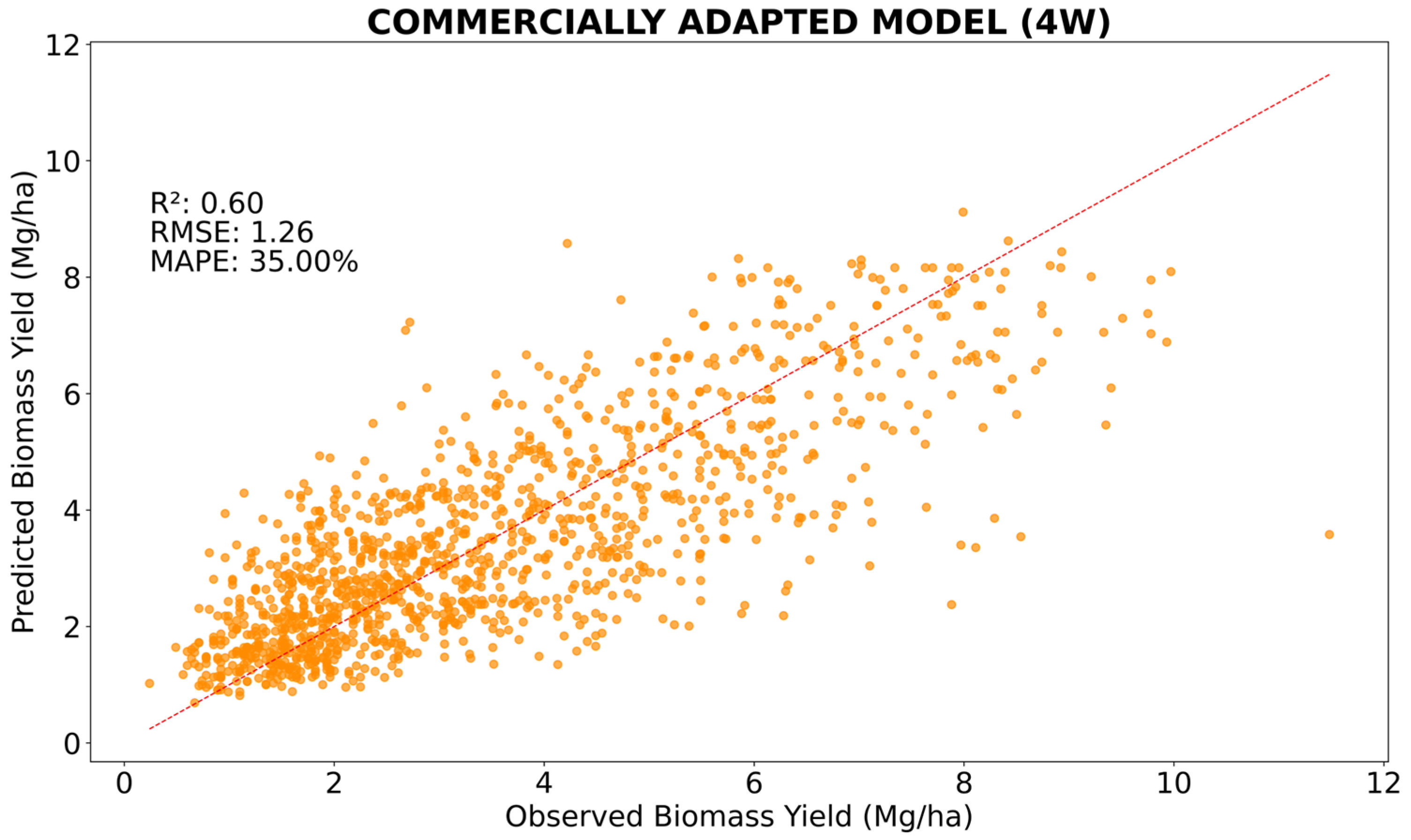
The previously developed bermudagrass yields predictive models used laser and ultrasonic sensors, which are not commonly adopted in commercial forage enterprises. Thus, their uses might be restricted to research development. Thinking about commercial applications, a model was developed using a combination of NDVI, precipitation, and N rate features. Multispectral sensors that allow NDVI calculation are very popular in agricultural enterprises [44,45]. Also, the downside of employing the ultrasonic and laser sensors is that they have 4.3 and 15 m maximum operational distance from the target, respectively, making their use unfeasible on UAVs. This commercially adapted model was developed using readings taken at 4 WOR only because previous models performed best at this reading time.

The commercially adapted model (Figure 3) had an abrupt reduction in its performance (R² decreased from 0.75 to 0.60) compared to the all-features model (Figure 1B). This reduction in performance is related to the removal of the laser feature, which was the feature with the greatest importance (65.5%, Figure 3) at 4 WOR. However, the commercially adapted model showed similar or superior performance to other bermudagrass yield predictive models in the current literature review already cited above [34,35,44].

3.2. Cultivar-Specific Models

Given that 4 WOR readings produced the highest-performing all-features model, and that this sampling time offers a practical balance between prediction accuracy and timely decision making, cultivar-specific models were subsequently developed. This timepoint allows producers to adjust stocking rates or schedule harvests. A model containing all cultivars’ 4 WOR dataset, except Greenfield, was developed as the hay-type cultivars model. A model containing Greenfield, the only grazing-type cultivar [25], dataset was developed, followed by other five cultivars-specific models, such as Goodwell, Midland, Midland 99, Ozark, and Tifton 44. All models are listed in

Table 5. Coefficient of determination (R²), mean absolute percentage error (MAPE), and root mean square error (RMSE) comparison between all-features models and commercially adapted models for the models trained to combine all cultivars, hay-type cultivars, and each cultivar independently.

	All-Features Model			Commercially Adapted Model
	R2	MAPE (%)	RMSE (Mg ha−1)	R2	MAPE (%)	RMSE (Mg ha−1)
All cultivars 1	0.75	26.79	1	0.61	34.1	1.24
Hay-type cultivars 2	0.73	26.05	1.04	0.59	32.21	1.28
Greenfield 3	0.70	28.89	0.80	0.72	27.77	0.77
Goodwell	0.70	24.12	0.96	0.63	28.14	1.04
Midland	0.60	30.31	1.11	0.44	34.11	1.33
Midland99	0.75	26.35	1.03	0.66	30.42	1.20
Ozark	0.74	24.88	1.03	0.66	26.40	1.17
Tifton44	0.64	28.41	1.07	0.52	31.59	1.22

¹ Goodwell, Greenfield, Midland99, Midland, Ozark, and Tifton44 cultivars combined. ² Goodwell, Midland99, Midland, Ozark, and Tifton44 cultivars combined. ³ Grazing cultivar.

.

When comparing the all-features model trained with all cultivars (R², MAPE, and RMSE of 0.75, 26.79, and 1.0, respectively) to all cultivar-specific and hay-type cultivars models, only the cultivar-specific model for Midland99 and Ozark had the same or slightly reduced performance compared to the model trained with all cultivars. Cultivars-specific models for Greenfield, Tifton 44, Goodwell, and hay-type cultivars had reduced performance compared to the model trained with all cultivars. Moreover, the Midland cultivar-specific model had an abrupt performance decline compared to the model trained with all cultivars.

A different scenario was found when comparing the commercially adapted model trained with all cultivars (R², MAPE, and RMSE of 0.61, 34.1, and 1.24, respectively) to cultivar-specific and hay-type cultivar models. Greenfield, Midland 99, and Ozark had considerable improvement in performance, whereas Goodwell had a slight improvement. The association of hay-type cultivars and Tifton 44 showed a declined performance, and Midland showed an abrupt decline.

All-cultivars, hay-type, and cultivar-specific models built with all features showed higher performance than the commercially adapted ones. This result reinforced the information displayed in Figure 2, where the laser was the most important feature (i.e., 65.5%) in all-features, all-cultivar models at 4 WOR. Thus, its removal led to a decline in model performance in most commercially adapted models, such as the all-cultivars model, the hay-type cultivar model, Midland 99, Tifton 44, Midland, Ozark, and Goodwell.

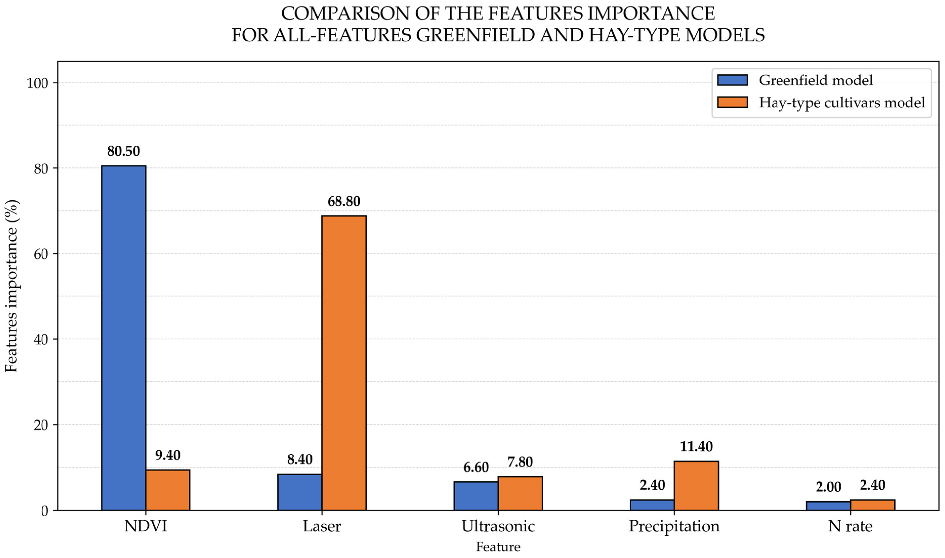
Nevertheless, the Greenfield commercially adapted cultivar model showed a slight increase in its performance when compared to the Greenfield all-features model presenting R², MAPE, and RMSE changes of +0.02, −1.12 percent units, and −0.03 Mg ha⁻¹, respectively. Further features importance examination presented in Figure 4 revealed that the Greenfield all-features model’s most important input was NDVI (80.50%) followed by laser (68.80%), ultrasonic (7.80%), precipitation (11.40%), and N rate (2.0%). This result differed from the all-features hay-type model, which showed laser as the most important feature (68.80%) followed by precipitation (11.40%), NDVI (9.40%), ultrasonic (7.80%), and N rate (2.40).

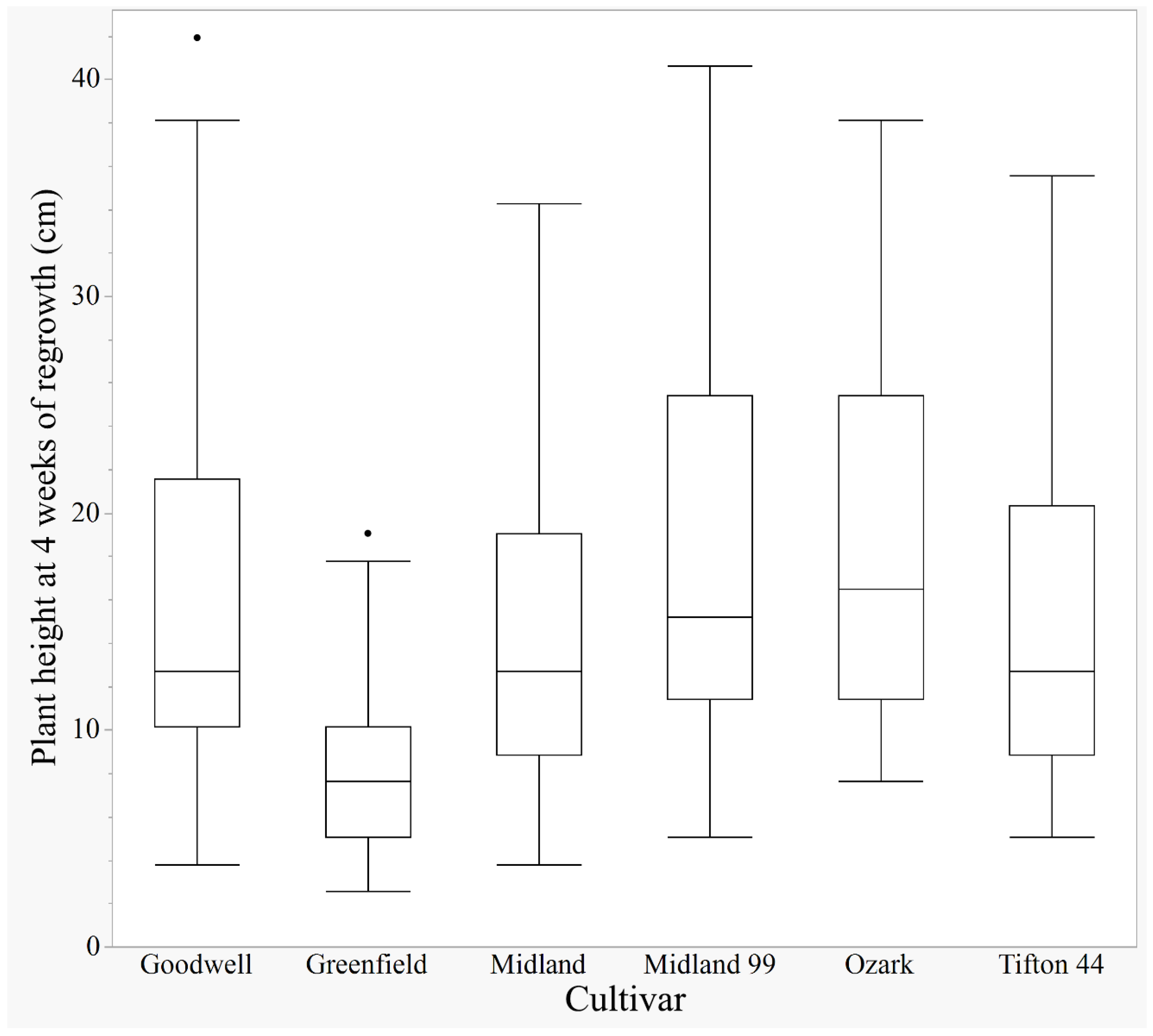
The Greenfield cultivar is short and creeping, and its average height is statistically lower (13.8 cm) than that of all the other hay cultivars (19.5–25 cm) used in this experiment (Figure A1). Thus, Greenfield did not benefit from the height measurements provided by laser and ultrasonic; otherwise, it mostly benefited from NDVI, which reflects the overall health and vigor of the plants at 4 WOR.

4. Conclusions

After Random Forest training and validating all possible features, reading events, and cultivars combinations, the all-features model developed with 4 WOR readings showed the highest performance (R² = 0.75, MAPE = 26.79%, RMSE = 1.0 Mg ha⁻¹) with the laser proximity sensor having the highest feature importance score (65.5%), followed by NDVI (12.6%), precipitation (10.9%), ultrasonic (8.2%), and N rate (2.8%). However, the all-features model developed with 6 and 2 WOR readings performed better than the existing bermudagrass biomass predicting models in the current literature (R² ≥ 0.62, RMSE ≤ 1.24 Mg ha⁻¹). Furthermore, the simplified version of the all-features model developed with 4 WOR readings, in which N rate and ultrasonic features were backward-eliminated, also showed superior performance compared to the existing models in the literature. Finally, unlike proximity sensors, multispectral sensors are widely adopted in agricultural enterprises. Then, a commercially adapted model, including only the multispectral sensor, precipitation, and N rate features at 4 WOR, outperformed the previously developed models and the existing models in the literature. Thus, the Random Forest regressor, proximity, and multispectral sensors showed strong potential as tools for developing effortless and efficient models to predict bermudagrass biomass yield accurately at different nitrogen application rates. However, the present model was trained and validated under Oklahoma environmental conditions only. Further re-training and validation might be necessary to extend the present model’s applicability to other environmental conditions. Finally, the model could benefit from the addition of other soil and management practices-based training features which might increase the model’s generalization.

References

1. Peel, D.S. Beef cattle growing and backgrounding programs. Vet. Clin. Food Anim. Pract. 2003, 19, 365–385. [Google Scholar] [CrossRef] [PubMed]
2. Rao, S.C.; Coleman, S.W.; Mayeux, H.S. Forage production and nutritive value of selected pigeonpea ecotypes in the southern great plains. Crop Sci. 2002, 42, 1259–1263. [Google Scholar] [CrossRef]
3. Evers, G.W.; Parsons, M.J. Temperature influence on seeded bermudagrass germination. Tex. J. Agric. Nat. Resour. 2009, 22, 74–80. [Google Scholar]
4. Collins, M.; Nelson, C.J.; Moore, K.J.; Barnes, R.F. Forages, Volume 1: An Introduction to Grassland Agriculture, 7th ed.; John Wiley & Sons: Hoboken, NJ, USA, 2017. [Google Scholar]
5. Schneider-Canny, R.; Chekhovskiy, K.; Munoz, P.; Kwon, S.; Saha, M.C. Characterization of bermudagrass (Cynodon dactylon L.) germplasm for nitrogen use efficiency. Euphytica 2019, 215, 40. [Google Scholar] [CrossRef]
6. Arnall, B.; Jones, J.J.; Pugh, B.; Rocateli, A.; Sanders, H.; Warren, J.; Zhang, H. Oklahoma Forage and Pasture Fertility Guide; Oklahoma State University: Stillwater, OK, USA, 2018. [Google Scholar]
7. Nielsen-Gammon, J.W.; Zhang, F.; Odins, A.M.; Myoung, B. Extreme rainfall in Texas: Patterns and predictability. Phys. Geogr. 2005, 26, 340–364. [Google Scholar] [CrossRef]
8. Horn, K.M.; Rocateli, A.C.; Warren, J.G.; Turner, K.E.; Antonangelo, J.A. Introducing grazeable cover crops to the winter wheat systems in Oklahoma. Agron. J. 2020, 112, 3677–3694. [Google Scholar] [CrossRef]
9. Rocateli, A.; Freires Abreu, L. Oklahoma Bermudagrass Variety Performance Tests: 2019 Forage Year; Oklahoma State University: Stillwater, OK, USA, 2020. [Google Scholar]
10. Rocateli, A. Plan Grazing Management Using the Oklahoma Grazing Stick; Oklahoma State University: Stillwater, OK, USA, 2016. [Google Scholar]
11. Harmoney, K.R.; Moore, K.J.; George, J.R.; Brummer, E.C.; Russell, J.R. Determination of pasture biomass using four indirect methods. Agron. J. 1997, 89, 665–672. [Google Scholar] [CrossRef]
12. Martin, R.C.; Astatkie, T.; Cooper, J.M.; Fredeen, A.H. A comparison of methods used to determine biomass on naturalized swards. J. Agron. Crop Sci. 2005, 191, 152–160. [Google Scholar] [CrossRef]
13. Woli, P.; Rouquette Jr, F.M.; Long, C.R.; Gowda, P.; Pequeno, D.N. Simulated Bermudagrass Production and Nitrate Leaching Affected by El Niño-Southern Oscillation, Soil, and Clipping Frequency. Agron. J. 2017, 109, 2649–2661. [Google Scholar] [CrossRef]
14. Woli, P.; Rouquette, F.M., Jr.; Long, C.R. Investigating DSSAT: Bermudagrass response to nitrogen as influenced by soil and climate. Agron. J. 2019, 111, 1741–1751. [Google Scholar] [CrossRef]
15. Chlingaryan, A.; Sukkarieh, S.; Whelan, B. Machine learning approaches for crop yield prediction and nitrogen status estimation in precision agriculture: A review. Comput. Electron. Agric. 2018, 151, 61–69. [Google Scholar] [CrossRef]
16. Van Klompenburg, T.; Kassahun, A.; Catal, C. Crop yield prediction using machine learning: A systematic literature review. Comput. Electron. Agric. 2020, 177, 105709. [Google Scholar] [CrossRef]
17. Pittman, J.J.; Arnall, D.B.; Interrante, S.M.; Moffet, C.A.; Butler, T.J. Estimation of biomass and canopy height in bermudagrass, alfalfa, and wheat using ultrasonic, laser, and spectral sensors. Sensors 2015, 15, 2920–2943. [Google Scholar] [CrossRef] [PubMed]
18. Pantazi, X.E.; Moshou, D.; Alexandridis, T.; Whetton, R.L.; Mouazen, A.M. Wheat yield prediction using machine learning and advanced sensing techniques. Comput. Electron. Agric. 2016, 121, 57–65. [Google Scholar] [CrossRef]
19. Rehman, T.U.; Mahmud, M.S.; Chang, Y.K.; Jin, J.; Shin, J. Current and future applications of statistical machine learning algorithms for agricultural machine vision systems. Comput. Electron. Agric. 2019, 156, 585–605. [Google Scholar] [CrossRef]
20. Elavarasan, D.; Vincent, D.R.; Sharma, V.; Zomaya, A.Y.; Srinivasan, K. Forecasting yield by integrating agrarian factors and machine learning models: A survey. Comput. Electron. Agric. 2018, 155, 257–282. [Google Scholar] [CrossRef]
21. Rashid, M.; Bari, B.S.; Yusup, Y.; Kamaruddin, M.A.; Khan, N. A comprehensive review of crop yield prediction using machine learning approaches with special emphasis on palm oil yield prediction. IEEE Access 2021, 9, 63406–63439. [Google Scholar] [CrossRef]
22. Karthickmanoj, R.; Sasilatha, T.; Singh, N.S.S. Plant Disease Detection Using Random Forest Classifier with Novel Segmentation and Feature Extraction Strategy. J. Eng. Sci. Technol. Spec. Issue ICIT2022 2023, 18, 32–38. [Google Scholar]
23. Carranza, C.; Nolet, C.; Pezij, M.; van der Ploeg, M. Root zone soil moisture estimation with Random Forest. J. Hydrol. 2021, 593, 125840. [Google Scholar] [CrossRef]
24. Breiman, L. Random forests. Mach. Learn. 2001, 45, 5–32. [Google Scholar] [CrossRef]
25. Abreu, L.F.; Rocateli, A.C. Selecting an Appropriate Bermudagrass Variety for Pastures. In Oklahoma Cooperative Extension; Oklahoma State University: Stillwater, OK, USA, 2019; Available online: http://dasnr22.dasnr.okstate.edu/docushare/dsweb/Get/Document-11354/PSS-2600web.pdf (accessed on 31 January 2024).
26. McKinney, W. pandas: A foundational Python library for data analysis and statistics. Python High Perform. Sci. Comput. 2011, 14, 1–9. [Google Scholar]
27. Pedregosa, F.; Varoquaux, G.; Gramfort, A.; Michel, V.; Thirion, B.; Grisel, O.; Blondel, M.; Prettenhofer, P.; Weiss, R.; Dubourg, V.; et al. Scikit-learn: Machine learning in Python. J. Mach. Learn. Res. 2011, 12, 2825–2830. [Google Scholar]
28. Scikit-Learn Developers. Scikit-Learn: Machine Learning in Python (Version 1.4.1) [Software]; Scikit-Learn.org, 2023A. Available online: https://scikit-learn.org (accessed on 15 February 2024).
29. Scikit-Learn Developers. Random Forest Classifier. In Scikit-Learn: Machine Learning in Python, 2023B. Available online: https://scikitlearn.org/stable/modules/generated/sklearn.ensemble.RandomForestClassifier.html (accessed on 15 February 2024).
30. Sharif, M.; Khan, M.A.; Iqbal, Z.; Azam, M.F.; Lali, M.I.U.; Javed, M.Y. Detection and classification of citrus diseases in agriculture based on optimized weighted segmentation and feature selection. Comput. Electron. Agric. 2018, 150, 220–234. [Google Scholar] [CrossRef]
31. Jiang, Y.; Li, C. mRMR-based feature selection for classification of cotton foreign matter using hyperspectral imaging. Comput. Electron. Agric. 2015, 119, 191–200. [Google Scholar] [CrossRef]
32. Starks, P.J.; Zhao, D.; Phillips, W.A.; Coleman, S.W. Development of canopy reflectance algorithms for real-time prediction of bermudagrass pasture biomass and nutritive values. Crop Sci. 2006, 46, 927–934. [Google Scholar] [CrossRef]
33. Zhao, D.; Starks, P.J.; Brown, M.A.; Phillips, W.A.; Coleman, S.W. Assessment of forage biomass and quality parameters of bermudagrass using proximal sensing of pasture canopy reflectance. Grassl. Sci. 2007, 53, 39–49. [Google Scholar] [CrossRef]
34. Mosali, J.; Girma, K.; Teal, R.K.; Freeman, K.W.; Raun, W.R. Use of In-Season Reflectance for Predicting Yield Potential in Bermudagrass. Commun. Soil Sci. Plant Anal. 2007, 38, 1519–1531. [Google Scholar] [CrossRef]
35. Zhang, L.; Zhang, Z.; Luo, Y.; Cao, J.; Tao, F. Combining optical, fluorescence, thermal satellite, and environmental data to predict county-level maize yield in China using machine learning approaches. Remote Sens. 2019, 12, 21. [Google Scholar] [CrossRef]
36. Khaki, S.; Wang, L.; Archontoulis, S.V. A CNN-RNN framework for crop yield prediction. Front. Plant Sci. 2020, 10, 492736. [Google Scholar] [CrossRef]
37. Jeong, J.H.; Resop, J.P.; Mueller, N.D.; Fleisher, D.H.; Yun, K.; Butler, E.E.; Kim, S.H. Random forests for global and regional crop yield predictions. PLoS ONE 2016, 11, e0156571. [Google Scholar] [CrossRef]
38. Freeman, K.W.; Girma, K.; Arnall, D.B.; Mullen, R.W.; Martin, K.L.; Teal, R.K.; Raun, W.R. By-plant prediction of corn forage biomass and nitrogen uptake at various growth stages using remote sensing and plant height. Agron. J. 2007, 99, 530–536. [Google Scholar] [CrossRef]
39. Marti, J.; Bort, J.; Slafer, G.A.; Araus, J.L. Can wheat yield be assessed by early measurements of Normalized Difference Vegetation Index? Ann. Appl. Biol. 2007, 150, 253–257. [Google Scholar] [CrossRef]
40. de Campos Jezus, G.C.; Rocateli, A.C. Development of Sensor-Based Bermudagrass (Cynodon dactylon L. Pers.) Yield and Crude Protein Prediction Models in Eastern Oklahoma. In Proceedings of the 2023 ASA-CSSA-SSSA International Annual Meeting, Saint Louis, MO, USA, 29 October–1 November 2023. [Google Scholar]
41. Balogh, R. Evaluation of the optoncdt ilr sensor. 2014; Unpublished work. [Google Scholar]
42. Elavarasan, D.; Vincent, P.M.; Srinivasan, K.; Chang, C.Y. A hybrid CFS filter and RF-RFE wrapper-based feature extraction for enhanced agricultural crop yield prediction modeling. Agriculture 2020, 10, 400. [Google Scholar] [CrossRef]
43. Fashoto, S.G.; Mbunge, E.; Ogunleye, G.; van den Burg, J. Implementation of machine learning for predicting maize crop yields using multiple linear regression and backward elimination. Malays. J. Comput. 2021, 6, 679–697. [Google Scholar] [CrossRef]
44. U.S. Geological Survey. NDVI, the Foundation for Remote Sensing Phenology. 2018. Available online: https://www.usgs.gov/special-topics/remote-sensing-phenology/science/ndvi-foundation-remote-sensing-phenology (accessed on 18 January 2024).
45. Huang, S.; Tang, L.; Hupy, J.P.; Wang, Y.; Shao, G. A commentary review on the use of normalized difference vegetation index (NDVI) in the era of popular remote sensing. J. For. Res. 2021, 32, 1–6. [Google Scholar] [CrossRef]
Figure 1. All-features models’ scatterplots contrasting the observed and predicted biomass yield (Mg ha−1), and presenting the coefficient of determination (R2), mean absolute percentage error (MAPE), and root mean square error (RMSE) at 2 (A), 4 (B), and 6 (C) weeks of regrowth. The orange dots represent each observation point.
Agronomy 15 01004 g001
Figure 2. All-features models’ features importance for 2, 4, and 6 weeks of bermudagrass regrowth.
Agronomy 15 01004 g002
Figure 3. Commercially adapted model scatterplots contrasting the observed and predicted biomass yield (Mg ha−1), and presenting the coefficient of determination (R2), mean absolute percentage error (MAPE), and root mean square error (RMSE) at 4 weeks of regrowth.
Agronomy 15 01004 g003
Figure 4. Comparison of the feature’s importance for the all-features Greenfield and hay-type models.
Agronomy 15 01004 g004