Article

Development of Mathematical and Computational Models for Predicting Agricultural Soil–Water Management Properties (ASWMPs) to Optimize Intelligent Irrigation Systems and Enhance Crop Resilience

by
Brigitta Tóth
1,*,
Oswaldo Guerrero-Bustamante
2,*,
Michel Murillo
2,
Jose Duque
2 and
Rodrigo Polo-Mendoza
3
1
Institute of Food Science, Faculty of Agricultural and Food Sciences and Environmental Management, University of Debrecen, Böszörményi Str. 138, H-4032 Debrecen, Hungary
2
Department of Civil and Environmental, Universidad de la Costa, Barranquilla 080003, Colombia
3
Department of Civil and Environmental Engineering, Universidad del Norte, Barranquilla 081007, Colombia
*
Authors to whom correspondence should be addressed.
Agronomy 2025, 15(4), 942; https://doi.org/10.3390/agronomy15040942
Submission received: 7 March 2025 / Revised: 28 March 2025 / Accepted: 11 April 2025 / Published: 12 April 2025

Abstract

:
Soil–water management is fundamental to plant ecophysiology, directly affecting plant resilience under both anthropogenic and natural stresses. Understanding Agricultural Soil–Water Management Properties (ASWMPs) is therefore essential for optimizing water availability, enhancing harvest resilience, and enabling informed decision-making in intelligent irrigation systems, particularly in the face of climate variability and soil degradation. In this regard, the present research develops predictive models for ASWMPs based on the grain size distribution and dry bulk density of soils, integrating both traditional mathematical approaches and advanced computational techniques. By examining 900 soil samples from the NaneSoil database, spanning diverse crop species (Avena sativa L., Daucus carota L., Hordeum vulgare L., Medicago sativa L., Phaseolus vulgaris L., Sorghum vulgare Pers., Triticum aestivum L., and Zea mays L.), several predictive models are proposed for three key ASWMPs: soil-saturated hydraulic conductivity, field capacity, and permanent wilting point. Mathematical models demonstrate high accuracy (71.7–96.4%) and serve as practical agronomic tools but are limited in capturing complex soil–plant-water interactions. Meanwhile, a Deep Neural Network (DNN)-based model significantly enhances predictive performance (91.4–99.7% accuracy) by uncovering nonlinear relationships that govern soil moisture retention and plant water availability. These findings contribute to precision agriculture by providing robust tools for soil–water management, ultimately supporting plant resilience against environmental challenges such as drought, salinization, and soil compaction.

1. Introduction

Crop water stress materializes when plants receive insufficient water to meet their physiological needs, negatively affecting growth, development, and yield [1,2]. This deficiency in water supply can be caused by drought, excessive evapotranspiration, poor soil water retention, or inefficient irrigation practices [3,4]. Most vegetable crops are highly sensitive to water stress, particularly in the 2–3 weeks before harvest and during the harvest itself, which can induce an irreversible loss of yield or product quality [1,5,6]. The preceding highlights the necessity of designing irrigation water management plans to optimize intelligent irrigation systems and enhance crop resilience [7,8,9]. In order to develop these plans, it is essential to have a detailed knowledge of the Agricultural Soil–Water Management Properties (ASWMPs).
ASWMPs can be defined as a set of physical parameters that describe the capacity of soils to retain, transmit, and supply water to crops within the framework of smart irrigation systems [10,11,12,13]. Hence, properly characterizing ASWMPs is fundamental to ensuring the sustainability and cost-efficiency of field crops. Among the key ASWMPs, three are particularly important: Soil Saturated Hydraulic Conductivity (SSHC), Field Capacity (FC), and Permanent Wilting Point (PWP). Unfortunately, the comprehensive mapping of soil hydraulic properties remains economically unfeasible in many resource-limited agricultural regions [14,15,16,17,18,19], such as sub-Saharan Africa, rural India, Southeast Asia, the Andean Highlands, the Sahel Region, Central America, and the Middle East. Therefore, it is crucial to conceive indirect methods to predict ASWMPs that can be easily implemented using only basic soil characterization [20,21]. Precisely, this study proposes several mathematical and computational models to estimate three meaningful ASWMPs, namely SSHC, FC, and PWP.
On the one hand, SSHC is a velocity-like quantity that defines a soil’s ability to conduct water through its porous structure when fully saturated (i.e., when the degree of saturation is equal to 1) [22,23]. Meanwhile, FC represents the water content that soil can retain after undergoing saturation, followed by gravity-induced drainage, typically occurring two to three days after rainfall or irrigation [24,25]. On the other hand, PWP refers to the moisture level within the soil matrix that plants can no longer effectively absorb, leading to wilting [26,27]. Figure 1 illustrates the graphical representation of the fully saturated state, FC, and PWP. Measuring these ASWMPs in a large-scale agricultural practice presents significant challenges due to soil complexity and the numerous factors influencing its hydraulic behaviour [7,28,29]. Previous research has widely discussed the importance and difficulty of field and laboratory measurements for SSHC, FC, and PWP [30,31,32]. Given these challenges, there is an opportunity to develop indirect methods to estimate ASWMPs based on fundamental soil properties.
Accordingly, this study aims to propose robust mathematical and computational models for predicting SSHC, FC, and PWP within applications in agricultural engineering. The proposed models use Dry Bulk Density (DBD) and grain size composition (i.e., sand, silt, and clay contents) as input variables, which cultivators can easily determine at minimal expense. Thus, this investigation seeks to empower agriculturists to adopt precision irrigation and management strategies even under substantial budget constraints, thereby reducing resource waste and promoting sustainable agribusiness practices.
The remainder of this paper is structured as follows. Section 2 describes the adopted database and the characteristics of the analyzed soil samples. Section 3 outlines the development of mathematical and computational models based on statistical correlations and Deep Neural Networks (DNNs), respectively. Subsequently, Section 4 assesses the precision and performance of these models. Then, Section 5 presents a detailed discussion of the primary advantages and challenges associated with the proposed models. It outlines their key benefits, identifies potential limitations, and explores the implications for practical applications in the field. Finally, Section 6 summarizes the research findings and key conclusions.

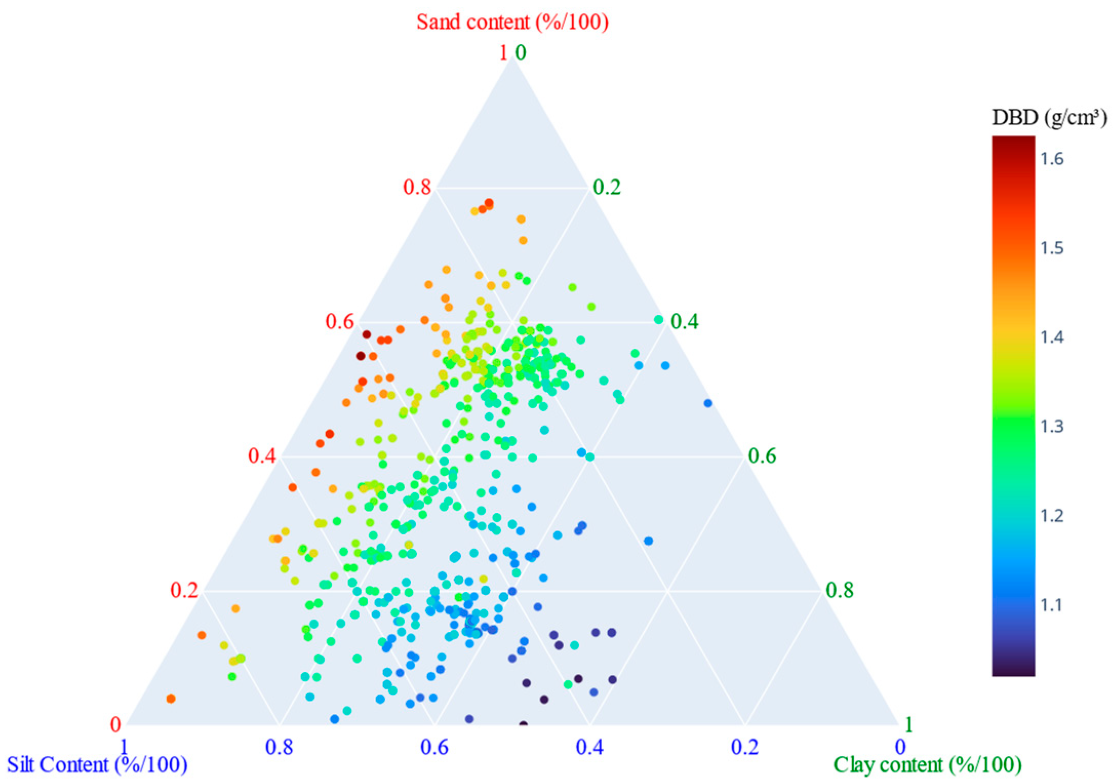
2. Data Source

This study utilized the NaneSoil database to develop mathematical and computational models for predicting three ASWMPs: SSHC, FC, and PWP. This open database was published in 2023 [34]. The previously mentioned research, along with [21,35,36], provides detailed information on data collection. NaneSoil contains 900 records detailing the experimental characterization of agricultural soils in San Juan del Río (Querétaro, Mexico). Table 1 classifies these soil samples based on soil texture and cultivated crops, while Figure 2 presents a ternary plot illustrating the grain size distribution of the analyzed soil samples.
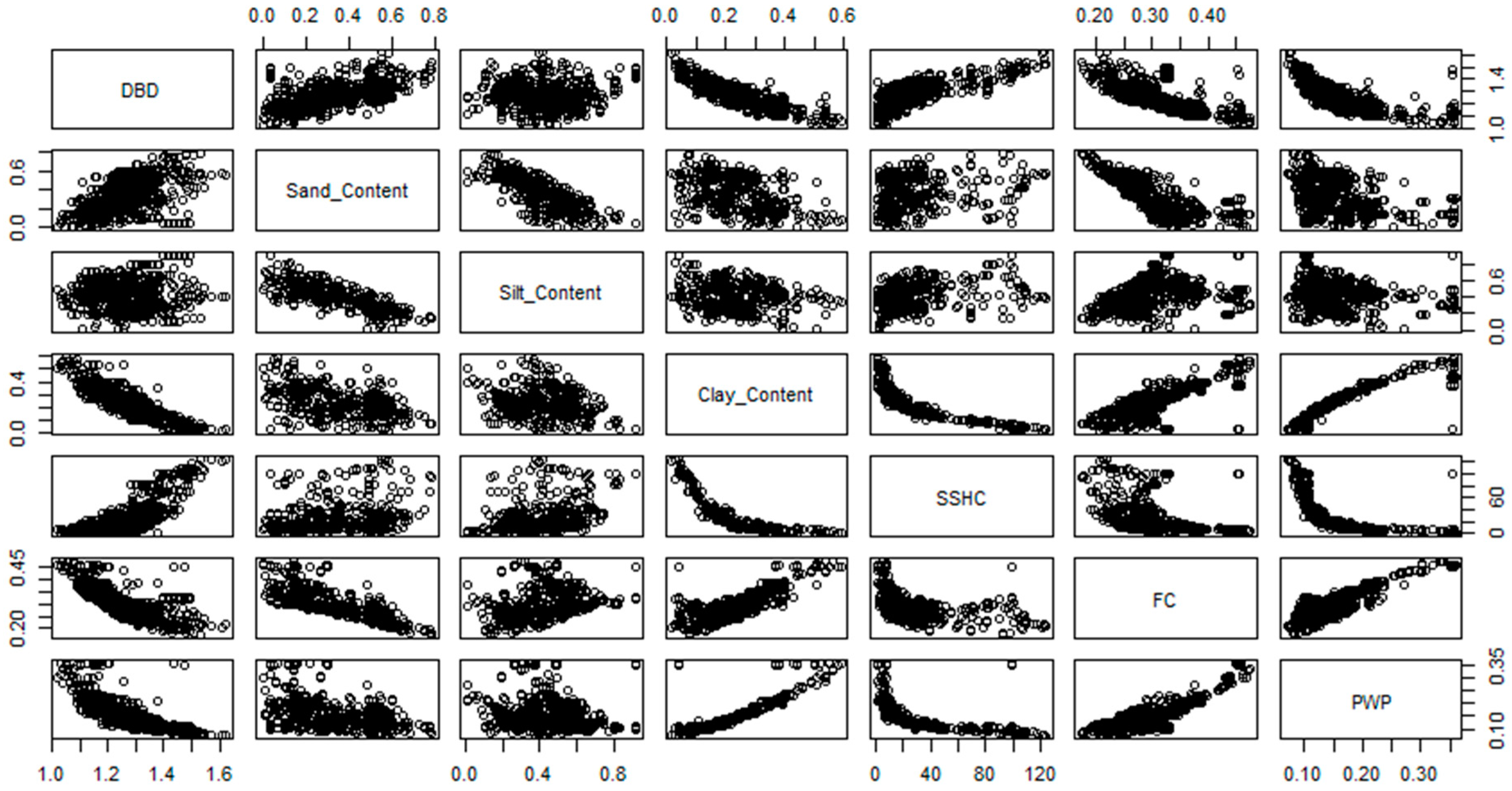
According to Table 1 and Figure 2, the NaneSoil database covers a wide variety of grain size distributions, from fine-grained soils (e.g., clay and silt) to predominantly granular soils (e.g., loam and sandy loam). Further insights into the database can be found in Figure 3, which shows a scatterplot matrix of the selected variables, i.e., four input variables and three output variables. The input variables correspond to the DBD and the grain size composition (sand, silt, and clay contents), while the output variables correspond to three ASWMPs: SSHC, FC, and PWP. Figure 3 reveals strong correlations between several of the input and output variables: (i) DBD and SSHC, (ii) clay content and SSHC, (iii) clay content and FC, and (iv) clay content and PWP. These findings suggest that DBD and the clay content are the most significant input variables, whereas sand and silt contents exhibit a weaker direct relationship with ASWMPs.

3. Methods

This research employs two types of methods to develop predictive models of ASWMPs, namely mathematical and computational modelling. On the one hand, mathematical modelling is based on statistical correlations. On the other hand, the computation modelling is focused on a specific Machine Learning (ML)-based technique called Artificial Neural Networks (ANNs). These methods are described in detail below.

3.1. Mathematical Modelling

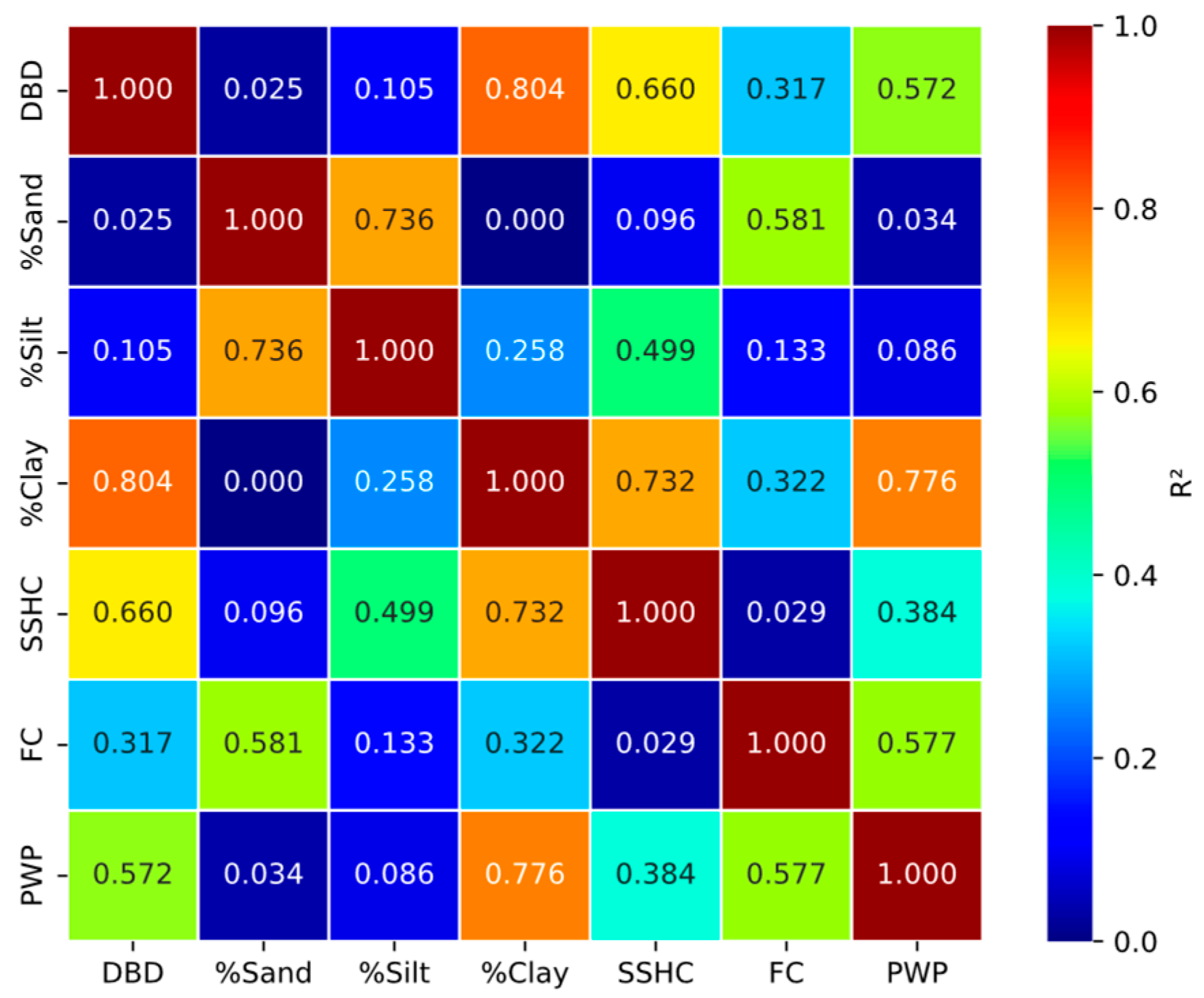
In order to establish mathematical correlations between the input variables (i.e., DBD, sand content, silt content, and clay content) and output variables (i.e., SSHC, FC, and PWP), it is necessary to analyze the dependence between each variable and the others. While Figure 3 presents initial findings, further examination is required. In order to support this, Figure 4 displays a heatmap illustrating the dependence between variables, showing the coefficient of determination (R2) for these relationships.
The heatmap in Figure 4 confirms that the three ASWMPs studied correlate highly with the DBD and clay content. It is important to highlight that clay content stands out as the most influential input variable. In this regard, it is worth a more in-depth inspection of the relationships between variables described in Figure 3. These results are shown later in the manuscript.

3.2. Computational Modelling

Although mathematical models can be very accurate, they may not be robust enough to describe non-obvious relationships between variables. Moreover, mathematical models are weak in terms of adaptability because they rely on fixed equations and predefined assumptions (e.g., linearity or homogeneity). Once formulated, mathematical models are often static and struggle to accommodate new data, changing conditions, or unexpected complexities. Fortunately, ML-based techniques can easily overcome these limitations and significantly improve the precision of models (i.e., compared to classical statistical correlations) [37,38].
Initially, it is essential to demarcate what ML is. Although there is no consensus in the literature, it is possible to provide a definition widely accepted by the engineering and scientific communities. In this regard, ML is the branch of artificial intelligence that focuses on developing statistic-based algorithms that enable computers to learn from data and subsequently generate predictions, inferences, or decisions [39,40,41]. Within the broad set of ML algorithms for regression problems, it is possible to mention the decision trees, random forest regression, gradient boosting machines, support vector regression, and Artificial Neural Networks [42,43,44].
This research uses ANNs to predict three ASWMPs (i.e., SSHC, FC, and PWP). ANNs are computational models inspired by the human brain, designed to recognize patterns and solve complex problems thanks to their capability to generalize from instances/samples [45,46]. ANNs consist of layers of interconnected nodes (i.e., the so-called neurons) that process data through weighted connections and activation functions [47,48]. ANNs learn by adjusting these weights based on input data along the epochs (i.e., the training-and-testing cycles) [49,50]. This study employs a specific type of ANN, namely Deep Neural Networks (DNNs). The DNNs are characterized by having at least two hidden layers with densely connected neurons, allowing them to capture intricate relationships within data [38,51]. The design of the computational architecture and the performance of the proposed DNN-based model are presented later in the manuscript.

4. Results

4.1. Statistical Correlations

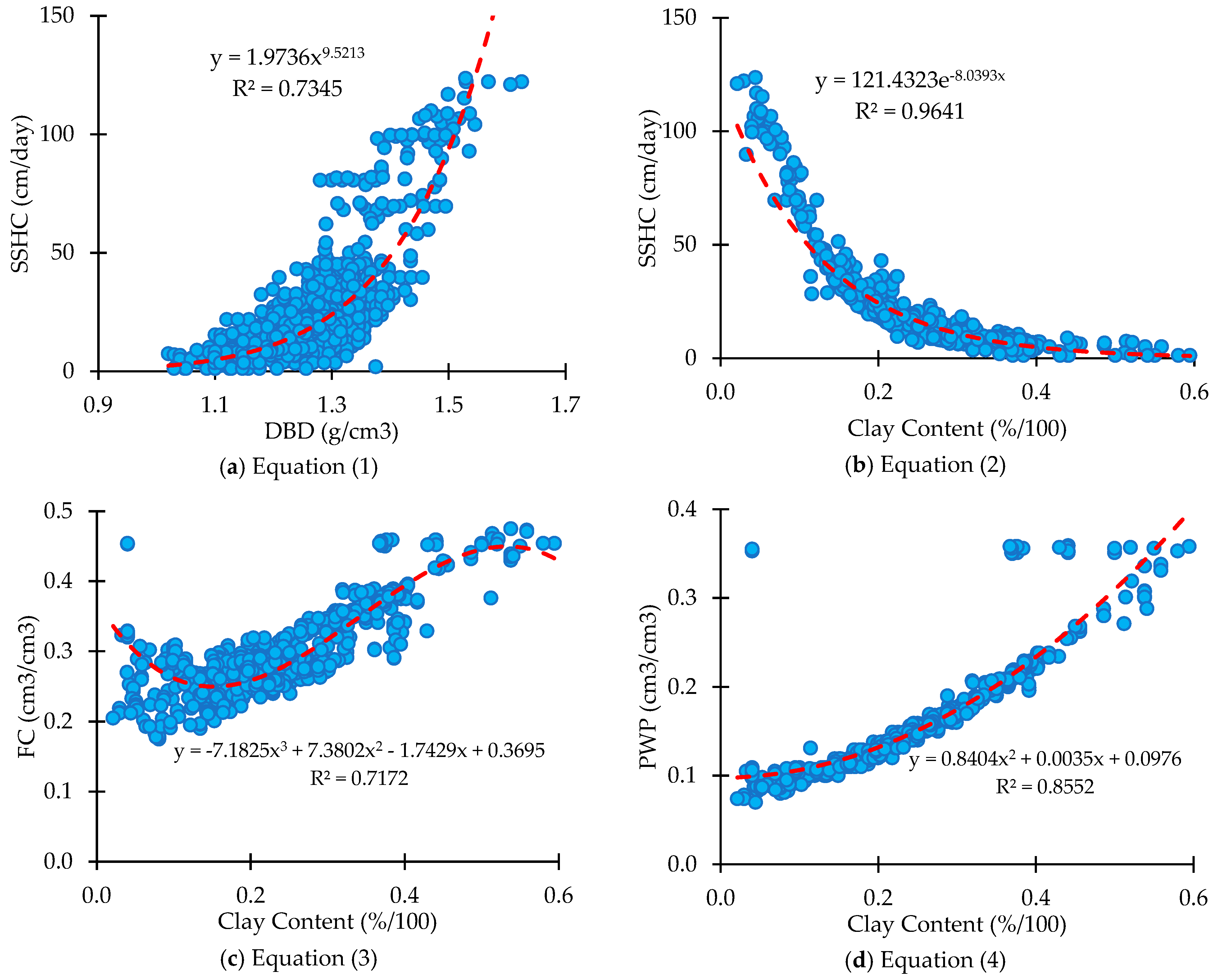
The previously mentioned correlations between the input and output variables are stated in Equation (1) (DBD vs. SSHC), Equation (2) (clay content vs. SSHC), Equation (3) (clay content vs. FC), and Equation (4) (clay content vs. PWP). Based on R2, these equations demonstrate predictive accuracy of 73.45%, 96.41%, 71.72%, and 85.52%, respectively. Figure 5 shows a graphic representation of these mathematical models, highlighting that SSHC and PWP can be predicted with high accuracy using Equations (2) and (4). However, FC predictions could benefit from a more refined model. Therefore, an additional correlation is introduced in Equation (5), which is validated through statistical tests (Student’s t and F-tests) in Table 2. This equation estimates FC based on DBD and grain size distribution (sand, silt, and clay contents) and achieves an adjusted R2 value of 0.9106, indicating high precision.
S S H C = 1.9736   D B D 9.5213
S S H C = 121.4323   e 8.0393   c l a y
F C = 7.1825   c l a y 3 + 7.3802   c l a y 2 1.7429   c l a y + 0.3695
P W P = 0.8404   c l a y 2 + 0.0035   c l a y + 0.0976
F C = 0.2351 + 0.2803   l n D B D + 1 0.5122   ln s a n d + 1 0.2374   ln s i l t + 1 + 0.2891   ln c l a y + 1
where
SSHC is expressed in cm/day;
FC and PWP are expressed in cm3/cm3;
DBD is expressed in g/cm3;
sand, silt, clay are the sand content, silt content, and clay content, respectively. All are expressed in %/100.

4.2. Artificial Neural Network

Mathematical models in Equations (1)–(5) show significantly high accuracy and can serve as reliable tools for preliminary estimates in daily agricultural engineering practices. Nonetheless, advanced computational models offer even greater predictive accuracy. In order to enhance precision, this study also proposes a DNN-based model to simultaneously predict SSHC, FC, and PWP. For this purpose, it is necessary to start by applying data pre-processing techniques.
Table 3 presents the basic statistical description (minimum, maximum, mean, median, standard deviation, kurtosis, and skewness) of the variables obtained from the NaneSoil database. Table 3 shows that these variables present diverse units and order of magnitudes. This scenario can yield a challenging learning process, even avoiding the convergence of several ML models [37,52,53]. Consequently, it was decided to perform a data processing technique named feature scaling. In order to address this, feature scaling was applied using Equation (6) [54,55], the so-called min-max scaling with a target range of [−1, 1]. This transformation standardizes all variables, rendering them dimensionless and ensuring that all values fall within the specific range [41,56]. The main advantage of this procedure is that all the transformed variables lose their units and become dimensionless quantities. Also, all the data records are between the specified range (i.e., from −1 to 1). Table 4 summarizes the statistical description of the scaled dataset, confirming that mean, median, and standard deviation values remain within the expected range (between −1 and +1). Notably, kurtosis and skewness values did not change after scaling, indicating that the transformation preserves the original data distribution and does not mitigate the effect of outliers.
X s c a l e d = X o r i g i n a l X m i n X m a x X m i n T a r g e t m a x T a r g e t m i n + T a r g e t m i n
where
X s c a l e d represents a scaled data point between a specific range;
X o r i g i n a l represents a data point on the original scale;
X m i n is the minimum value (of a variable) within the adopted data records;
X m a x is the maximum value (of a variable) within the adopted data records;
T a r g e t m i n is the minimum value specified for the scaling range. In this case, −1;
T a r g e t m a x is the maximum value specified for the scaling range. In this case, 1.
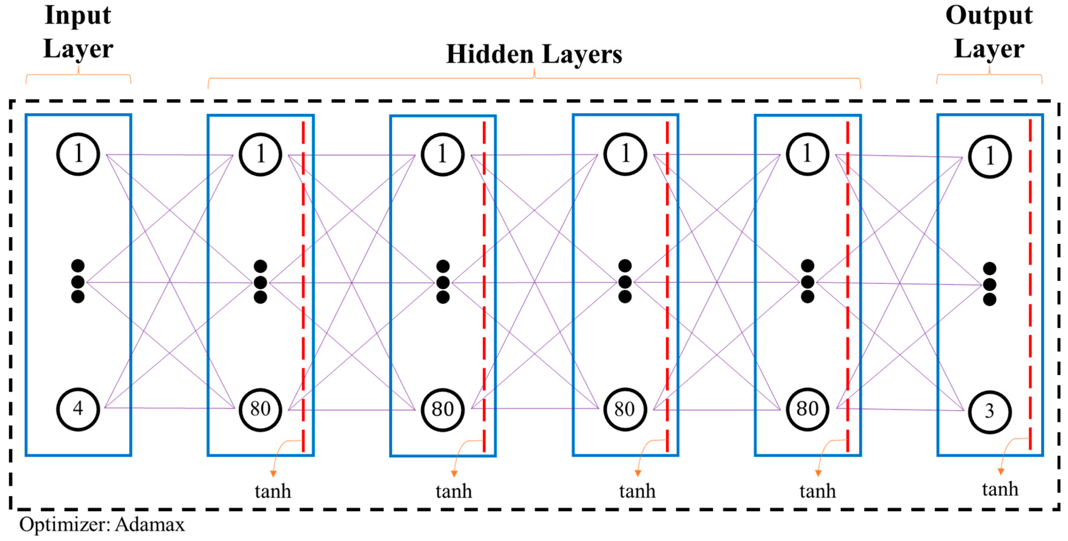
After the feature scaling, the 900 data records were divided into three datasets: (i) training dataset: 80% for (720 records), (ii) testing dataset: 10% (90 records), and (iii) validation dataset: 10% (90 records). For this study, the DNN’s input layer comprises four neurons, i.e., one for each input variable (DBD, sand content, silt content, and clay content). The output layer consists of three neurons corresponding to the three ASWMPs (SSHC, FC, and PWP). The number of hidden layers and neurons was determined through a trial-and-error process, resulting in the architecture presented in Figure 6. According to this graph, the designed DNN has four hidden layers, each with 80 neurons. Therefore, this computational model is composed of 20,083 trainable parameters. Table 5 explains the process of calculating the number of trainable parameters.
In Figure 6, it is evident that the proposed DNN model has two main characteristics. The tangent hyperbolic (tanh) activation function is applied to the hidden and output layers. This activation function was deliberately included because it yields all the outgoing values of a layer to be located within the closed range between −1 and 1 [57,58], which is particularly desired in this case study due to the feature scaling previously introduced. The Adamax algorithm is used as the optimization method. Adamax, a robust first-order gradient-based optimizer, that uses the concept of exponentially weighted infinity norm and Exponential Decay Rate (EDR) to modify the learning rate based on data characteristics [59,60]. Table 6 shows a detailed explanation of this optimizer and the hyperparameter values used in this study.

4.2.1. Model’s Precision

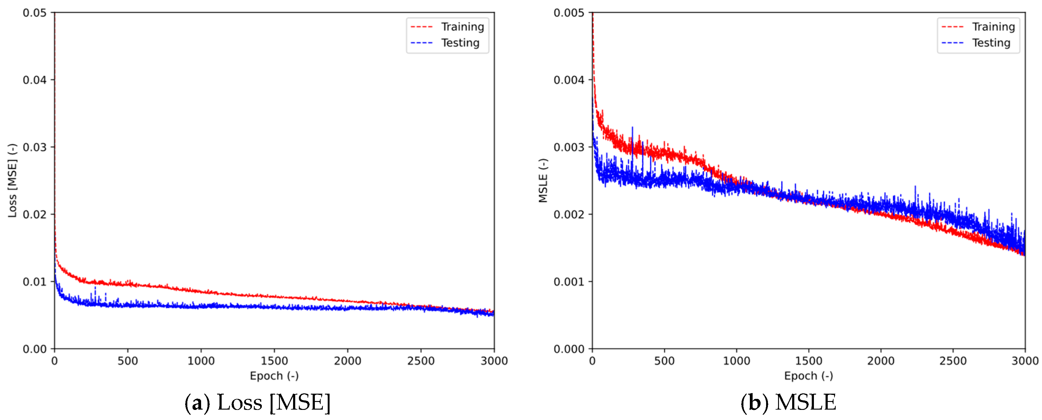
The proposed model required 3000 epochs. This number of training-and-testing cycles was determined using the early stopping technique over the adopted loss function, i.e., Mean Squared Error (MSE, Equation (7)). Figure 7 illustrates the evolution of the loss function along with an additional error metric, the Mean Squared Logarithmic Error (MSLE, Equation (8)), over the epochs. In addition, the model’s precision was evaluated using five goodness-of-fit parameters: R2 and four error metrics. These error metrics include the MSE, MSLE, Mean Absolute Error (MAE, Equation (9)), and Mean Absolute Percentage Error (MAPE, Equation (10)) [37,38,51]. These results are presented in Table 7. According to this table, the forecasting errors associated with the proposed DNN model are minimal after 3000 epochs. Moreover, the R2 values indicate that the computational model can estimate SSHC, FC, and PWP with accuracies ranging from 98.7% to 99.7%, 97.4% to 97.8%, and 91.4% to 94.0%, respectively. This accuracy is further evidenced in Figure 8 through 1:1 lines.
M S E = 1 m i = 1 m O D i E D i 2
M S L E = 1 m i = 1 m l n ( 1 + O D i ) l n ( 1 + E D i ) 2
M A E = 1 m i = 1 m O D i E D i
M A P E = 1 m i = 1 m O D i E D i O D i
where
m is the number of addressed data records;
i is the data index;
ODi is an original/experimental data point;
EDi is an estimated data point.

4.2.2. Model’s Explainability

ML-based models, especially deep learning models (i.e., the ones built on ANNs), often function as black boxes, meaning their internal decision-making processes are complex and complicated to interpret [62,63]. While most DNN architectures can be represented as mathematical functions, explicitly writing them out is impractical (in most cases) due to the sheer number of parameters, even tens of thousands in the simplest models [64,65]. The preceding leads to the performance of explainability analysis that permits to infer the internal functioning of ML models. This research employs SHapley Additive exPlanations (SHAP) and partial dependence assessments for this purpose.
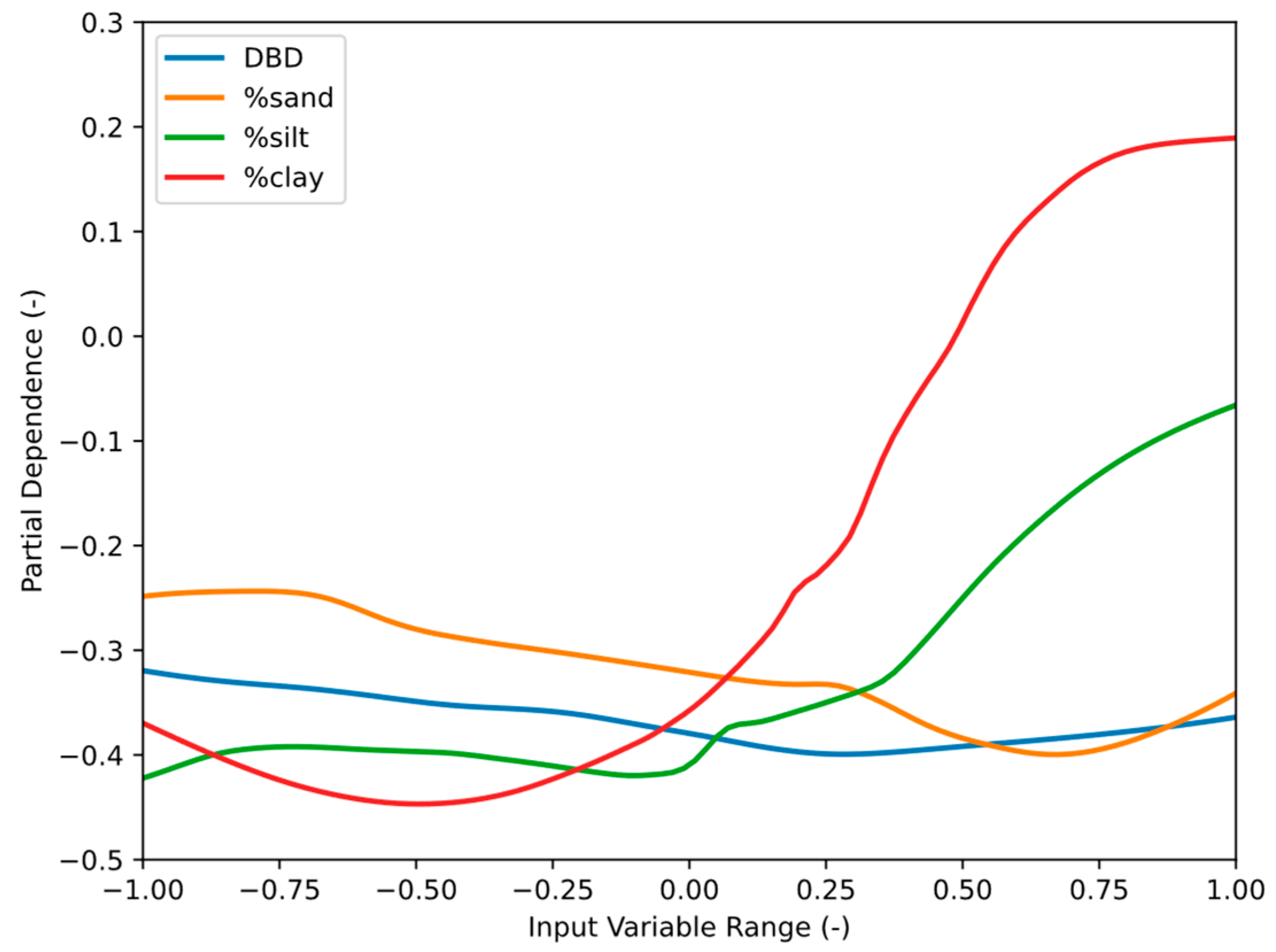
On the one hand, a Partial Dependence Plot (PDP) is shown in Figure 9. PDPs display the effect of each input variable on a model’s predictions while averaging out the effects of other variables [66,67]. In other words, the PDPs help to understand how the input variables affect the average response of the addressed model [68,69]. Generally, steeper curves with more remarkable changes indicate a greater dependence between that input variable and the set of output variables [70,71]. Accordingly, the following findings can be drawn from Figure 9:
  • The clay content has the strongest effect, with a sharp rise, suggesting a strong positive impact on predictions at higher values. The preceding is consistent with the findings discovered in Figure 3, Figure 4 and Figure 5. These graphs showed that clay content is highly correlated with all output variables, and there is a general upward trend between the clay content and two ASWMPs (i.e., FC and PWP).
  • The silt content follows a pattern similar to that of clay but with a less pronounced effect. Initially, the silt content shows a decreasing trend, but over time, it begins to rise. This suggests that the model’s output also increases as the silt content augments. Likewise, these results are congruent with Figure 3, where it is clear that there is a general upward trend between the silt content and two ASWMPs (i.e., SSHC and FC).
  • The sand content exhibits a mild, oscillating effect, suggesting it moderately influences predictions. The preceding agrees with Figure 4. Regardless, the sand content undergoes a general downward trend, suggesting that the model’s output decreases as the sand content augments. This dependency was previously observed in Figure 3, where two ASWMPs (i.e., FC and PWP) diminished at higher sand content values.
  • Finally, DBD shows a relatively stable effect with a slight falling pattern. This behaviour agrees with previous results in Figure 3 and Figure 4, where it is notorious that DBD has a moderate influence on the output variables and has a general downward trend with two ASWMPs (i.e., FC and PWP).
On the other hand, SHAP analysis is presented in Figure 10. SHAP analysis, derived from game theory, is a technique widely used to interpret ML models [37,72,73]. It quantifies the contribution of each input variable to the model’s outputs by distributing the prediction difference fairly among all input features, helping to explain how the model works [74,75,76]. Nevertheless, it is important to highlight that SHAP results are sensitive to slight modifications in model architecture and hyperparameter tuning [73,77,78]. In order to provide insights into the proposed DNN’s decision-making process, two SHAP interpretations were conducted, namely a summary bar plot (see Figure 10a) and a summary beeswarm plot (see Figure 10b). Below are the findings that can be drawn from Figure 10.
In the bar plot (see Figure 10a), SHAP values indicate the mean influence of input variables on output variables [37,78]. The most influential variables, ranked in descending order of importance, are clay content, sand content, silt content, and, finally, DBD. This ranking indicates that clay content has the strongest impact on the model’s predictions, followed by sand and silt content, while DBD has the least influence among these variables. Notably, these results align with the patterns observed in the PDP, reinforcing the consistency of the model’s behaviour and feature interactions. It is also interesting to emphasize that although DBD alone is sufficient to estimate SSHC (see Equation (1) and Figure 5a), it is the less important variable in the overall model response. The preceding can be attributed to the fact that DNN is trained to predict all three ASWMPs simultaneously. As a result, the model must balance the influence of each input variable across multiple outputs rather than a single one. This leads to a second key insight, i.e., ANNs can reveal hidden relationships between variables that may not be apparent through traditional statistical approaches, highlighting their ability to capture complex interactions within the data [42,44,47].
In the beeswarm plot (see Figure 10b), each point represents a SHAP value for a particular data instance, with colour indicating feature magnitude (blue for low and red for high values) [79,80,81]. The results from this analysis and the PDP show some similarities but also key discrepancies in how the input variables describe feature importance and influence on model output. Both plots suggest that the clay and silt contents have a notable impact on predictions, but they reveal different insights into how these features contribute. The beeswarm plot captures local feature importance, displaying how individual instances (with varying feature values) impact model predictions. It highlights that the silt content tends to have a negative effect, while the other input variables have both positive and negative impacts depending on their values. The PDP, in contrast, provides a global perspective by showing the average marginal effect of each feature on predictions. It indicates that the clay content has a strong nonlinear influence, becoming more positive at higher values, whereas the silt content also trends positively at higher values. These disparities arise because SHAP values account for interactions between features in individual predictions, while PDP isolates each feature’s effect by averaging over all other feature values. This means that the beeswarm plot can capture complex interactions that PDP may not, explaining why tendencies observed in the two plots can differ.

4.2.3. Model’s Efficiency

When analyzing the efficiency of ANN-based models, two key factors are execution time and memory consumption [82,83]. Execution time refers to the duration required to train the model, which is influenced by factors such as network depth, layer complexity, and hardware acceleration [84,85]. Meanwhile, memory consumption refers to the amount of Random-Access Memory (RAM) needed to store model parameters, activations, and gradients during the learning process [86,87]. Higher RAM usage can slow down processing or even cause crashes if the system lacks sufficient memory [88,89].
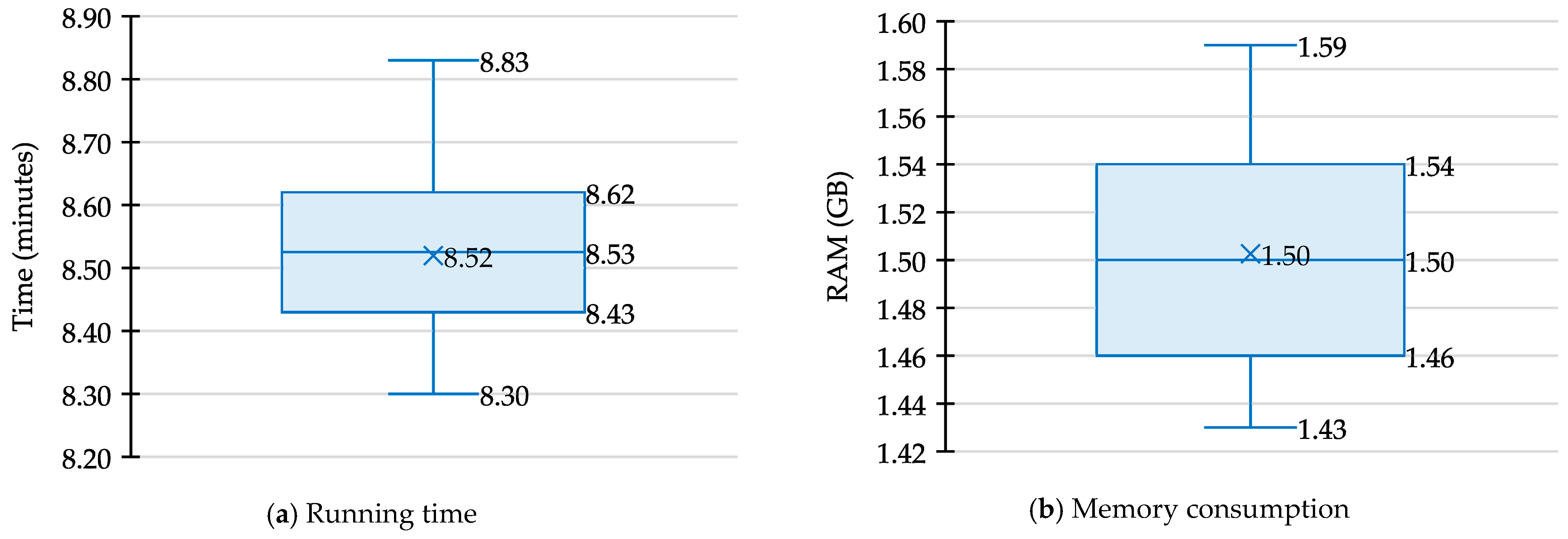
These efficiency analyses do not provide insights into the accuracy of the results but rather the willingness of potential users to adopt new computational models. High execution times or elevated RAM consumption may discourage potential users, leading them to favour traditional mathematical models that are easier to implement. This research employs Python’s native modules “TIME” and the external library “PSUTIL” to determine the runtime and RAM usage, respectively. In order to ensure reliability, 100 independent runs were performed, with the results presented in Figure 11 through box-and-whisker plots. Thus, the average running time and memory consumption were 8.52 min and 1.50 GB, respectively. These results indicate moderate resource usage, making it convenient for systems with typical memory capacities. Overall, these results demonstrate that the proposed DNN model strikes a suitable balance between performance and resource efficiency, making it accessible to a wide range of potential users.
It is crucial to note that the outcomes of these assessments are influenced by both software and hardware specifications [37,38]. Therefore, to ensure transparency, the computational resources used in this study are detailed as follows: Google Colab 1.2.0 (a cloud-based Jupyter Notebook service) was employed as the development environment, while an NVIDIA® Tesla T4 GPU was used as acceleration hardware.

4.2.4. Model’s Generalizability

K-fold cross-validation is a robust technique for assessing a model’s generalizability by systematically partitioning the dataset into K subsets, or folds, ensuring that each data point is used for both training and testing [90,91]. This approach mitigates bias and variance by iteratively training the model on K−1 folds while evaluating its performance on the remaining fold, averaging the results across all iterations [92,93]. K-fold cross-validation comprehensively estimates the model’s predictive capability on unseen data by preventing overfitting to a specific data partition [94,95].
In this research, a five-fold cross-validation analysis was conducted on 900 data records from the Nanesoil database to assess the generalizability of the proposed DNN and ensure that its performance was not the result of multiple overfitting occurrences. Thus, for this five-fold cross-validation process, the 900 data records were randomly partitioned into five equal subsets of 180 records each. In each iteration, the proposed DNN was trained on four subsets (i.e., a total of 720 data records) and tested on the remaining one, ensuring that every data point was considered in the procedure.
Figure 12 shows the results of the k-fold cross-validation on the loss function. As seen in this graph, the training and testing datasets evolve properly along the 3000 epochs for all the folds, which implies that the proposed DNN model does not suffer from overfitting. In this regard, potential users are free to choose either of the two learning approaches employed in this study (i.e., train-test split or k-fold cross-validation) depending on their specific application and validation needs. Regardless of the preferred approach, both alternatives have been demonstrated to produce consistently high-accuracy results, ensuring reliable model performance.

4.2.5. Comparison Versus Automatic ML-Based Models

Finally, comparing the proposed DNN model against an automatic ML-based framework is essential to evaluate its performance, robustness, and practical applicability. Thus, the H2O AutoML was adopted for comparative purposes [96]. H2O AutoML provides an automated pipeline that selects and tunes multiple ML models, optimizing them without requiring extensive user intervention [96,97,98]. By benchmarking the proposed DNN against this state-of-the-art automated framework, it is possible to assess whether the tailored designed architecture offers competitive advantages in terms of accuracy.
By executing H2O AutoML on the Nanesoil database, this framework evaluated 20 different ML models spanning several methods. As a result of this implementation, it was determined that the most accurate algorithm was a stacked ensemble model, which in turn combines multiple base models (i.e., gradient boosting machines, extreme gradient boosting, ANNs, and distributed random forests) using a generalized linear model as the metalearner.
The prediction results on the validation dataset obtained from this model are exhibited in Figure 13. It was chosen to show the results for this dataset because it is the most critical, as it represents data never before known by the model. As can be visually observed, the H2O AutoML framework was highly accurate, yielding R2 values of 0.9839 for the SSHC, 0.9717 for the FC, and 0.9305 for the PWP. This level of exactness is slightly lower than that associated with the proposed DNN model (see Table 7).
In this regard, such a comparison highlights the strengths and potential limitations of both approaches, offering valuable insights into the advantages of domain-specific DNN customization over general-purpose automated modelling. Given that the H2O AutoML framework demonstrated high accuracy yet still slightly underperformed compared to the proposed DNN, this evaluation reinforces the practical significance of a tailored deep learning approach. It ensures that the proposed model is not only theoretically robust but also superior in predictive accuracy, making it highly relevant for real-world applications.

5. Discussion

First and foremost, it is important to highlight that the analysis of 900 soil samples from the NaneSoil database, which includes a diverse range of soil textures, provides valuable insights into the relationships between basic soil characterization and ASWMPs. This diverse sample set ensured a comprehensive representation of soil types commonly encountered in agricultural settings. By analyzing the relationships between the fundamental physical properties of soil and the three output variables (i.e., SSHC, FC, and PWP), five mathematical correlations (Equations (1)–(5)) and one DNN architecture (see Figure 6) were developed. These models demonstrated high accuracy, making them suitable for preliminary estimations in agricultural engineering practices, particularly in the design and assessment of intelligent irrigation systems.

5.1. Comparison of the Proposed Models

It is essential to highlight that the proposed DNN-based model is designed to predict SSHC, FC, and PWP simultaneously. The R2 values for the forecasts ranged from 98.7% to 99.7% for SSHC, 97.4% to 97.8% for FC, and 91.4% to 94.0% for PWP. Overall, this level of precision surpasses that of the proposed mathematical models (71.7–96.4%) and effectively captures more complex relationships between variables, which classical statistical correlations fail to explain. These results indicate that the DNN model accurately estimates ASWMPs, capturing a significant portion of the data’s variance and providing precise estimations. The minimal forecasting errors and high R2 values further demonstrate the reliability of the developed model. Its high accuracy suggests that it can be effectively utilized for informed decision-making in agricultural soil–water management practices. Thus, the use of ML techniques, such as ANNs, offers a promising approach for improving the accuracy and precision of ASWMP predictions, potentially leading to optimized agricultural practices and improved resource management strategies.
PDP and SHAP analysis were conducted in order to obtain insights into the explainability and interpretability of the proposed DNN model. These assessments revealed that, although the developed DNN exhibits certain computing patterns similar to those of the introduced correlations, the influence of specific input variables on the output variables is less explicit. This is primarily due to the simultaneous calculation of all output variables in the DNN, which obscures simpler relationships that are more evident in mathematical models. Overall, these findings highlight the complex relationships between the studied ASWMPs (i.e., SSHC, FC, and PWP) and the fundamental physical properties of soils (i.e., grain size distribution and DBD), emphasizing the importance of considering advanced computational models to enhance ASWMP prediction.
SSHC, FC, and PWP are essential parameters for hydrological and agronomic research [32,99]. Empirical and theoretical studies have shown that FC, PWP, and SSHC positively correlate with clay content [24,100], which agrees with this investigation. However, DNN models have occasionally identified contradictory negative correlations. This discrepancy is likely due to implicit correlations, nonlinear feature interactions, data biases, and the absence of physical constraints in DNN models. Additionally, mathematical formulations can sometimes be restricted by factors such as computational limitations, complexity, usability, data quality and uncertainty, and the suitability of model parameterizations [38,101]. In this regard, future studies should consider hybrid modelling approaches integrating ML-based techniques with physical knowledge to improve model accuracy and interpretability.

5.2. Limitations of the Study

The main limitation of this study is the exclusion of organic carbon content as an input variable due to the lack of this information in the NaneSoil database. This omission is significant because organic carbon is a key determinant of soil structure, porosity, and water retention, all of which strongly influence ASWMPs [102,103,104,105]. Its absence may impact the accuracy and applicability of the predictive models, particularly in soils with elevated organic matter content. Additionally, the study relies solely on the grain size distribution and DBD to estimate ASWMPs, overlooking other critical factors such as soil mineralogy, aggregation, and biological activity, which also regulate soil–water interactions. The NaneSoil database, while extensive, may not fully capture the diversity of soil types, climatic conditions, and agricultural practices worldwide, potentially limiting the generalizability of the models.
Furthermore, although the proposed DNN-based model enhances predictive accuracy by capturing nonlinear relationships, it does not fully account for dynamic soil–plant-water interactions, which are crucial for real-world applications. Lastly, the interpretability of ML models remains a challenge, as their complexity can obscure the underlying drivers of ASWMP estimations, making it difficult for soil scientists and agronomists to derive actionable insights. In this regard, future research should address these limitations by incorporating organic carbon data, expanding the dataset to cover a broader range of soil conditions, and integrating additional soil properties to enhance both the precision and practical utility of ASWMP prognostic models.

5.3. Real-World Applications

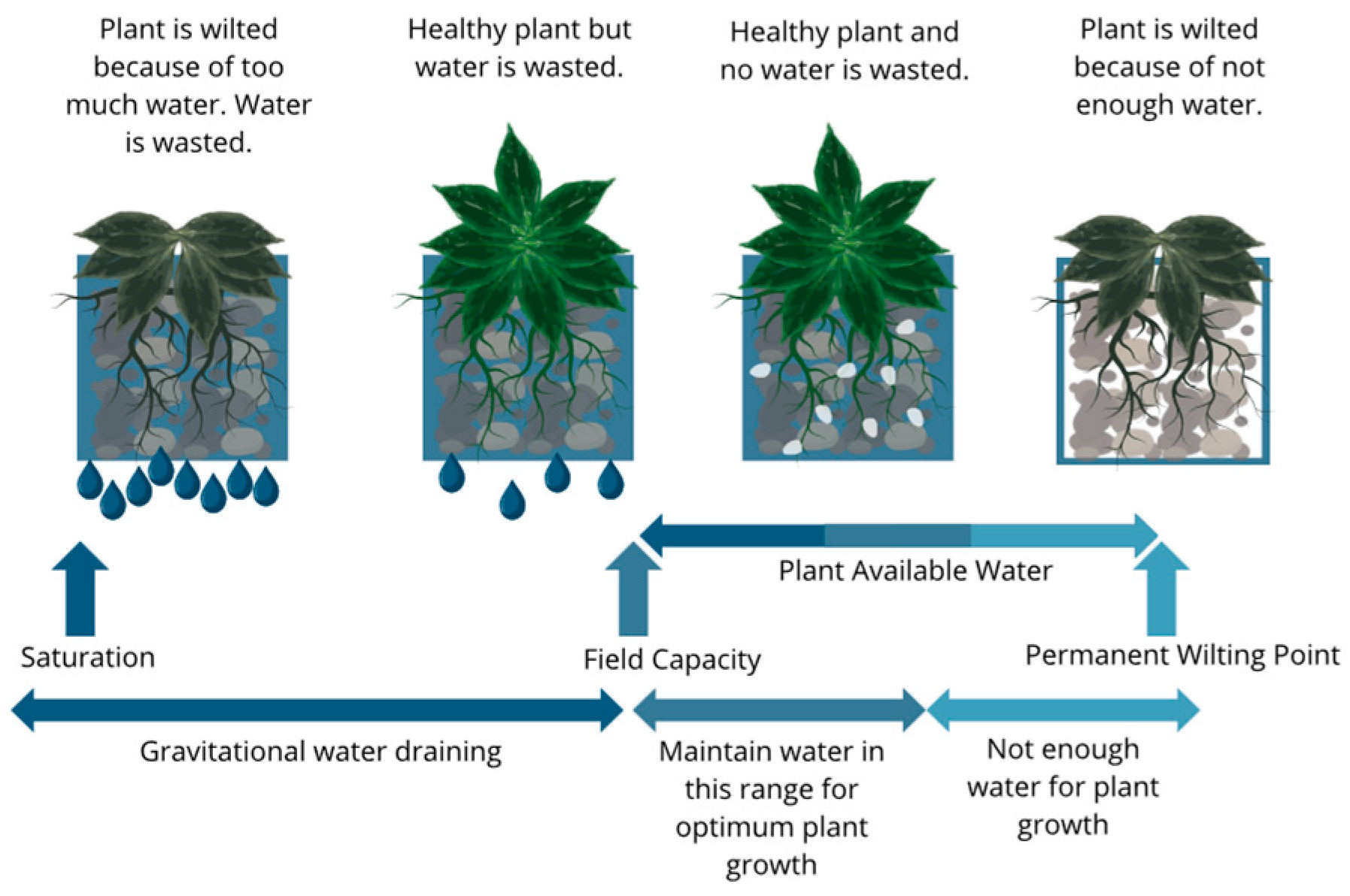
Efficient water management in agriculture is crucial for sustaining crop productivity, particularly in the face of climate change and increasing water scarcity. As can be seen in Figure 14, ASWMPs play a crucial role in maintaining optimal crop health by regulating soil moisture levels. This graph illustrates four key conditions: (i) over-saturation, where excess water causes plant stress and waste; (ii) field capacity, where plants remain healthy, but some water is lost; (iii) optimal moisture, which supports vigorous growth without waste; and (iv) drought conditions, leading to wilting and irreversible damage. Hence, maintaining soil moisture within the “plant available water” range is essential for maximizing crop productivity and minimizing the depletion of natural resources. In this way, developing mathematical and computational models for predicting ASWMPs plays a vital role in optimizing irrigation strategies. Therefore, the models herein developed can be used to integrate SSHC, FC, and PWP into intelligent irrigation systems that dynamically adjust water application rates based on real-time data. By leveraging ML techniques, these advanced irrigation solutions conserve water and enhance crop resilience to drought and other environmental stresses [50,106,107,108].
High hydraulic conductivity in sandy soils leads to rapid drainage, requiring frequent irrigation to prevent moisture loss [109,110]. Conversely, fine-grained soils with low hydraulic conductivity retain water longer but can lead to poor aeration and root suffocation if over-irrigated [111]. Thus, smart irrigation systems integrate hydraulic conductivity data to determine the optimal irrigation frequency and duration [112]. By incorporating FC data into irrigation management, intelligent systems can ensure soil moisture remains within the optimal range for plant growth. Automated irrigation controllers adjust watering cycles to maintain soil moisture near field capacity without exceeding it, thus avoiding unnecessary water wastage and preventing nutrient leaching [113]. This precision is particularly beneficial in mitigating the impacts of drought, as crops are consistently supplied with adequate moisture. Moreover, ML-driven irrigation technologies use soil moisture sensors to detect when soil moisture approaches the PWP and trigger irrigation before plant stress occurs. This proactive approach enhances crop resilience to drought conditions by maintaining a stable water supply even during periods of low rainfall [112].
Accordingly, smart irrigation systems optimize water application rates and irrigation schedules by integrating real-time readings of SSHC, FC, and PWP. These systems further enhance decision-making by leveraging ML-based models to forecast future water requirements based on historical data and climatic variables. Because of climate change, uneven distribution of precipitation, and constantly increasing annual average air temperature, integrating soil science with smart irrigation will be key to addressing global water challenges and ensuring food security [114,115,116].

5.4. Future Research Lines

Future research lines should focus on enhancing the accuracy and applicability of ASWMP estimation models by incorporating additional soil properties, particularly organic carbon content, which plays a crucial role in soil–water interactions and was not included in this study due to database limitations. Future efforts should also explore the role of biological factors, such as microbial activity and root-soil interactions, to develop more holistic and ecophysiologically relevant ASWMP models, ultimately improving precision irrigation strategies and sustainable soil management. Expanding datasets to include a wider range of soil types, climatic conditions, and management practices would also strengthen model generalizability.
On the other hand, developing real-time measurement techniques and integrating sensor-based monitoring systems could enable dynamic predictions of ASWMPs, improving adaptability to changing environmental conditions. Additionally, integrating advanced ML techniques with mechanistic soil–water models could enhance both predictive performance and interpretability, bridging the gap between data-driven insights and agronomic decision-making.

6. Conclusions

This study presents a comprehensive investigation into ASWMP prediction using both traditional mathematical models and advanced computational techniques. Through the analysis of 900 soil samples from the NaneSoil database, this research provides valuable insights into the relationships between the fundamental physical properties of soils and ASWMPs, as well as the effectiveness of different modelling approaches. Based on the results obtained, the following conclusions can be drawn:
  • The findings reveal strong correlations between the input variables (i.e., DBD, sand content, silt content, and clay content) and the ASWMPs (i.e., SSHC, FC, and PWP). In addition, mathematical models derived from these correlations demonstrate high accuracy in estimating ASWMPs, making them suitable for preliminary estimations in daily engineering practices.
  • DBD correlates significantly with SSHC, confirming that soil density influences its hydraulic conductivity. Meanwhile, clay content strongly correlates with SSHC, FC, and PWP, highlighting its importance in determining these ASWMPs. This underscores the importance of soil texture in water retention and movement.
  • This study also highlights the limitations of traditional mathematical models in capturing complex relationships, particularly when compared to advanced computational models such as DNNs. The introduction of a DNN-based model offers a promising approach for improving prediction accuracy and uncovering hidden relationships that may not be evident through traditional statistical methods.
  • The developed DNN-based model exhibits exactness between 91.4 and 99.7%, thereby exceeding the accuracy of the proposed statistical correlations (i.e., 71.7–96.4%).
Overall, this study enhances the understanding of soil–water interaction and provides practical tools for informed decision-making in agricultural management, particularly in the context of smart irrigation systems. By combining traditional mathematical models with advanced computational techniques and leveraging interpretability methods such as PDP and SHAP analyses, this research paves the way for more accurate and efficient ASWMP prediction, ultimately supporting sustainable agricultural practices and resource management strategies.

Author Contributions

Conceptualization, O.G.-B. and M.M.; methodology, O.G.-B. and M.M.; software, O.G.-B. and J.D.; validation, B.T. and J.D.; formal analysis, B.T. and O.G.-B.; investigation, O.G.-B., M.M. and J.D.; resources, J.D.; data curation, O.G.-B. and J.D.; writing—original draft preparation, O.G.-B.; writing—review and editing, B.T., M.M., J.D. and R.P.-M.; visualization, O.G.-B., J.D. and R.P.-M.; supervision, B.T. and J.D.; project administration, J.D. All authors have read and agreed to the published version of the manuscript.

Funding

This research received no external funding.

Data Availability Statement

The original contributions presented in this study are included in the article. The developed DNN-based model has been hosted in a public GitHub 3.16.1 repository, which can be accessed through the following link: https://github.com/OswaldoGCUC/DNN-ASWMPs (accessed on 6 March 2025). Further inquiries can be directed to the corresponding authors.

Conflicts of Interest

The authors declare no conflicts of interest.

Abbreviations

The following abbreviations are used in this manuscript:
ANNArtificial Neural Network
ASWMPsAgricultural Soil–Water Management Properties
DBDDry Bulk Density
DNNDeep Neural Network
EDiEstimated Data Point
EDRExponential Decay Rate
FCField Capacity
MAEMean Absolute Error
MAPEMean Absolute Percentage Error
MSEMean Squared Error
MSLEMean Squared Logarithm Error
MLMachine Learning
ODiOriginal/Experimental Data Point
PDPPartial Dependence Plot
PWPPermanent Wilting Point
R2Coefficient of Determination
RAMRandom-Access Memory
SHAPSHapley Additive exPlanations
SSHCSoil Saturated Hydraulic Conductivity
tanhTangent Hyperbolic

References

  1. USDA Practice Code 449: Irrigation Water Management Plan-Small Farms and Gardens; Natural Resources Conservation Service, United States Department of Agriculture: Washington, DC, USA, 2023; pp. 1–8.
  2. Flores-Saavedra, M.; Plazas, M.; Vilanova, S.; Prohens, J.; Gramazio, P. Induction of Water Stress in Major Solanum Crops: A Review on Methodologies and Their Application for Identifying Drought Tolerant Materials. Sci. Hortic. 2023, 318, 112105. [Google Scholar] [CrossRef]
  3. Ihuoma, S.O.; Madramootoo, C.A. Recent Advances in Crop Water Stress Detection. Comput. Electron. Agric. 2017, 141, 267–275. [Google Scholar] [CrossRef]
  4. Silber-Coats, N.; Elias, E.; Fernald, K.; Gagliardi, M. Evaluating Alternative Crops as a Solution to Water Stress in the U.S. Southwest. Agric. Water Manag. 2025, 312, 109439. [Google Scholar] [CrossRef]
  5. Katsoulas, N.; Elvanidi, A.; Ferentinos, K.P.; Kacira, M.; Bartzanas, T.; Kittas, C. Crop Reflectance Monitoring as a Tool for Water Stress Detection in Greenhouses: A Review. Biosyst. Eng. 2016, 151, 374–398. [Google Scholar] [CrossRef]
  6. Zhou, Z.; Majeed, Y.; Diverres Naranjo, G.; Gambacorta, E.M.T. Assessment for Crop Water Stress with Infrared Thermal Imagery in Precision Agriculture: A Review and Future Prospects for Deep Learning Applications. Comput. Electron. Agric. 2021, 182, 106019. [Google Scholar] [CrossRef]
  7. Nasta, P.; Szabó, B.; Romano, N. Evaluation of Pedotransfer Functions for Predicting Soil Hydraulic Properties: A Voyage from Regional to Field Scales across Europe. J. Hydrol. Reg. Stud. 2021, 37, 100903. [Google Scholar] [CrossRef]
  8. Zhang, Y.; Weihermüller, L.; Toth, B.; Noman, M.; Vereecken, H. Analyzing Dual Porosity in Soil Hydraulic Properties Using Soil Databases for Pedotransfer Function Development. Vadose Zone J. 2022, 21, e20227. [Google Scholar] [CrossRef]
  9. Kumari, A.; Singh, D.K.; Sarangi, A.; Hasan, M.; Sehgal, V.K. Optimizing Wheat Supplementary Irrigation: Integrating Soil Stress and Crop Water Stress Index for Smart Scheduling. Agric. Water Manag. 2024, 305, 109104. [Google Scholar] [CrossRef]
  10. Pereira da Silva, A.J.; Rodrigues Pinheiro, E.A.; van Lier, Q. de J. Determination of Soil Hydraulic Properties and Its Implications for Mechanistic Simulations and Irrigation Management. Irrig. Sci. 2020, 38, 223–234. [Google Scholar] [CrossRef]
  11. Arbat, G.; Masseroni, D. The Use and Management of Agricultural Irrigation Systems and Technologies. Agriculture 2024, 14, 236. [Google Scholar] [CrossRef]
  12. Kirkham, M.B. Chapter 8: Field Capacity, Wilting Point, Available Water, and the Non-Limiting Water Range. In Principles of Soil and Plant Water Relations; Dana Dreibelbi: New York, NY, USA, 2005; pp. 101–115. [Google Scholar]
  13. Loiskand, W.; Kammerer, G. Soil Water Management. In Encyclopedia of Agrophysics; Springer: Dordrecht, The Netherlands, 2014; pp. 802–805. [Google Scholar]
  14. Altchenko, Y.; Villholth, K.G. Mapping Irrigation Potential from Renewable Groundwater in Africa—A Quantitative Hydrological Approach. Hydrol. Earth Syst. Sci. 2015, 19, 1055–1067. [Google Scholar] [CrossRef]
  15. Weir, P.; Dahlhaus, P. In Search of Pragmatic Soil Moisture Mapping at the Field Scale: A Review. Smart Agric. Technol. 2023, 6, 100330. [Google Scholar] [CrossRef]
  16. Dinamarca, D.I.; Galleguillos, M.; Seguel, O.; Faúndez Urbina, C. CLSoilMaps: A National Soil Gridded Database of Physical and Hydraulic Soil Properties for Chile. Sci. Data 2023, 10, 630. [Google Scholar] [CrossRef]
  17. Maynard, J.J.; Yeboah, E.; Owusu, S.; Buenemann, M.; Neff, J.C.; Herrick, J.E. Accuracy of Regional-to-Global Soil Maps for on-Farm Decision-Making: Are Soil Maps “Good Enough”? Soil 2023, 9, 277–300. [Google Scholar] [CrossRef]
  18. Nenkam, A.M.; Wadoux, A.M.J.C.; Minasny, B.; Silatsa, F.B.T.; Yemefack, M.; Ugbaje, S.U.; Akpa, S.; Van Zijl, G.; Bouasria, A.; Bouslihim, Y.; et al. Applications and Challenges of Digital Soil Mapping in Africa. Geoderma 2024, 449, 117007. [Google Scholar] [CrossRef]
  19. Marthews, T.R.; Quesada, C.A.; Galbraith, D.R.; Malhi, Y.; Mullins, C.E.; Hodnett, M.G.; Dharssi, I. High-Resolution Hydraulic Parameter Maps for Surface Soils in Tropical South America. Geosci. Model Dev. 2014, 7, 711–723. [Google Scholar] [CrossRef]
  20. Szabó, B.; Szatmári, G.; Takács, K.; Laborczi, A.; Makó, A.; Rajkai, K.; Pásztor, L. Mapping Soil Hydraulic Properties Using Random-Forest-Based Pedotransfer Functions and Geostatistics. Hydrol. Earth Syst. Sci. 2019, 23, 2615–2635. [Google Scholar] [CrossRef]
  21. Trejo-Alonso, J.; Fuentes, S.; Morales-Durán, N.; Chávez, C. Evaluation and Development of Pedotransfer Functions and Artificial Neural Networks to Saturation Moisture Content Estimation. Water 2023, 15, 220. [Google Scholar] [CrossRef]
  22. Keïta, A.; Zorom, M.; Faye, M.D.; Damba, D.D.; Konaté, Y.; Hayde, L.G.; Lidon, B. Achieving Real-World Saturated Hydraulic Conductivity: Practical and Theoretical Findings from Using an Exponential One-Phase Decay Model. Hydrology 2023, 10, 235. [Google Scholar] [CrossRef]
  23. Picciafuoco, T.; Morbidelli, R.; Flammini, A.; Saltalippi, C.; Corradini, C.; Strauss, P.; Blöschl, G. On the Estimation of Spatially Representative Plot Scale Saturated Hydraulic Conductivity in an Agricultural Setting. J. Hydrol. 2019, 570, 106–117. [Google Scholar] [CrossRef]
  24. Ghorbani, M.A.; Shamshirband, S.; Zare Haghi, D.; Azani, A.; Bonakdari, H.; Ebtehaj, I. Application of Firefly Algorithm-Based Support Vector Machines for Prediction of Field Capacity and Permanent Wilting Point. Soil Tillage Res. 2017, 172, 32–38. [Google Scholar] [CrossRef]
  25. Chen, S.; Huo, Z.; Xu, X.; Huang, G. A Conceptual Agricultural Water Productivity Model Considering under Field Capacity Soil Water Redistribution Applicable for Arid and Semi-Arid Areas with Deep Groundwater. Agric. Water Manag. 2019, 213, 309–323. [Google Scholar] [CrossRef]
  26. de Freitas, E.M.; Vital, T.N.B.; Guimarães, G.F.C.; da Silveira, F.A.; Gomes, C.N.; da Cunha, F.F. Determination of the Permanent Wilting Point of Physalis peruviana L. Horticulturae 2023, 9, 873. [Google Scholar] [CrossRef]
  27. Chagas Torres, L.; Keller, T.; Paiva de Lima, R.; Antônio Tormena, C.; Veras de Lima, H.; Giarola, N.F.B. Impacts of Soil Type and Crop Species on Permanent Wilting of Plants. Geoderma 2021, 384, 114798. [Google Scholar] [CrossRef]
  28. Zhang, J.; Guan, K.; Peng, B.; Jiang, C.; Zhou, W.; Yang, Y.; Pan, M.; Franz, T.E.; Heeren, D.M.; Rudnick, D.R.; et al. Challenges and Opportunities in Precision Irrigation Decision-Support Systems for Center Pivots. Environ. Res. Lett. 2021, 16, 053003. [Google Scholar] [CrossRef]
  29. Goyal, A.; Flammini, A.; Morbidelli, R.; Corradini, C.; Govindaraju, R.S. Impact of Observation Thresholds in the Assessment of Field-Scale Soil Saturated Hydraulic Conductivity. J. Hydrol. 2023, 626, 130310. [Google Scholar] [CrossRef]
  30. Yu, M.; Zhang, J.; Wei, L.; Wang, G.; Dong, W.; Liu, X. Impact of Soil Textures on Agricultural Drought Evolution and Field Capacity Estimation in Humid Regions. J. Hydrol. 2023, 626, 130257. [Google Scholar] [CrossRef]
  31. Wiecheteck, L.H.; Giarola, N.F.B.; de Lima, R.P.; Tormena, C.A.; Torres, L.C.; de Paula, A.L. Comparing the Classical Permanent Wilting Point Concept of Soil (−15,000 HPa) to Biological Wilting of Wheat and Barley Plants under Contrasting Soil Textures. Agric. Water Manag. 2020, 230, 105965. [Google Scholar] [CrossRef]
  32. Liu, L.; Ma, X. Prediction of Soil Field Capacity and Permanent Wilting Point Using Accessible Parameters by Machine Learning. AgriEngineering 2024, 6, 2592–2611. [Google Scholar] [CrossRef]
  33. McCauley, A.; Jones, C.; Jacobsen, J. Soil & Water Management Module I: Basic Soil Properties; Montana State University Extension Services, Montana State University: Bozeman, MT, USA, 2005. [Google Scholar]
  34. Morales-Durán, N.; Fuentes, S.; Chávez, C. A Soil Database from Queretaro, Mexico for Assessment of Crop and Irrigation Water Requirements. Sci. Data 2023, 10, 429. [Google Scholar] [CrossRef]
  35. Trejo-Alonso, J.; Fuentes, C.; Chávez, C.; Quevedo, A.; Gutierrez-Lopez, A.; González-Correa, B. Saturated Hydraulic Conductivity Estimation Using Artificial Neural Networks. Water 2021, 13, 705. [Google Scholar] [CrossRef]
  36. Trejo-Alonso, J.; Quevedo, A.; Fuentes, C.; Chávez, C. Evaluation and Development of Pedotransfer Functions for Predicting Saturated Hydraulic Conductivity for Mexican Soils. Agronomy 2020, 10, 1516. [Google Scholar] [CrossRef]
  37. Polo-Mendoza, R.; Martinez-Arguelles, G.; Peñabaena-Niebles, R.; Duque, J. Development of a Machine Learning (ML)-Based Computational Model to Estimate the Engineering Properties of Portland Cement Concrete (PCC). Arab. J. Sci. Eng. 2024, 49, 14351–14365. [Google Scholar] [CrossRef]
  38. Polo-Mendoza, R.; Martinez-Arguelles, G.; Peñabaena-Niebles, R. Environmental Optimization of Warm Mix Asphalt (WMA) Design with Recycled Concrete Aggregates (RCA) Inclusion through Artificial Intelligence (AI) Techniques. Results Eng. 2023, 17, 100984. [Google Scholar] [CrossRef]
  39. Navarro-Rodríguez, A.; Castro-Artola, O.A.; García-Guerrero, E.E.; Aguirre-Castro, O.A.; Tamayo-Pérez, U.J.; López-Mercado, C.A.; Inzunza-Gonzalez, E. Recent Advances in Early Earthquake Magnitude Estimation by Using Machine Learning Algorithms: A Systematic Review. Appl. Sci. 2025, 15, 3492. [Google Scholar] [CrossRef]
  40. Wang, T.; Zuo, Y.; Manda, T.; Hwarari, D.; Yang, L. Harnessing Artificial Intelligence, Machine Learning and Deep Learning for Sustainable Forestry Management and Conservation: Transformative Potential and Future Perspectives. Plants 2025, 14, 998. [Google Scholar] [CrossRef]
  41. Ahsan, M.M.; Mahmud, M.A.P.; Saha, P.K.; Gupta, K.D.; Siddique, Z. Effect of Data Scaling Methods on Machine Learning Algorithms and Model Performance. Technologies 2021, 9, 52. [Google Scholar] [CrossRef]
  42. Mukhamediev, R.I.; Popova, Y.; Kuchin, Y.; Zaitseva, E.; Kalimoldayev, A.; Symagulov, A.; Levashenko, V.; Abdoldina, F.; Gopejenko, V.; Yakunin, K.; et al. Review of Artificial Intelligence and Machine Learning Technologies: Classification, Restrictions, Opportunities and Challenges. Mathematics 2022, 10, 2552. [Google Scholar] [CrossRef]
  43. Gombolay, G.Y.; Gopalan, N.; Bernasconi, A.; Nabbout, R.; Megerian, J.T.; Siegel, B.; Hallman-Cooper, J.; Bhalla, S.; Gombolay, M.C. Review of Machine Learning and Artificial Intelligence (ML/AI) for the Pediatric Neurologist. Pediatr. Neurol. 2023, 141, 42–51. [Google Scholar] [CrossRef]
  44. Tapeh, A.T.G.; Naser, M.Z. Artificial Intelligence, Machine Learning, and Deep Learning in Structural Engineering: A Scientometrics Review of Trends and Best Practices. Arch. Comput. Methods Eng. 2023, 30, 115–159. [Google Scholar] [CrossRef]
  45. Kujawa, S.; Niedbala, G. Artificial Neural Networks in Agriculture. Agriculture 2021, 11, 497. [Google Scholar] [CrossRef]
  46. Castillo-Girones, S.; Munera, S.; Martínez-Sober, M.; Blasco, J.; Cubero, S.; Gómez-Sanchis, J. Artificial Neural Networks in Agriculture, the Core of Artificial Intelligence: What, When, and Why. Comput. Electron. Agric. 2025, 230, 109938. [Google Scholar] [CrossRef]
  47. Attri, I.; Awasthi, L.K.; Sharma, T.P.; Rathee, P. A Review of Deep Learning Techniques Used in Agriculture. Ecol. Inform. 2023, 77, 102217. [Google Scholar] [CrossRef]
  48. Susanti, R.; Nofendra, R.; Zaini; Suhaimi, M.; Rusydi, M. The Use of Artificial Neural Networks in Agricultural Plants. Andalas J. Electr. Electron. Eng. Technol. 2022, 2, 62–68. [Google Scholar] [CrossRef]
  49. Basir, M.S.; Chowdhury, M.; Islam, M.N.; Ashik-E-Rabbani, M. Artificial Neural Network Model in Predicting Yield of Mechanically Transplanted Rice from Transplanting Parameters in Bangladesh. J. Agric. Food Res. 2021, 5, 100186. [Google Scholar] [CrossRef]
  50. Phogat, M.; Kumar, A.; Nandal, D.; Shokhanda, J. A Novel Automating Irrigation Techniques Based on Artificial Neural Network and Fuzzy Logic. J. Phys. Conf. Ser. 2021, 1950, 012088. [Google Scholar] [CrossRef]
  51. Polo-Mendoza, R.; Martinez-Arguelles, G.; Peñabaena-Niebles, R.; Covilla-Valera, E. Neural Networks Implementation for the Environmental Optimisation of the Recycled Concrete Aggregate Inclusion in Warm Mix Asphalt. Road Mater. Pavement Des. 2024, 25, 941–966. [Google Scholar] [CrossRef]
  52. de Amorim, L.B.V.; Cavalcanti, G.D.C.; Cruz, R.M.O. The Choice of Scaling Technique Matters for Classification Performance. Appl. Soft Comput. 2023, 133, 109924. [Google Scholar] [CrossRef]
  53. Sharma, V. A Study on Data Scaling Methods for Machine Learning. Int. J. Glob. Acad. Sci. Res. 2022, 1, 31–42. [Google Scholar] [CrossRef]
  54. Herwanto, H.W.; Handayani, A.N.; Wibawa, A.P.; Chandrika, K.L.; Arai, K. Comparison of Min-Max, Z-Score and Decimal Scaling Normalization for Zoning Feature Extraction on Javanese Character Recognition. In Proceedings of the 7th International Conference on Electrical, Electronics and Information Engineering (ICEEIE), Malang, Indonesia, 2 October 2021; pp. 457–459. [Google Scholar]
  55. Sinsomboonthong, S. Performance Comparison of New Adjusted Min-Max with Decimal Scaling and Statistical Column Normalization Methods for Artificial Neural Network Classification. Int. J. Math. Math. Sci. 2022, 2022, 3584406. [Google Scholar] [CrossRef]
  56. Kim, Y.-S.; Kim, M.K.; Fu, N.; Liu, J.; Wang, J.; Srebric, J. Investigating the Impact of Data Normalization Methods on Predicting Electricity Consumption in a Building Using Different Artificial Neural Network Models. Sustain. Cities Soc. 2024, 118, 105570. [Google Scholar] [CrossRef]
  57. Shen, S.-L.; Zhang, N.; Zhou, A.; Yin, Z.-Y. Enhancement of Neural Networks with an Alternative Activation Function TanhLU. Expert Syst. Appl. 2022, 199, 117181. [Google Scholar] [CrossRef]
  58. Fathi, E.; Maleki Shoja, B. Chapter 9: Deep Neural Networks for Natural Language Processing. In Handbook of Statistics; Elsevier: Amsterdam, The Netherlands, 2018; Volume 38, pp. 229–316. [Google Scholar]
  59. Kandel, I.; Castelli, M.; Popovič, A. Comparative Study of First Order Optimizers for Image Classification Using Convolutional Neural Networks on Histopathology Images. J. Imaging 2020, 6, 92. [Google Scholar] [CrossRef] [PubMed]
  60. Hassan, E.; Shams, M.Y.; Hikal, N.A.; Elmougy, S. The Effect of Choosing Optimizer Algorithms to Improve Computer Vision Tasks: A Comparative Study. Multimed. Tools Appl. 2023, 82, 16591–16633. [Google Scholar] [CrossRef]
  61. Yi, D.; Ahn, J.; Ji, S. An Effective Optimization Method for Machine Learning Based on ADAM. Appl. Sci. 2020, 10, 1073. [Google Scholar] [CrossRef]
  62. Qamar, T.; Bawany, N.Z. Understanding the Black-Box: Towards Interpretable and Reliable Deep Learning Models. PeerJ Comput. Sci. 2023, 9, e1629. [Google Scholar] [CrossRef]
  63. Hassija, V.; Chamola, V.; Mahapatra, A.; Singal, A.; Goel, D.; Huang, K.; Scardapane, S.; Spinelli, I.; Mahmud, M.; Hussain, A. Interpreting Black-Box Models: A Review on Explainable Artificial Intelligence. Cognit. Comput. 2024, 16, 45–74. [Google Scholar] [CrossRef]
  64. Taye, M.M. Understanding of Machine Learning with Deep Learning: Architectures, Workflow, Applications and Future Directions. Computers 2023, 12, 91. [Google Scholar] [CrossRef]
  65. Maier, H.R.; Galelli, S.; Razavi, S.; Castelletti, A.; Rizzoli, A.; Athanasiadis, I.N.; Sanchez-Marre, M.; Acutis, M.; Wu, W.; Humphrey, G.B. Exploding the Myths: An Introduction to Artificial Neural Networks for Prediction and Forecasting. Environ. Model. Softw. 2023, 167, 105776. [Google Scholar] [CrossRef]
  66. van der Westhuizen, S.; Heuvelink, G.B.M.; Gardner-Lubbe, S.; Clarke, C.E. Biplots for Understanding Machine Learning Predictions in Digital Soil Mapping. Ecol. Inform. 2024, 84, 102892. [Google Scholar] [CrossRef]
  67. Tatar, A.; Zeinijahromi, A.; Haghighi, M. Explainable Artificial Intelligence in Modelling Hydrogen Gas Solubility in N-Alkanes. Sep. Purif. Technol. 2025, 362, 131741. [Google Scholar] [CrossRef]
  68. Heger, J.; Min, A.; Zagst, R. Analyzing Credit Spread Changes Using Explainable Artificial Intelligence. Int. Rev. Financ. Anal. 2024, 94, 103315. [Google Scholar] [CrossRef]
  69. Zhao, X.; Yang, H.; Yao, Y.; Qi, H.; Guo, M.; Su, Y. Factors Affecting Traffic Risks on Bridge Sections of Freeways Based on Partial Dependence Plots. Phys. A Stat. Mech. Its Appl. 2022, 598, 127343. [Google Scholar] [CrossRef]
  70. Johnson, P.M.; Barbour, W.; Camp, J.V.; Baroud, H. Using Machine Learning to Examine Freight Network Spatial Vulnerabilities to Disasters: A New Take on Partial Dependence Plots. Transp. Res. Interdiscip. Perspect. 2022, 14, 100617. [Google Scholar] [CrossRef]
  71. Liang, B.; Liu, H.; Cressey, E.L.; Xu, C.; Shi, L.; Wang, L.; Dai, J.; Wang, Z.; Wang, J. Uncertainty of Partial Dependence Relationship between Climate and Vegetation Growth Calculated by Machine Learning Models. Remote Sens. 2023, 15, 2920. [Google Scholar] [CrossRef]
  72. Alomari, Y.; Andó, M. SHAP-Based Insights for Aerospace PHM: Temporal Feature Importance, Dependencies, Robustness, and Interaction Analysis. Results Eng. 2024, 21, 101834. [Google Scholar] [CrossRef]
  73. Gunduz, H.I.; Torun, A.T.; Gezgin, C. Post-Fire Burned Area Detection Using Machine Learning and Burn Severity Classification with Spectral Indices in Izmir: A SHAP-Driven XAI Approach. Fire 2025, 8, 121. [Google Scholar] [CrossRef]
  74. Bilgilioglu, S.S.; Gezgin, C.; Iban, M.C.; Bilgilioglu, H.; Gunduz, H.I.; Arslan, S. Explainable Sinkhole Susceptibility Mapping Using Machine-Learning-Based SHAP: Quantifying and Comparing the Effects of Contributing Factors in Konya, Türkiye. Appl. Sci. 2025, 15, 3139. [Google Scholar] [CrossRef]
  75. Gong, Y.; Zhang, Q.; Ren, Y.; Liu, Z.; Abu Seman, M.T. Research on Fuzzy Control of Methanol Distillation Based on SHAP (SHapley Additive ExPlanations) Interpretability and Generative Artificial Intelligence. Sensors 2025, 25, 1308. [Google Scholar] [CrossRef]
  76. Zhao, Z.; Wang, M.; Wei, J.; Cen, X.; Du, S.; Wu, Z.; Liu, H.; Wang, W. Interpretable Machine Learning for Multi-Energy Supply Station Revenue Forecasting: A SHAP-Driven Framework to Accelerate Urban Carbon Neutrality. Energies 2025, 18, 1624. [Google Scholar] [CrossRef]
  77. Guo, Y.; Ma, F.; Li, P.; Guo, L.; Liu, Z.; Huo, C.; Shi, C.; Zhu, L.; Gu, M.; Na, R.; et al. Comprehensive SHAP Values and Single-Cell Sequencing Technology Reveal Key Cell Clusters in Bovine Skeletal Muscle. Int. J. Mol. Sci. 2025, 26, 2054. [Google Scholar] [CrossRef] [PubMed]
  78. Goldstein, D.; Aldrich, C.; Shao, Q.; O’Connor, L. A Field-Scale Framework for Assessing the Influence of Measure-While-Drilling Variables on Geotechnical Characterization Using a Boruta-SHAP Approach. Mining 2025, 5, 20. [Google Scholar] [CrossRef]
  79. Lincoln, T.M.; Schlier, B.; Strakeljahn, F.; Gaudiano, B.A.; So, S.H.; Kingston, J.; Morris, E.M.J.; Ellett, L. Taking a Machine Learning Approach to Optimize Prediction of Vaccine Hesitancy in High Income Countries. Sci. Rep. 2022, 12, 2055. [Google Scholar] [CrossRef] [PubMed]
  80. Choi, H.; Kang, H.J.; Ahn, I.; Gwon, H.; Kim, Y.; Seo, H.; Cho, H.N.; Han, J.Y.; Kim, M.; Kee, G.; et al. Machine Learning Models to Predict the Warfarin Discharge Dosage Using Clinical Information of Inpatients from South Korea. Sci. Rep. 2023, 13, 22461. [Google Scholar] [CrossRef]
  81. Ghimire, S.; Abdulla, S.; Joseph, L.P.; Prasad, S.; Murphy, A.; Devi, A.; Barua, P.D.; Deo, R.C.; Acharya, R.; Yaseen, Z.M. Explainable Artificial Intelligence-Machine Learning Models to Estimate Overall Scores in Tertiary Preparatory General Science Course. Comput. Educ. Artif. Intell. 2024, 7, 100331. [Google Scholar] [CrossRef]
  82. Schaub, N.J.; Hotaling, N. Assessing Efficiency in Artificial Neural Networks. Appl. Sci. 2023, 13, 10286. [Google Scholar] [CrossRef]
  83. Ying, H.; Song, M.; Tang, Y.; Xiao, S.; Xiao, Z. Enhancing Deep Neural Network Training Efficiency and Performance through Linear Prediction. Sci. Rep. 2024, 14, 15197. [Google Scholar] [CrossRef]
  84. Bielecki, J.; Śmiałek, M. Estimation of Execution Time for Computing Tasks. Clust. Comput. 2023, 26, 3943–3956. [Google Scholar] [CrossRef]
  85. Wess, M.; Ivanov, M.; Unger, C.; Nookala, A.; Wendt, A.; Jantsch, A. ANNETTE: Accurate Neural Network Execution Time Estimation With Stacked Models. IEEE Access 2021, 9, 3545–3556. [Google Scholar] [CrossRef]
  86. Chen, W.; Qi, Z.; Akhtar, Z.; Siddique, K. Resistive-RAM-Based In-Memory Computing for Neural Network: A Review. Electronics 2022, 11, 3667. [Google Scholar] [CrossRef]
  87. Kaur, R.; Asad, A.; Mohammadi, F. A Comprehensive Review of Processing-in-Memory Architectures for Deep Neural Networks. Computers 2024, 13, 174. [Google Scholar] [CrossRef]
  88. Zeng, Z.; Cui, L.; Qian, M.; Zhang, Z.; Wei, K. A Survey on Sliding Window Sketch for Network Measurement. Comput. Netw. 2023, 226, 109696. [Google Scholar] [CrossRef]
  89. Pratheeksha, P.; Pranav, B.M.; Nasreen, A. Memory Optimization Techniques in Neural Networks: A Review. Int. J. Eng. Adv. Technol. 2021, 10, 44–48. [Google Scholar] [CrossRef]
  90. Wieczorek, J.; Guerin, C.; McMahon, T. K-Fold Cross-Validation for Complex Sample Surveys. Stat 2022, 11, 1–10. [Google Scholar] [CrossRef]
  91. White, J.; Power, S.D. K-Fold Cross-Validation Can Significantly Over-Estimate True Classification Accuracy in Common EEG-Based Passive BCI Experimental Designs: An Empirical Investigation. Sensors 2023, 23, 6077. [Google Scholar] [CrossRef] [PubMed]
  92. Zhang, L.; Luo, Z.; Su, B.; Song, Z.; Deng, J.; Ji, X. Prediction of Explosion Hazard of Aluminum Powder Two-Phase Mixed System Using Random Forest Based on K-Fold Cross-Validation. J. Loss Prev. Process Ind. 2025, 94, 105574. [Google Scholar] [CrossRef]
  93. Ait tchakoucht, T.; Elkari, B.; Chaibi, Y.; Kousksou, T. Random Forest with Feature Selection and K-Fold Cross Validation for Predicting the Electrical and Thermal Efficiencies of Air Based Photovoltaic-Thermal Systems. Energy Rep. 2024, 12, 988–999. [Google Scholar] [CrossRef]
  94. Shebl, A.; Abriha, D.; Dawoud, M.; Ali Hussein Ali, M.; Csámer, Á. PRISMA vs. Landsat 9 in Lithological Mapping—A K-Fold Cross-Validation Implementation with Random Forest. Egypt. J. Remote Sens. Space Sci. 2024, 27, 577–596. [Google Scholar] [CrossRef]
  95. Ünalan, S.; Günay, O.; Akkurt, I.; Gunoglu, K.; Tekin, H.O. A Comparative Study on Breast Cancer Classification with Stratified Shuffle Split and K-Fold Cross Validation via Ensembled Machine Learning. J. Radiat. Res. Appl. Sci. 2024, 17, 101080. [Google Scholar] [CrossRef]
  96. H2O.ai H2O AutoML: Automatic Machine Learning. Available online: https://docs.h2o.ai/h2o/latest-stable/h2o-docs/automl.html (accessed on 22 March 2025).
  97. Matta, A.; Matos, L.M.; Pilastri, A.; Silva, J.M.; Bastos Gomes, M.; Cortez, P. Ahead of Time Prediction of Decorated Particleboard Production Disruptions and Defects Using Single and Multi-Target AutoML. Procedia Comput. Sci. 2024, 246, 2110–2119. [Google Scholar] [CrossRef]
  98. Papík, M.; Papíková, L. The Possibilities of Using AutoML in Bankruptcy Prediction: Case of Slovakia. Technol. Forecast. Soc. Change 2025, 215, 124098. [Google Scholar] [CrossRef]
  99. Bagnall, D.K.; Morgan, C.L.S.; Bean, G.M.; Liptzin, D.; Cappellazzi, S.B.; Cope, M.; Greub, K.L.H.; Rieke, E.L.; Norris, C.E.; Tracy, P.W.; et al. Selecting Soil Hydraulic Properties as Indicators of Soil Health: Measurement Response to Management and Site Characteristics. Soil Sci. Soc. Am. J. 2022, 86, 1206–1226. [Google Scholar] [CrossRef]
  100. Gülser, C.; Candemir, F. Using Soil Moisture Constants and Physical Properties to Predict Saturated Hydraulic Conductivity. Eurasian J. Soil Sci. 2014, 3, 77–81. [Google Scholar] [CrossRef]
  101. Tripathy, K.P.; Mishra, A.K. Deep Learning in Hydrology and Water Resources Disciplines: Concepts, Methods, Applications, and Research Directions. J. Hydrol. 2024, 628, 130458. [Google Scholar] [CrossRef]
  102. Kay, B.D. Chapter 13: Soil Structure and Organic Carbon: A Review. In Soil Processes and the Carbon Cycle; Taylor Francis Group: Abingdon, UK, 1998; pp. 1–29. [Google Scholar]
  103. Rawls, W.J.; Pachepsky, Y.A.; Ritchie, J.C.; Sobecki, T.M.; Bloodworth, H. Effect of Soil Organic Carbon on Soil Water Retention. Geoderma 2003, 116, 61–76. [Google Scholar] [CrossRef]
  104. Panagea, I.S.; Berti, A.; Čermak, P.; Diels, J.; Elsen, A.; Kusá, H.; Piccoli, I.; Poesen, J.; Stoate, C.; Tits, M.; et al. Soil Water Retention as Affected by Management Induced Changes of Soil Organic Carbon: Analysis of Long-Term Experiments in Europe. Land 2021, 10, 1362. [Google Scholar] [CrossRef]
  105. Bienes, R.; Marques, M.J.; Sastre, B.; García-Díaz, A.; Esparza, I.; Antón, O.; Navarrete, L.; Hernánz, J.L.; Sánchez-Girón, V.; Sánchez del Arco, M.J.; et al. Tracking Changes on Soil Structure and Organic Carbon Sequestration after 30 Years of Different Tillage and Management Practices. Agronomy 2021, 11, 291. [Google Scholar] [CrossRef]
  106. Younes, A.; Elassad, Z.E.A.; El Meslouhi, O.; Elassad, D.E.A.; Majid, E.-D.A. The Application of Machine Learning Techniques for Smart Irrigation Systems: A Systematic Literature Review. Smart Agric. Technol. 2024, 7, 100425. [Google Scholar] [CrossRef]
  107. Pathmudi, V.R.; Khatri, N.; Kumar, S.; Abdul-Qawy, A.S.H.; Vyas, A.K. A Systematic Review of IoT Technologies and Their Constituents for Smart and Sustainable Agriculture Applications. Sci. Afr. 2023, 19, e01577. [Google Scholar] [CrossRef]
  108. Del-Coco, M.; Leo, M.; Carcagnì, P. Machine Learning for Smart Irrigation in Agriculture: How Far along Are We? Information 2024, 15, 306. [Google Scholar] [CrossRef]
  109. Viana, J.L.; de Souza, J.L.M.; Auler, A.C.; de Oliveira, R.A.; Araújo, R.M.; Hoshide, A.K.; de Abreu, D.C.; da Silva, W.M. Water Dynamics and Hydraulic Functions in Sandy Soils: Limitations to Sugarcane Cultivation in Southern Brazil. Sustainability 2023, 15, 7456. [Google Scholar] [CrossRef]
  110. Indoria, A.K.; Sharma, K.L.; Reddy, K.S. Chaper 18: Hydraulic Properties of Soil under Warming Climate. In Climate Change and Soil Interactions; Elsevier: Amsterdam, The Netherlands, 2020; pp. 473–508. [Google Scholar]
  111. Awedat, A.M.; Zhu, Y.; Bennett, J.M.L.; Raine, S.R. The Impact of Clay Dispersion and Migration on Soil Hydraulic Conductivity and Pore Networks. Geoderma 2021, 404, 115297. [Google Scholar] [CrossRef]
  112. Ahmed, Z.; Gui, D.; Murtaza, G.; Yunfei, L.; Ali, S. An Overview of Smart Irrigation Management for Improving Water Productivity under Climate Change in Drylands. Agronomy 2023, 13, 2113. [Google Scholar] [CrossRef]
  113. Nam, S.; Kang, S.; Kim, J. Maintaining a Constant Soil Moisture Level Can Enhance the Growth and Phenolic Content of Sweet Basil Better than Fluctuating Irrigation. Agric. Water Manag. 2020, 238, 106203. [Google Scholar] [CrossRef]
  114. Bwambale, E.; Abagale, F.K.; Anornu, G.K. Smart Irrigation for Climate Change Adaptation and Improved Food Security. In Irrigation and Drainage-Recent Advances; Muhammad, S., Ahmad, F., Eds.; IntechOpen: London, UK, 2022; pp. 1–18. [Google Scholar]
  115. Li, M.; Zhou, S.; Shen, S.; Wang, J.; Yang, Y.; Wu, Y.; Chen, F.; Lei, Y. Climate-Smart Irrigation Strategy Can Mitigate Agricultural Water Consumption While Ensuring Food Security under a Changing Climate. Agric. Water Manag. 2024, 292, 108663. [Google Scholar] [CrossRef]
  116. Durmuş, Y.; Arslansoy, G.; Gürbüz, T.K. Impact of Smart Irrigation Systems and Water Management on Climate Change. BIO Web Conf. 2024, 85, 01057. [Google Scholar] [CrossRef]
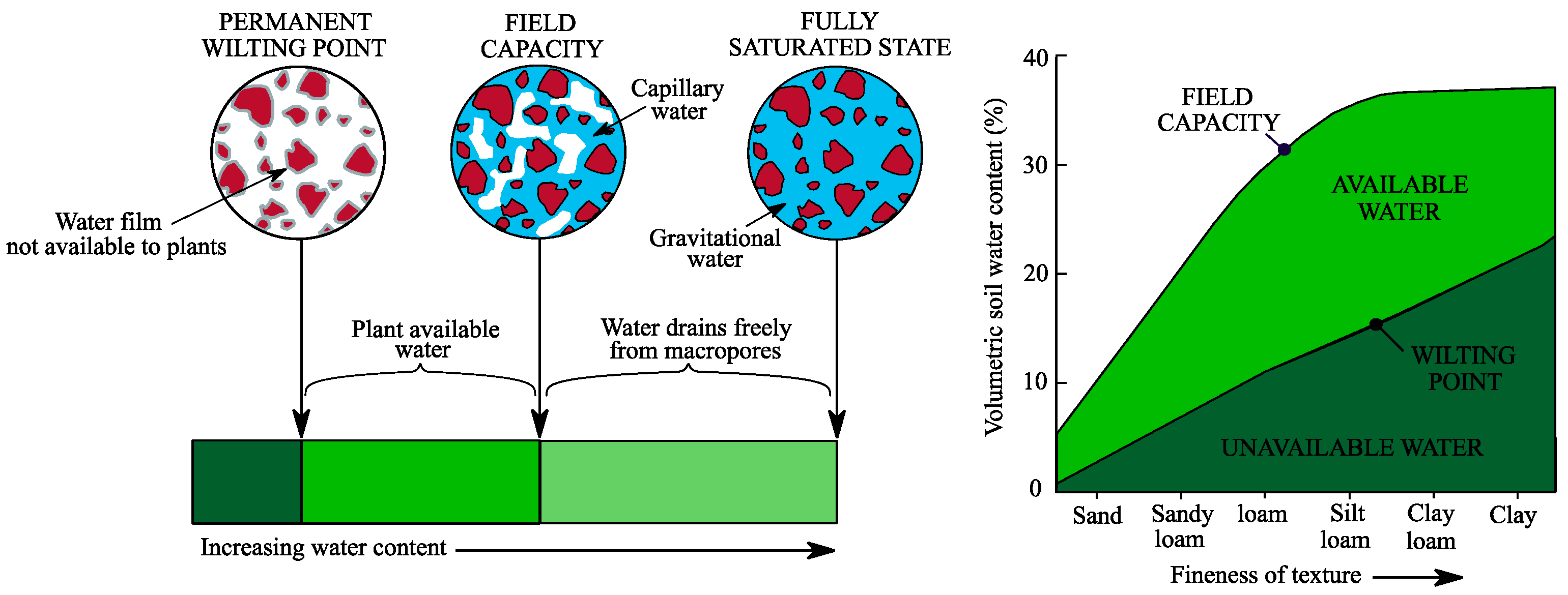
Figure 1. Relationship between fully saturated state, FC, and PWP. Adapted from [33].
Agronomy 15 00942 g001
Figure 2. Grain size distribution of the analyzed soil samples.
Agronomy 15 00942 g002
Figure 3. Scatterplot matrix of the addressed variables. Units: DBD—g/cm3; sand content—%/100; silt content—%/100; clay content—%/100; SSHC—cm/day; FC—cm3/cm3; PWP—cm3/cm3.
Agronomy 15 00942 g003
Figure 4. Heatmap of the addressed variables.
Agronomy 15 00942 g004
Figure 5. Graphic analysis of the proposed mathematical models.
Agronomy 15 00942 g005
Figure 6. Proposed DNN model.
Agronomy 15 00942 g006
Figure 7. Evolution of the loss function and MSLE over the epochs.
Agronomy 15 00942 g007
Figure 8. Comparison of measured and predicted values (1:1 lines).
Agronomy 15 00942 g008
Figure 9. PDP for the proposed DNN.
Agronomy 15 00942 g009
Figure 10. SHAP analysis for the proposed DNN.
Agronomy 15 00942 g010
Figure 11. Efficiency analysis on the proposed DNN model.
Agronomy 15 00942 g011
Figure 12. Results of the k-fold cross-validation on the loss function.
Agronomy 15 00942 g012
Figure 13. Results of the modelling with H2O AutoML.
Agronomy 15 00942 g013
Figure 14. Impact of ASWMPs on crop health. Adapted from [1].
Agronomy 15 00942 g014
Table 1. Variety of studied soil samples.
Soil TexturesCrops
TypeNo. of Samples (-)TypeNo. of Samples (-)
Clay30Maize (Zea mays L.)180
Clay loam64Alfalfa (Medicago sativa L.)135
Loam106Barley (Hordeum vulgare L.)135
Sandy clay10Oats (Avena sativa L.)135
Sandy clay loam140Sorghum (Sorghum vulgare Pers.)135
Sandy loam108Wheat (Triticum aestivum L.)90
Silt136Beans (Phaseolus vulgaris L.)45
Silt loam150Carrots (Daucus carota L.)45
Silty clay23
Silty clay loam133
Table 2. Parameters and statistical tests associated with Equation (5).
ParametersCoefficients95% Confidence IntervalStatistical Tests
EstimateStd. ErrorLower LimitUpper Limitt ValuePr (>|t|)F ValuePr (>F)
Intercept0.235120.043700.149340.320895.3809.53 × 10−8
ln (DBD+1)0.280340.032890.215790.344888.524<2 ×10−163344.793<2.2 ×10⁻¹⁶
ln (sand+1)−0.512240.02604−0.56334−0.46113−19.671<2 ×10−164604.163<2.2 ×10⁻¹⁶
ln (silt+1)−0.237350.03064−0.29749−0.17721−7.7462.57 ×10−141126.254<2.2 ×10⁻¹⁶
ln (clay+1)0.289130.031950.226420.351839.049<2 ×10−1681.893<2.2 ×10⁻¹⁶
Model information
Residual standard error: 0.01726 on 895 degrees of freedom. Multiple R2: 0.911, Adjusted R2: 0.9106.
F-statistic: 2289 on 4 and 895 degrees of freedom, p-value: <2.2 ×10⁻¹⁶.
Table 3. Statistical description of the original variables.
Variable
(Unit)
MinimumMaximumMeanMedianStandard
Deviation
KurtosisSkewness
Input
Variables
DBD (g/cm3)1.02001.62501.28551.28000.1127−0.58560.1847
sand (%/100)0.00070.77830.31140.28350.2021−1.28700.1695
silt (%/100)0.00800.92000.46910.45270.2346−0.53200.5889
clay (%/100)0.02120.59460.21950.21740.1205−0.29310.2973
Input
Variables
SSHC (cm/day)1.2000123.600034.154118.720034.0005−0.17701.1713
FC (cm3/cm3)0.17500.47500.30130.29500.05770.31220.6273
PWP (cm3/cm3)0.07000.35900.15110.13800.05513.38491.6833
Table 4. Statistical description of the scaled variables.
Variable
(Unit)
MinimumMaximumMeanMedianStandard
Deviation
KurtosisSkewness
Input
Variables
DBD (-)−1.00001.0000−0.1223−0.14050.3725−0.58560.1847
sand (-)−1.00001.0000−0.2009−0.27260.5198−1.28700.1695
silt (-)−1.00001.00000.0112−0.02480.5145−0.53200.5889
clay (-)−1.00001.0000−0.3083−0.31570.4203−0.29310.2973
Input
Variables
SSHC (-)−1.00001.0000−0.4615−0.71370.5556−0.17701.1713
FC (-)−1.00001.0000−0.1577−0.20000.38460.31220.6273
PWP (-)−1.00001.0000−0.4391−0.52940.38103.38491.6833
Table 5. Number of trainable parameters.
LayerNumber of Neurons Received (Nr)Number of Biases
(Nb)
Number of Neurons Contained (Nc)Number of Parameters
[(Nr + Nb) × Nc]
First hidden layer4180400
Second hidden layer801806480
Third hidden layer801806480
Fourth hidden layer801806480
Output layer8013243
Total number of trainable parameters20,083
Table 6. Implementation of the Adamax optimizer.
Working Principle. Adapted from [37,61].Adopted
Hyperparameter Values
PseudocodeLegend
t, m, u, w = 0, 0, 0, 0
for t = 1 to T do
   gt = ▽w × w
   m = β1 × m + (1 − β1) × gt
   u = max(β2 × u, abs(gt))
   lr = lr/(1 − β1^t)
   w = w − lr × m/(u + ε)
end for
t—iteration index
m—first moment vector
u—exponentially weighted infinity norm
w—convergence parameter (weight variable)
T—number of iterations to reach the convergence
gt—gradient
β1—EDR for the first moment estimates
β2—EDR for the exponentially weighted infinity norm
lr—learning rate
ε—small constant for numerical stability
   β1 = 0.9
   β2 = 0.999
   lr = 0.0007
   ε = 0.0000001
Table 7. Goodness-of-fit parameters associated with the proposed DNN at the final epoch.
Output VariableGoodness-of-Fit ParameterDataset
TrainingTestingValidation
SSHCMSE0.00110.00340.0020
MSLE0.18490.12280.1266
MAE0.01620.02520.0207
MAPE0.13770.14600.0453
R20.99660.98730.9923
FCMSE0.00330.00380.0031
MSLE0.00690.00540.0035
MAE0.02590.03420.0331
MAPE0.19270.17930.2495
R20.97820.97360.9743
PWPMSE0.01030.01070.0070
MSLE0.02440.01380.0137
MAE0.03410.05230.0426
MAPE0.19260.61120.9279
R20.93250.91360.9397
Disclaimer/Publisher’s Note: The statements, opinions and data contained in all publications are solely those of the individual author(s) and contributor(s) and not of MDPI and/or the editor(s). MDPI and/or the editor(s) disclaim responsibility for any injury to people or property resulting from any ideas, methods, instructions or products referred to in the content.