Pareto Optimization for Selecting Discriminating Test Locations in Plant Breeding

Abstract

Developing improved food crop cultivars requires time-consuming field trials, and the selection of experimental planting locations plays a key role. In early experiments, a plant breeder may prefer locations that have the best ability to discriminate the main genotype effects, that is, to screen the potential high performers from the average-to-poor cultivars. Traditionally, this discriminative ability of locations has focused on precision, but recent work suggests that some locations may be more sensitive to changes in the main genotype effect, having a higher relative discriminative value. We show that while both valuable, these are competing measures, meaning that no location maximizes both precision and the relative discriminative value, and there is a tradeoff that should be considered by breeders. We address this tradeoff by constructing a set of discriminating locations using Pareto optimization. We first identify a set of locations that cannot be improved along one measure without deteriorating the other and then expand this set by adding locations that are not significantly worse. Visualization facilitates evaluating the tradeoff and provides decision support when making choices about locations based on breeder preferences and status of the field experiments. The method is illustrated using publicly available barley data.

1. Introduction

The selection of test locations in multi-environmental trials (METs) is based on multiple considerations that are not always well aligned. For example, a recent study demonstrates the tradeoff between precision, repeatability, and representativeness [1]. This tradeoff is perhaps not surprising, as each of those measures is addressing very different objectives for ideal test locations. But even with a common general objective, such as choosing locations that allow for good discrimination of the main effect of cultivars, there may be a tradeoff between test locations based on how this general objective is quantified. This paper addresses two different ways for evaluating test locations in METs with respect to determining which locations are most discriminative, demonstrates that there is a tradeoff, and proposes a method for resolving the tradeoff. As this work focuses exclusively on the ability to discriminate main effects, it is primarily applicable to early-stage experiments, where many cultivars are screened to significantly reduce the set of experimental cultivars based on observations from a single planting season.

Evaluating locations for discriminative value has been a relatively active research topic, and much of this work has been focused on the locations in a specific trial, involving the environment (location and year) where the trial is conducted. Widely used methods for analyzing MET data that include an evaluation of the value of each environment in the trials are genotype and genotype-by-environment (GGE) biplots [2,3] and additive main effects and multiplicative interaction (AMMI) analysis [4], and the relative value of each has been the subject of significant debate [5,6]. However, these methods are intended to analyze MET data after they have been observed, but they are not necessarily intended to plan the trials, that is, to determine which test locations should be included in the trial before it is conducted. This is an important distinction from the work presented here. In this paper, we propose how to evaluate locations as good for evaluating only the main genotype effect of cultivars with the intent to help select locations for early-stage trials, that is, in the planning stage of a trial. Once data from those trials are observed, these observations can then, for example, be analyzed utilizing AMMI analysis [7,8].

The key contribution of this work thus focuses on determining the value of locations in a way that could be used to decide which locations should be included in a trial for the purpose of discriminating the main effect of cultivars. Other work has considered the value of locations across years and suggests that locations with low variance are preferable, as observing cultivars in low-variance locations improves precision and hence makes it easier to identify differences between cultivars. This is generally true, not just for plant breeding trials but in general, as it is desirable to improve precision for any experiment. Furthermore, it is known that such statistical precision is not sufficient, as the genotype-by-environment (G × E) interaction effects for many crops are so large that even if statistical precision is sufficient to correctly rank cultivars in one environment, this may not correlate well with the rank in other environments or the average over all environments. Thus, the plant breeding precision of a location appears to be often taken as a combination of statistical precision (low variance) and G × E effects that do not substantially change the rank of the cultivars versus the overall or average rank [1,9]. This is intuitive, since if the rank in a particular location is the same (or almost the same) as the overall rank, then all that is needed is to obtain sufficient statistical precision in this location to correctly rank the experimental cultivars. However, achieving such precision is very difficult in practice, as it would typically require more replications than is practically feasible. A recently proposed method reduces the need for such high precision by using a regression model to determine if some locations are inherently better at discriminating cultivars [10], that is, if part of the genotype-by-environment interactions are inherent to the locations in the sense that some locations are more sensitive to changes in the genetic main effects than others. For each location, their method estimates a sensitivity of that location to changes in the genetic main effect, which we will refer to as the relative discriminative value (RDV) of the location. If the RDV of a location is high, the differences in the genotype main effect are exaggerated and thus, less statistical precision is needed to discriminate between those effects.

We show that there is a tradeoff between the traditional measure of precision [9] and the RDV of a location and thus show that some high-variance locations may in fact be very useful for discriminating cultivars even if the precision is low. We suggest that this may be especially true for early-stage experiments, where a small amount of available data does not lend itself to estimating performance with high precision and the RDV is more important. On the other hand, locations with low RDVs will still be useful for discriminating cultivars if they have high precision, especially if sufficient data are available to obtain precise estimates. To formally address this tradeoff, we propose a new method based on Pareto optimality. Here, a set of locations corresponding to a Pareto frontier is identified, that is, a set of locations that is not dominated by any other location with respect to both the RDV and precision, which means that the locations with better RDVs and precision are already in the Pareto frontier set. We then expand this set to include locations that are not significantly worse than locations on the Pareto frontiers. Locations that are not included in the expanded set have both poor RDVs and precision and should not be considered as favorable locations for discriminating cultivars when planning trials.

The new Pareto optimization method is applied to a malt barley dataset that was the subject of a previously mentioned recent study for optimizing MET locations [1]. The results show that high-variance locations can either be some of the best locations or some of the worst locations, and the RDV explains which case applies for each location. Furthermore, although the ideal location that maximizes both precision and the RDV does not exist, many locations can be excluded as poor along both measures. The Pareto optimization approach provides a set of locations that are all useful for discriminating cultivars but have a tradeoff between precision and the RDV and may thus be preferable at different stages of plant breeding experiments depending on the amount of data available.

2. Materials and Methods

2.1. Relative Discriminating Value of Locations

The linear regression model described here was previously proposed to evaluate the usefulness of locations to discriminate between the main effects of two genotypes [10]. Let $y_{ijk}$ be the phenotypic response of the genotype $i$ in location $j$ and year $k$, which is modeled based on the main genotype effects $g_i$, the main environmental effects $h_{jk}$, and interactions between the genotype and environment (G × E). First estimates ${\widehat{g}}_i$ are obtained from some standard model [4,11,12]. Given this estimate, the sensitivity of each location to the main genetic effect, that is, the interaction slopes $b_j$, can be estimated using a linear model that accounts for the environmental main effects (E), the estimated genetic main effect (G), and the interaction between the location and main genetic effect (G × E):

$$y_{ijk}=\mu +h_{jk}+\left(1+b_j\right){\widehat{g}}_i+{ϵ}_{ijk},$$

(1)

The estimated values ${\widehat{b}}_l$ for model (1) indicate how sensitive a location $l$ is to changes in the main genetic effect and will be referred to here as the relative discriminative value (RDV), ${RDV\left(l\right)=\widehat{b}}_l$. It is important to note that this value is relative to a base location that must be selected for the regression model. Any location could be selected as base location, but in this paper, the base location will be selected so that there is an equal number of locations with positive and negative values (although some of those values may not be significantly different from zero).

We reiterate that the primary purpose of examining the RDV and the tradeoff with precision is for the purpose of screening out poor and average cultivars when there are still many experimental cultivars under consideration, and before those cultivars have been planted in a sufficient number of environments, we aim to estimate G × E effects and consider the suitability of cultivars for different environments.

2.2. Precision of Locations

The RDV described above is a measure of the discriminative value of a location, but a more traditional approach is a measure of precision, that is, to consider a location more discriminative if it has less variance. This is intuitive; if precision is sufficiently good, then all the cultivars can be easily discriminated, meaning we could correctly compare and rank them. The problem is that such precision is not easily achievable and when the noise, that is, the random variation in the observed phenotypic values not explained by genotype or environment, is very high, it may be better to sacrifice precision for biased estimates that exaggerate differences in main effects, namely a location with a high relative discriminative value (RDV).

This paper uses the following method for calculating precision [1]: the lack of precision is quantified using the variance $V=\left(V_R+V_{GE}\right)/e$, where $V_R$ is the residual variance, $V_{GE}$ is the variance of the G × E interactions, and $e$ is the number of environments. This is consistent with the intuitive idea that the ability to correctly rank cultivars based on one location depends on both the traditional statistical variance being low and the interaction effects in that specific location not substantially changing the rank from the overall rank. Precision is improved as this expression of variance is decreased, and we thus define the precision of each location as the negative logarithm of the variance, namely

$$Precision\left(l\right)=-{\mathrm{l}\mathrm{o}\mathrm{g}}_{2}V.$$

(2)

We calculate (2) using the R code that is provided in a previous study [1], which is based on the ASREML-R package, where the reader can find a more detailed description.

The key contributions of this paper are to show how the relative discriminative value (RDV) obtained from the regression model (1) and precision obtained from Equation (2) provide complementary useful measures of discriminative locations, and we propose a new method based on Pareto optimization that incorporates both precision and the RDV to identify a set of the most discriminative locations.

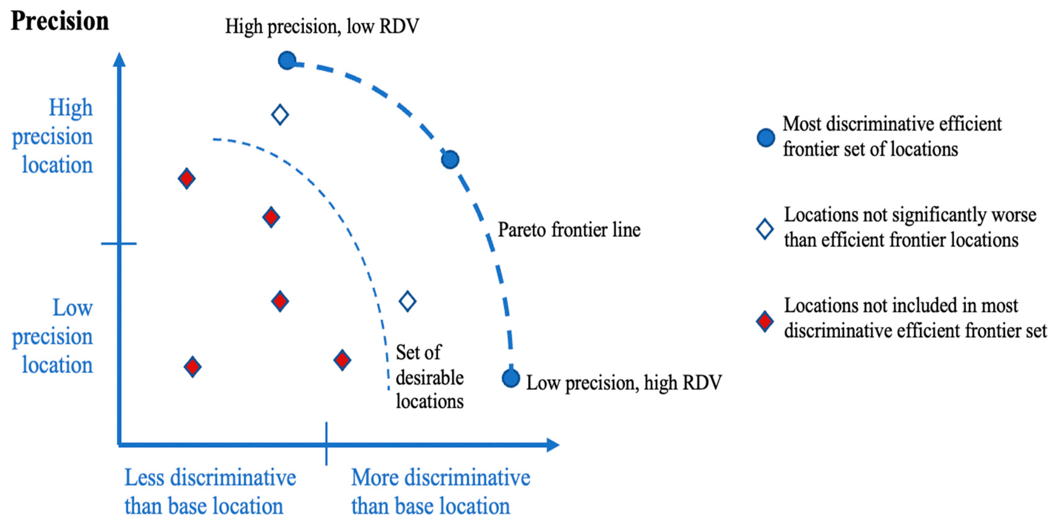
2.3. Pareto Optimization of Precision and RDV

As noted above, this paper combines the precision and RDVs of locations and uses this combination to eliminate poor locations and choose good locations. As noted above, we will show that there is a tradeoff between the RDV and precision, in that as precision increases, the RDV may decrease and vice versa. This paper addresses this tradeoff by considering the two simultaneously. Locations that are poor according to both measures may simply be considered non-discriminative, but for those locations that perform well according to at least one measure, the tradeoff must be addressed by evaluating both measures.

Specifically, to address this mathematically, we propose to start by identifying what may be termed the Pareto frontier for locations. Pareto optimization has been widely applied to solve problems with multiple objectives [13,14], including in other agricultural applications [15]. We first define the set $D\left(l\right)$ of locations that dominate location $l\in L$ on both measures, that is,

$$D\left(l\right)=\left\{l^{\prime }\in L:RDV\left(l^{\prime }\right)>RDV\left(l\right),Precision\left(l^{\prime }\right)>Precision\left(l\right),l^{\prime }\ne l\right\}.$$

Then, the Pareto frontier locations are defined as

$$L_{PF}=\{l\in L:D(l)=\mathrm{\varnothing }\},$$

(3)

where locations for which the set $D\left(l\right)$ are empty. Intuitively, this equation states that a location that has a better RDV and better precision than the locations on the Pareto frontier should be added to the Pareto frontier set until no location outside of the Pareto frontier set has a better RDV and precision. The set of Pareto frontier locations $L_{PF}$ are locations that are desirable from the perspective of discriminating main genotype effects, but since it is defined based on statistical estimates of both the precision and RDV, other locations may not be significantly worse and should hence also be included in a set of desirable locations. We thus define a set of desirable locations as follows: by changing the base location in the regression model (1) to each of the locations in $L_{PF}$ one at a time, we can determine a p value $p\left(l\right)$ for each of the locations not in $L_{PF}$ that indicates, according to the regression model, whether its RDV is significantly worse than the RDV of the location already in the Pareto frontier. We then expand the set $L_{PF}$ to include all locations that have either high precision or high RDVs relative to the locations in $L_{PF}$ and for which the RDV is not significantly worse than the location in $L_{PF}$ that has the most similar precision. We refer to this new set as $L_{DL}$. Thus, $L_{PF}$ are the Pareto frontier locations and the $L_{DL}$ are the desirable locations which are obtained by adding locations to the set $L_{PF}$.

The procedure described above for expanding the set $L_{PF}$ to a set $L_{DL}$ of desirable locations is formally described in the following steps:

Procedure for Constructing Set of Desirable Locations

Step 0. Start with just the locations in the Pareto frontier, that is, let $L_{DL}=L_{PF}$. Calculate the range of precision and RDVs in the Pareto frontier:

$$R_{RDV}=\underset{l\in L_{\mathit{PF}}}{\max }RDV\left(l\right)-\underset{l\in L_{\mathit{PF}}}{\min }RDV\left(l\right),$$

$$R_{Prec}=\underset{l\in L_{\mathit{PF}}}{\max }Precision\left(l\right)-\underset{l\in L_{\mathit{PF}}}{\min }Precision\left(l\right).$$

For each $l\in L\backslash L_{PF}$, repeat the following:

Step 1. Identify the location in $L_{PF}$ with the most similar precision:

$$l^0=\underset{l^{\prime }\in L_{\mathit{PF}}}{\mathrm{argmax}}\left|Precision\left(l\right)-Precision\left(l^{\prime }\right)\right|$$

Using l as base location in the regression model (1), determine a p value $p^{l^0}$ for $l^0$, indicating if this location l is significantly worse than $l^0$ with respect to the RDV, that is, determine if the RDV coefficients of these two locations are significantly different.

Step 2. If $RDV\left(l\right)>{\beta }_1{R}_{RDV}$ or $Precision\left(l\right)>{\beta }_2{R}_{Prec}$, and $p^{l^0}>\alpha$, add location l to the set of desirable locations, that is,

$$L_{DL}=L_{DL}\cup \left\{l\right\}.$$

Note that ${\beta }_1$ and ${\beta }_2$ are the primary parameters that determine how many locations are added. If ${\beta }_1={\beta }_2=1$, then no locations will be added and $L_{DL}=L_{PF}$. If ${\beta }_1={0 \mathrm{or} \beta }_2=0$, then every location will be added and $L_{DL}=L$. We recommend ${\beta }_1={\beta }_2={\displaystyle \frac{1}{2}}$ as the default, which simply states that to be added, a location $l\in L\backslash L_{PF}$ must have either better-than-average RDVs or precision compared to the $L_{PF}$ locations, but these parameter values could be decreased if a larger set of locations is desired or increased to obtain a more exclusive set of highly discriminative locations.

The sets $L_{PF}$ and $L_{DL}$ illustrated in Figure 1 show some hypothetical locations with known precision and RDVs. As mentioned before, an ideal location is a location with a high RDV and low variance, but typically, there is a tradeoff between the RDV and precision, which motivates using Pareto optimization to choose good locations. Here, three locations are not dominated by any other location on both precision and RDVs and hence form the Pareto frontier $L_{PF}$. A further two locations have either above average precision or an above average RDV compared to the Pareto frontier locations, as well as having an insignificantly worse RDV compared to the Pareto frontier location that has the most similar precision. Those two locations are hence added to the set of desirable locations, resulting in five locations in the set $L_{DL}$.

2.4. Data

The data used in this paper are obtained from a previously reported barley study [1], and we refer the reader to that paper for a complete description. These data consist of two regional barley trials, namely the Mississippi Valley Nursery (MVN), which includes the upper Mississippi River valley and Red River valley regions of the United States and Canada, and the Western Regional Nursery (WRN), which covers the western Great Plains and northern Intermountain West regions. These regions are representative of two sets of climates practices, rainfed and irrigated. In this dataset, the trials that are in the MVN region were entirely rainfed, while the trials in the WRN region were irrigated.

The phenotypic data in this dataset cover 426 location-year environments from 46 unique locations across 25 years from 1995 to 2019. This dataset contains 722 unique genotypes. As this study seeks to understand locations, there should be multiple years observed from each location, and our experience indicates that each location should be observed for at least three years. Hence, only frequently planted locations, namely those that have been tested for at least three years, are used. The number of unique frequent locations, their names for each nursery region for both the selected traits (grain yield and grain protein), and the base location used for calculations in this study can be seen in

Table 1. Two barley nursery regions and corresponding locations.

Nursery	Number of Locations			Name of the Locations
	Total	Grain Protein	Grain Yield
Mississippi Valley Nursery (MVN)	13	7	12	Aberdeen, Ames, Bottineau. Brandon, Carrington, Crookston, Fargo, Hamiota, Madison, Morris, Osnabrock, Saskatoon, Sidney
Western Regional Nursery (WRN)	24	5	12	Aberdeen, Bozeman, Conrad, Fairfield, Fargo, Hettinger, Idaho Falls, Klamath Falls, Langdon, Logan, Manhattan, McVille, Minot, Moscow, Moses Lake, Potlatch, Powell, Pullman, Saskatoon, Soda Springs, Sterling, Tetonia, Tulelake, Williston

.

We consider two phenotypes, grain protein and grain yield. Each of those can be argued as being of key importance to growers. For the MVN, there are 7 and 12 locations with sufficient observations for these two phenotypes, respectively, and for the WRN, there are 5 and 12 locations, respectively (see Table 1). As there is no overlap in genotypes, this study analyzed the WRN and MVN data separately.

3. Results

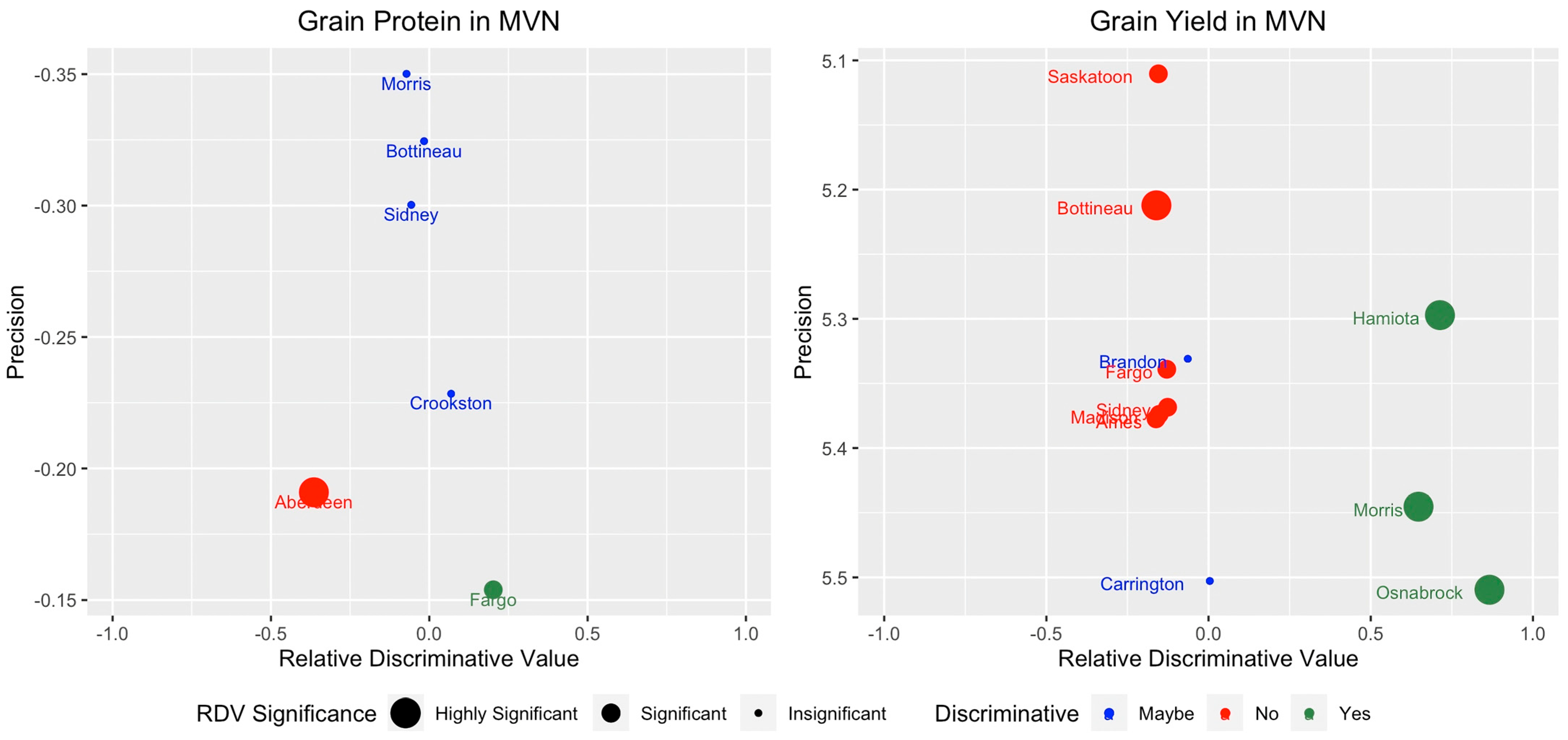
3.1. RDV and Precision Tradeoff for Discriminating Locations

The key premise of this paper is that we expect there to be a tradeoff between the RDV and precision for locations. In this section, we report the RDV and precision results for each planting location in the barley data. The numerical results, namely the precision and RDVs for every location considered, are reported in the Appendix A (see

Table A1. Full regression results for grain protein in the MVN region.

Locations	B Value (Estimate)	Standard Error	t-Value	p-Value
Aberdeen	−0.364	0.079	−4.563	$5.280 \times$ 10−6
Bottineau	−0.016	0.093	−0.174	$8.616 \times$ 10−1
Crookston	0.069	0.082	0.837	$4.024 \times$ 10−1
Fargo	0.202	0.087	2.311	$2.089 \times$ 10−2
Morris	−0.071	0.084	−0.847	$3.969 \times$ 10−1
Sidney	−0.056	0.090	−0.626	$5.311 \times$ 10−1

,

Table A2. Full regression results for grain yield in the MVN region.

Locations	B Value (Estimate)	Standard Error	t-Value	p-Value
Ames	−0.161	0.075	−2.154	$3.122 \times$ 10−2
Bottineau	−0.160	0.059	−2.711	$6.720 \times$ 10−3
Brandon	−0.064	0.070	−0.903	$3.663 \times$ 10−1
Carrington	0.003	0.058	0.065	$9.479 \times$ 10−1
Fargo	−0.128	0.059	−2.181	$2.921 \times$ 10−2
Hamiota	0.713	0.132	5.388	$7.472 \times$ 10−8
Madison	−0.152	0.059	−2.553	$1.068 \times$ 10−2
Morris	0.647	0.090	7.162	$9.250 \times$ 10−13
Osnabrock	0.866	0.094	9.157	$8.021 \times$ 10−20
Saskatoon	−0.154	0.068	−2.250	$2.444 \times$ 10−2
Sidney	−0.126	0.059	−2.110	$3.484 \times$ 10−2
Conrad	−0.194	0.088	−2.189	$2.869 \times$ 10−2
Fairfield	0.085	0.066	1.291	$1.967 \times$ 10−1
IdahoFalls	−0.298	0.061	−4.813	$1.615 \times$ 10−6
Pullman	0.034	0.077	−0.443	$6.574 \times$ 10−1

,

Table A3. Full regression results for grain yield in the WRN region.

Locations	B Value (Estimate)	Standard Error	t-Value	p-Value
Aberdeen	0.271	0.071	3.810	$1.394 \times$ 10−4
Conrad	−0.176	0.077	−2.264	$2.357 \times$ 10−2
Fairfield	0.157	0.072	2.180	$2.925 \times$ 10−2
Fargo	−0.237	0.067	−3.492	$4.806 \times$ 10−4
Hettinger	0.060	0.072	0.835	$4.035 \times$ 10−1
IdahoFalls	0.152	0.071	2.140	$3.236 \times$ 10−2
KlamathFalls	−0.110	0.078	−1.402	$1.607 \times$ 10−1
Langdon	−0.270	0.080	−3.364	$7.717 \times$ 10−4
Logan	0.247	0.072	3.423	$6.212 \times$ 10−4
Manhattan	0.790	0.204	3.860	$1.141 \times$ 10−4
McVille	0.617	0.116	5.299	$1.194 \times$ 10−7
Moscow	0.653	0.249	2.622	$8.753 \times$ 10−3
Potlatch	−0.267	0.082	−3.251	$1.150 \times$ 10−3
Powell	0.331	0.070	4.679	$2.928 \times$ 10−6
Saskatoon	−0.144	0.064	−2.234	$2.546 \times$ 10−2
Sterling	−0.194	0.077	−2.499	$1.245 \times$ 10−2
Tetonia	−0.145	0.072	−1.998	$4.565 \times$ 10−2
Tulelake	0.009	0.078	0.114	$9.085 \times$ 10−1
Williston	−0.025	0.071	−0.355	$7.221 \times$ 10−1

and

Table A4. Calculated precision of locations for both traits in each region.

Locations in MVN				Locations in WRN
Grain Protein	Precision	Grain Yield	Precision	Grain Protein	Precision	Yield	Precision
Aberdeen	−0.190	Ames	5.377	Conrad	−0.355	Aberdeen	5.656
Bottineau	−0.324	Bottineau	5.212	Fairfield	−0.133	Conrad	5.622
Crookston	−0.228	Brandon	5.330	IdahoFalls	−0.092	Fairfield	5.354
Fargo	−0.153	Carrington	5.502	Pullman	−0.149	Fargo	5.505
Morris	−0.350	Fargo	5.339			Hettinger	5.738
Sidney	−0.300	Hamiota	5.297			IdahoFalls	5.765
		Madison	5.373			KlamathFalls	5.386
		Morris	5.445			Langdon	5.796
		Osnabrock	5.509			Logan	5.539
		Saskatoon	5.110			Manhattan	5.511
		Sidney	5.368			McVille	5.562
						Moscow	5.736
						Potlatch	5.849
						Powell	5.442
						Saskatoon	5.316
						Sterling	5.309
						Tetonia	5.359
						Tulelake	5.863
						Williston	5.365

). Here, we report a visual summary of those results. Figure 2 and Figure 3 show graphs of the precision and RDVs for the locations in the MVN and WRN regions, respectively. Both grain protein and grain yield are considered as the phenotype. It should also be noted that all locations are contrasted against a neutral location (base location in the regression model), which has a slope $b=0$. The green points in the figures represent locations identified as desirable for discrimination, either on the Pareto frontier or added due to favorable precision or RDVs without significantly worse performance than frontier locations.

We consider the results from the MVN region first (Figure 2). For grain protein, we observe that Fargo is the location with the best RDV but is also the location with the worst precision (highest variability). For grain yield, Osnabrock is the location with the best RDV but has the worst precision. For grain yield, there are three locations with significantly high RDVs (Osnabrock, Morris, and Hamiota), All these locations have average or worse precision. Vice versa, the locations with the best precision (Morris for grain protein and Saskatoon for grain yield) have poor RDVs. Hamiota appears to be a location that strikes a balance between both, with a high RDV and average precision. In the WRN region (Figure 3), Moses Lake has the highest RDV for grain yield but has poor precision. McVille and Manhattan are similar to Hamiota in that they strike a balance with high RDVs and average precision. Such locations should certainly be considered in addition to the locations that have very good RDVs or very good precision. Grain protein in the WRN demonstrates the fact that a high-RDV location may not always exist. Here, there is just one location (Conrad) that should clearly be selected due to its superior precision. Based on these results, we observe that for these data, (a) the locations with the highest precision never have a significantly positive RDV, (b) the locations with large RDVs (either positive or negative) always have low precision and often the worst precision, and (c) some locations strike a balance between good precision and RDVs.

3.2. Pareto Optimality and Discriminative Locations

In this section, we report the sets $L_{DL}$ of desirable locations found in the barley data. The tradeoff between RDVs and precision observed for the locations in the barley data suggests that the Pareto optimality that was introduced in the methods above would be useful. Pareto optimality can be used to identify a set of locations with desirable discriminative properties, that is, locations that have either high precision, a large RDV, or strike a balance between the two measures.

This Pareto frontier for grain yields is shown in Figure 2 and Figure 3 to help identify the desirable set of locations. Grain yield is chosen rather than grain protein because there are not enough good versus poor locations for discriminating grain protein. This is especially true for the WRN region, where no location has a significant positive RDV for grain protein. Figure 4 shows the grain yield as in Figure 2 and Figure 3 with the addition of the proposed Pareto frontier and a shaded area indicating the desirable locations for discrimination. To determine how the set $L_{DL}$ is constructed from $L_{PF}$, we use the method described in Section 2.3 above with parameter ${\beta }_1={\beta }_2={\displaystyle \frac{1}{2}}$ and the pairwise p values of the locations that are reported in the Appendix A (see

Table A5. Calculated pairwise p value of good locations in the MVN region for grain yield. Significant (*) and highly significant (**) differences are indicated and used to determine how the Pareto frontier set of locations is expanded to all discriminative locations.

	Regression Model p Values
Base Location	Osnabrock	Morris	Hamiota	Saskatoon
Osnabrock	-	$6.165 \times$ 10−2 *	$3.145 \times$ 10−1	$1.200 \times$ 10−23 **
Morris	$6.165 \times$ 10−2 *	-	$6.582 \times$10−1	$2.248 \times$ 10−16 **
Hamiota	$3.145 \times$ 10−1	$6.582 \times$10−1	-	$2.773 \times$ 10−10 **

and

Table A6. Calculated pairwise p value of good locations in the WRN region for grain yield. Significant (*) and highly significant (**) differences are indicated and used to determine how the Pareto frontier set of locations is expanded to all discriminative locations.

	Regression Model p Value
Base Location	Williston	Sterling	Fargo	Saskatoon	Tetonia	McVille	Manhattan	Moses Lake	Langdon
MosesLake	2.031 $\times$ 10−11 **	1.264 $\times$ 10−14 **	1.100 $\times$ 10−16 **	1.181 $\times$ 10−14 **	6.115 $\times$ 10−14 **	7.131 $\times$ 10−2 *	5.827 $\times$ 10−1	-	3.565 $\times$ 10−16 **
Manhattan	6.878 $\times$ 10−5 **	2.041 $\times$ 10−6 **	4.650 $\times$ 10−7 **	4.023 $\times$ 10−6 **	5.263 $\times$ 10−6 **	4.411 $\times$ 10−1	-	5.827 $\times$ 10−1	3.562 $\times$ 10−7 **
McVille	3.691 $\times$ 10−8 **	1.921 $\times$ 10−11 **	1.011 $\times$ 10−13 **	1.521 $\times$ 10−11 **	9.591 $\times$ 10−11 **	-	4.411 $\times$ 10−1	7.131 $\times$ 10−2 *	4.593 $\times$ 10−13 **
Tetonia	9.944 $\times$ 10−2 *	5.427 $\times$ 10−1	1.926 $\times$ 10−1	9.830 $\times$ 10−1	-	9.591 $\times$ 10−11 **	5.263 $\times$ 10−6 **	6.115 $\times$ 10−14 **	1.298 $\times$ 10−1
Saskatoon	6.624 $\times$ 10−2 *	4.887 $\times$ 10−1	1.305 $\times$ 10−1	-	9.830 $\times$ 10−1	1.521 $\times$ 10−11 **	4.023 $\times$ 10−6 **	1.181 $\times$ 10−13 **	9.264 $\times$ 10−2 *
Fargo	1.876 $\times$ 10−3 **	5.684 $\times$ 10−1	-	1.305 $\times$ 10−1	1.926 $\times$ 10−1	1.011 $\times$ 10−13 **	4.650 $\times$ 10−7 **	1.100 $\times$ 10−16 **	6.684 $\times$ 10−1
Sterling	3.011 $\times$ 10−2 *	-	5.684 $\times$ 10−1	4.887 $\times$ 10−1	5.427 $\times$ 10−1	1.921 $\times$ 10−11 **	2.041 $\times$ 10−6 **	1.264 $\times$ 10−14 **	3.790 $\times$ 10−1
Langdon	2.354 $\times$ 10−3 **	3.790 $\times$ 10−1	6.684 $\times$ 10−1	9.264 $\times$ 10−2 *	1.298 $\times$ 10−1	4.593 $\times$ 10−13 **	3.562 $\times$ 10−7 **	3.565 $\times$ 10−16 **	-

).

First consider grain yield in the MVN (left in Figure 4). In this graph, three locations are identified as making up the Pareto frontier, that is, $L_{PF}=\left\{\mathrm{O}\mathrm{s}\mathrm{n}\mathrm{a}\mathrm{b}\mathrm{r}\mathrm{o}\mathrm{c}\mathrm{k},\mathrm{H}\mathrm{a}\mathrm{m}\mathrm{i}\mathrm{o}\mathrm{t}\mathrm{a},\mathrm{S}\mathrm{a}\mathrm{s}\mathrm{k}\mathrm{a}\mathrm{t}\mathrm{o}\mathrm{o}\mathrm{n}\right\}$. Bottineau was added to the frontier set because of its good precision and Morris was added to the optimal frontier set of locations because of its good RDV. Thus, the final set of desirable location is given by

$$L_{DL}=\left\{\mathrm{O}\mathrm{s}\mathrm{n}\mathrm{a}\mathrm{b}\mathrm{r}\mathrm{o}\mathrm{c}\mathrm{k},\mathrm{H}\mathrm{a}\mathrm{m}\mathrm{i}\mathrm{o}\mathrm{t}\mathrm{a},\mathrm{S}\mathrm{a}\mathrm{s}\mathrm{k}\mathrm{a}\mathrm{t}\mathrm{o}\mathrm{o}\mathrm{n},\mathrm{B}\mathrm{o}\mathrm{t}\mathrm{t}\mathrm{i}\mathrm{n}\mathrm{e}\mathrm{a}\mathrm{u},\mathrm{M}\mathrm{o}\mathrm{r}\mathrm{r}\mathrm{i}\mathrm{s}\right\}.$$

The other four locations are not included in this set of locations because they have both poor RDVs and precision. Now, consider the grain yield in the WRN (right in Figure 4). In this plot, Moses Lake, Manhattan, and Saskatoon are on the Pareto frontier line. The McVille was added to the frontier set because of its good RDV. Williston, Tetonia, Langdon, Fargo, and Sterling were added to the optimal frontier set of locations because of their good precision, resulting in

$$L_{DL}=\left\{\begin{array}{c}\mathrm{Moses}\mathrm{Lake},\mathrm{Manhattan},\mathrm{Saskatoon},\mathrm{McVille},\\ \mathrm{Williston},\mathrm{Tetonia},\mathrm{Langdon},\mathrm{Fargo},\mathrm{Sterling}\end{array}\right\}.$$

These results illustrate how the Pareto optimality can be used to identify the set of desirable locations for discrimination.

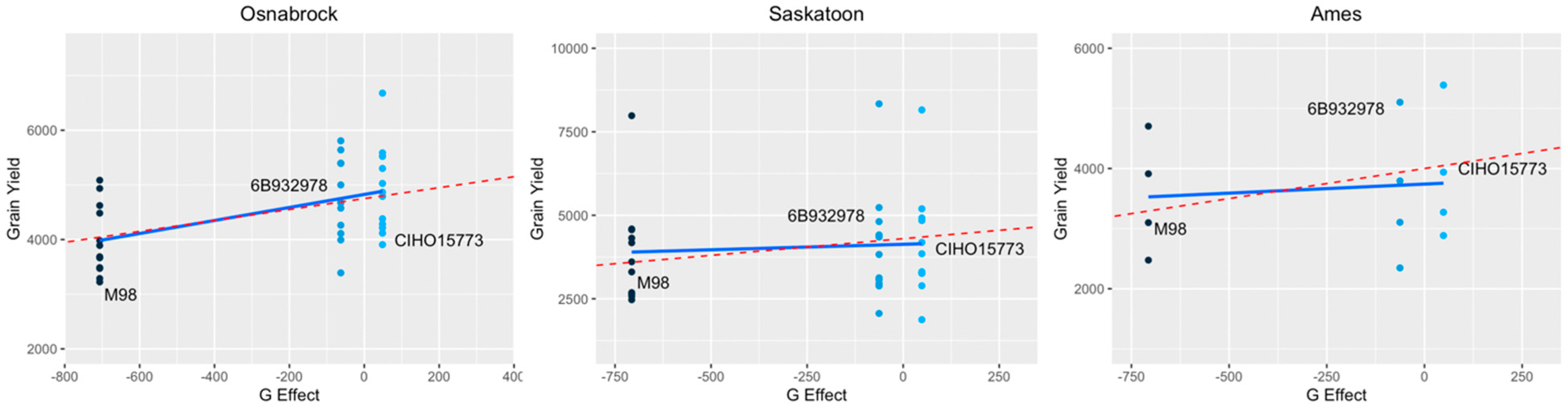
3.3. Insights into Pareto Optimality Tradeoff

The motivation behind looking at Pareto optimality is that there is a tradeoff between high precision and high RDVs, and that both are useful for discrimination in different ways. In this section, we aim to provide insights into the tradeoff between the Pareto optimal locations by reporting yield results for a small set of cultivars observed in three locations in each region, namely a location with high precision but a poor RDV (Saskatoon in MVN and Sterling in WRN), a location with low precision but a very good RDV (Osnabrock in MVN and Moses Lake in WRN), and a location with both low precision and a poor RDV (Ames in MVN and Bozeman in WRN). The selection of locations is based on the grain yield results shown in Figure 4.

We plot the observations for the three selected cultivars in the three locations where the x-axis shows the estimated main effect (G effect) of the cultivar, and the y-axis shows the observations in this location across all the years where it has been observed. Those plots are shown in Figure 5 and Figure 6 for the MVN and WRN regions, respectively. The plots also include the fitted line from the regression model (1), the slope of which is the RDV for the location (solid line) and expected slope of one (if RDV = 0).

Based on the results reported in Figure 4, we expect Osnabrock and Saskatoon to be useful in different ways, and Ames not to be very helpful when discriminating the three cultivars. For these locations, the variance difference is not very apparent but the difference in slope is clear (see Figure 5). Osnabrock has the highest RDV, represented as the steepest slope in the regression line, and even though the variance is too large to draw conclusions from a single location, there appears to be a better separation between the three cultivars when observed in Osnabrock versus the other two locations. On the other hand, as can be seen from Figure 5, Saskatoon has a smaller variance than Osnabrock, which allows it to have a more precise estimation.

Similarly, based on the results reported in Figure 4, we would expect Moses Lake and Sterling to be useful in different ways and Bozeman to have less value. This is supported by the plots reported in Figure 6. Sterling has very small variance compared to Moses Lake, allowing us to obtain a more precise estimate, whereas Moses Lake retains the correct order of the best and worst observation for each cultivar but has high variance. Specifically, if we are to rely on only one location, the superior precision makes it easier to determine that WPBB259435 has lower yield than STEPTOE based on the observations in Sterling, whereas it is not possible to distinguish that SK76333 is better than STEPTOE based on Sterling, but it is more evident from the Moses Lake observations.

These observations are anecdotal, and the variance in each location is too large to draw conclusions based on a single location; nonetheless, these observations provide insights into why both high-precision and high-RDV locations have value when we need to discriminate the main effects of a set of genotypes.

4. Conclusions

We have analyzed the data to identify the discriminative locations from both the traditional precision perspective and the newly proposed relative discriminative value (RDV) that uses a regression model to determine which locations are most sensitive with respect to changes in the genetic main effects. An ideal location is a location that has a high positive RDV with a high p value so that we are confident in its significance, as well as high precision (low variance). However, we observed that no such ideal location exists in the data, as locations with a high RDV also tend to have high variance, and we expect this to be true for other MET data as well.

For a practitioner who wants to plan or even optimize a set of early-stage trial locations by screening out the poor cultivars, the primary takeaway observations are as follows:

• A discriminative location should not be defined only in terms of precision or equivalently low variance. Some high-variance locations are discriminative because they are sensitive to the main genotype effect and those will tend to have high variance.
• No location will maximize both precision and the RDV. Instead, there is a tradeoff that can be addressed through a Pareto optimization approach that considers precision and the RDV simultaneously and identifies a set of desirable locations from the perspective of discriminating genotype main effects.
• While there is no ideal location, the Pareto optimization does identify locations that could be excluded from the perspective of discriminating main effects. In our results for grain yield, half of the locations for both regions are found to be less useful.
• The selection of a high RDV versus low variance may depend on the trial stage and the number of observations available. When there is a substantial amount of data, increasing precision may be more important, as in such cases, it is more plausible that sufficient precision can be obtained to discriminate between cultivars with close main effects. Vice versa, when there is a small amount of data available, the biased estimate of the genotype difference that results from using high-RDV locations may be more useful to discriminate between such cultivars.

We conclude by observing that while we have focused exclusively on the discriminative value of locations in METs and found that precision and RDVs should be considered simultaneously when planning locations for trials, this should then be combined with other considerations, such as representativeness and repeatability. In addition, stability across environments can be assessed using AMMI and GGE approaches to identify locations with consistent G × E patterns [5]. In fact, the analysis discussed here should be considered complimentary to those other methods and applied at a different time in the process, that is, when planning locations for a trial rather than when analyzing the outcome of the trial.

References

1. Neyhart, J.L.; Gutierrez, L.; Smith, K.P. Optimizing the choice of test locations for multitrait genotypic evaluation. Crop Sci. 2022, 62, 192–202. [Google Scholar] [CrossRef]
2. Yan, W. GGE biplot: A Windows application for graphical analysis of multi environment trial data and other types of two- way data. Agron. J. 2001, 93, 1111–1118. [Google Scholar] [CrossRef]
3. Yan, W.; Kang, M.S. GGE Biplot Analysis: A Graphical Tool for Breeders, Geneticist, and Agronomists; CRC Press: Boca Raton, FL, USA, 2003. [Google Scholar]
4. Gauch, H.G., Jr. Statistical Analysis of Yield Trials by AMMI and GGE. Crop Sci. 2006, 46, 1488–1500. [Google Scholar] [CrossRef]
5. Gauch, H.G., Jr.; Piepho, H.-P.; Annicchiarico, P. Statistical Analysis of Yield Trials by AMMI and GGE: Further Considerations. Crop Sci. 2008, 48, 866–889. [Google Scholar] [CrossRef]
6. Yan, W.; Kang, M.S.; Ma, B.; Woods, S.; Cornelius, P.L. GGE Biplot vs. AMMI Analysis of Genotype-by-Environment Data. Crop Sci. 2007, 47, 643–653. [Google Scholar] [CrossRef]
7. Shahriari, Z.; Heidari, B.; Dadkhodale, A. Dissection of genotype × environment interactions for mucilage and seed yield in Plantago species: Application of AMMI and GGE biplot analyses. PLoS ONE 2018, 13, e0196095. [Google Scholar] [CrossRef] [PubMed]
8. Hassani, M.; Heidari, B.; Dadkhodale, A.; Stevanato, P. Genotype by environment interaction components underlying variations in root, sugar and white sugar yield in sugar beet (Beta vulgaris L.). Euphytica 2018, 214, 79. [Google Scholar] [CrossRef]
9. Bernardo, R. Breeding for Quantitative Traits in Plants, 2nd ed.; Stemma Press: Woodbury, MN, USA, 2010. [Google Scholar]
10. Vemireddy, H.; Olafsson, S. A Regression Approach to Identify Discriminating Locations. Crop Sci. 2022, 63, 598–612. [Google Scholar] [CrossRef]
11. Clark, S.A.; van der Werf, J. Genomic best linear unbiased prediction (gBLUP) for the estimation of genomic breeding values. Methods Mol. Biol. 2013, 1019, 321–330. [Google Scholar] [CrossRef] [PubMed]
12. Piepho, H.P.; Möhring, J.; Melchinger, A.E.; Büchse, A. BLUP for phenotypic selection in plant breeding and variety testing. Euphytica 2008, 161, 209–228. [Google Scholar] [CrossRef]
13. Chinchuluun, A.; Pardalos, P.M. A survey of recent developments in multiobjective optimization. Ann. Oper. Res. 2007, 154, 29–50. [Google Scholar] [CrossRef]
14. Mattson, C.A.; Messac, A. Pareto frontier based concept selection under uncertainty, with visualization. Optim. Eng. 2005, 6, 85–115. [Google Scholar] [CrossRef]
15. Cheng, D.; Yao, Y.; Liu, R.; Li, X.; Guan, B. Precision agriculture management based on a surrogate model assisted multiobjective algorithmic framework. Sci. Rep. 2023, 13, 1142. [Google Scholar] [CrossRef] [PubMed]
Figure 1. Illustration of the Pareto front set of location and the desirable set of locations. There are three locations on the Pareto frontier. Two more locations are then added. One of them has better precision than the average of the three locations, and the other has a better RDV than the average of the three locations. Both have an RDV that is not significantly different than the RDV of the closest location on the Pareto fronter.
Agronomy 15 00935 g001
Figure 2. Relative discriminative value and precision for grain protein and grain yield and grain protein in MVN region. Size of dots represent significance of RDV (highly significant means p value < 0.01, significant means 0.01 < p < 0.1, and insignificant means p > 0.1). Base location used for grain protein (left) is Osnabrock and base location used for grain yield (right) is Crookston (not displayed).
Agronomy 15 00935 g002
Figure 3. Relative discriminative value and precision for grain protein and grain yield and grain protein in WRN region. Size of dots represent significance of RDV (highly significant means p value < 0.01, significant means 0.01 < p < 0.1, and insignificant means p > 0.1). Base location used for grain protein (left) is Aberdeen and base location used for grain yield (right) is Pullman (not displayed).
Agronomy 15 00935 g003
Figure 4. Pareto optimal frontier (solid line) and set of locations desirable for discrimination (shaded area) for grain yield in the MVN region (left) and WRN region (right).
Agronomy 15 00935 g004
Figure 5. Comparison of three cultivars for grain yield that are all planted in Osnabrock, Saskatoon, and Ames (MVN region). Solid line shows regression line for location obtained from model (1), and dashed line is expected relationship between yield and genetic main effect (slope = 1).
Agronomy 15 00935 g005
Figure 6. Comparison of three cultivars for grain yield that are all planted in Moses Lake, Sterling, and Bozeman (WRN region). Solid line shows regression line for location obtained from model (1), and dashed line is expected relationship between yield and genetic main effect (slope = 1).
Agronomy 15 00935 g006