Abstract
This study investigates the early detection of sweet potato scab by using hyperspectral imaging and machine learning techniques. The research focuses on developing an accurate, economical, and non-destructive approach for disease detection and grading. Hyperspectral imaging experiments were conducted on two sweet potato varieties: Guangshu 87 (resistant) and Guicaishu 2 (susceptible). Data preprocessing included denoising, region of interest (ROI) selection, and average spectrum extraction, followed by dimensionality reduction using principal component analysis (PCA) and random forest (RF) feature selection. A novel dynamic grading method based on spectral-time data was introduced to classify the early stages of the disease, including the early latent and early mild periods. This method identified significant temporal spectral changes, enabling a refined disease staging framework. Key wavebands associated with sweet potato scab were identified in the near-infrared range, including 801.8 nm, 769.8 nm, 898.5 nm, 796.4 nm, and 780.5 nm. Classification models, including K-nearest neighbor (KNN), support vector machine (SVM), and linear discriminant analysis (LDA), were constructed to evaluate the effectiveness of spectral features. Among these classification models, the MSC-PCA-SVM model demonstrated the best performance. Specifically, the Susceptible Variety Disease Classification Model achieved an overall accuracy (OA) of 98.65%, while the Combined Variety Disease Classification Model reached an OA of 95.38%. The results highlight the potential of hyperspectral imaging for early disease detection, particularly for non-destructive monitoring of resistant and susceptible sweet potato varieties. This study provides a practical method for early disease classification of sweet potato scab, and future research could focus on real-time disease monitoring to enhance sweet potato crop management.
1. Introduction
Sweet potato (Ipomoea batatas L.) is an annual crop recognized for its high yield, stability, and ease of cultivation, making it an essential food and feed resource globally [1,2]. China stands as the largest producer of sweet potatoes, with a planting area of approximately 7.43 million hectares and an annual output of 110 million tons in 2023. Sweet potato scab is one of the three major diseases in southern China. The pathogen is Elsinoë batatas, which can infect sweet potato leaves and stems. The symptom of sweet potato scab disease is that the leaves show small red spots at the initial stage, gradually expanding with the growth of leaves, and finally forming gray-brown raised scabs, and the leaf veins bend inward in a knee-bending shape. The disease spots on the stems and vines are purple-brown round or oval cork-shaped scabs at the beginning and then may develop into depressions. In severe cases, multiple disease spots may connect to form flakes, while the milk on the vines of plants usually becomes scarce. The young shoots of severely infected plants will shrink and cannot extend normally. Scab can occur in the whole growth period of sweet potato. If it occurs in the early growth stage, the yield loss can reach 60~70% [3]. Therefore, early detection of sweet potato scab is crucial for effective disease management and sustainable agricultural practices.
Modern imaging technologies, such as RGB, multispectral, and hyperspectral imaging, have shown great potential in providing more objective, high-throughput, cost-effective, and non-destructive methods for plant disease assessment compared to traditional human visual evaluation techniques. These technologies have been widely applied in the early detection of plant diseases, offering significant advantages in accuracy and efficiency, which are crucial for timely disease management [4,5,6]. Among its applications, plant disease monitoring and identification are vital for ensuring crop health and maximizing yield [7]. Crops are subjected to different stresses to cause some subtle changes in their physiological and biochemical characteristics, which will reflect the subtle changes in spectral reflectance at different wavelengths, which provides a prediction index for the identification of crop diseases [8,9,10,11].
Several studies have successfully applied spectral analysis to plant disease detection. Romain Bebronne used reflectance and texture features of multispectral images to carry out a field near-end sensing of winter wheat smut spot, stripe rust, and brown rust and achieved an accurate estimation of disease severity [12]. Nguyen et al. used hyperspectral images for the identification of wavelength regions and the identification and classification of a disease-centered vegetation index for grapevine vein clearance virus (GVCV) [10]. Xie et al. demonstrated early detection of crown rot in wheat using HSI, linking spectral changes to photosynthetic activity and water absorption [4]. Zheng et al. identified the most sensitive bands for the detection of stripe rust in wheat at multiple growth stages, such as 460–720 nm in the early to middle growth stage, 568–709 nm, and 725–1000 nm in the middle and late growth stage [9]. Zhang et al. used vegetation indices PRI and anthocyanin reflectance index (ARI) at different growth stages to evaluate the severity of wheat stripe rust disease [13]. Fazari et al. inoculated olives artificially and divided them into a control group and fungal groups. Using vis/NIR hyperspectral images and ResNet101 architecture, infected olives were effectively detected with high sensitivity [14]. Fajardo et al. used a partial least squares penalized logistic regression (pls-plr) model and hyperspectral double plot to evaluate the effect of HSI on the early detection of banana black leaf spot disease. The accuracy of their work in detecting black leaf spot disease in the early stage was 98% [15]. Zhang et al. used leaf-level vegetation index (VI) data extracted from hyperspectral data to detect bacterial leaf spot (BLS) disease on tomato plants at presymptomatic stages and differentiate bacterial disease spots from abiotic leaf spots [16]. Bao et al. explored the potential of using hyperspectral imaging combined with deep learning techniques for the early detection of sugarcane anthracnose and mosaic disease, achieving detection accuracies exceeding 90% [17]. Many studies have shown that hyperspectral sensors can be used for non-invasive and objective observation of plant physiological changes caused by pathogens and have the advantages of accuracy, efficiency, and cost-effectiveness. Hyperspectral sensors are valuable tools for plant disease management and monitoring at different scales from tissue to canopy. The main contributions of this paper are as follows:
- By comparing the spectral differences between resistant and susceptible sweet potato varieties after inoculation, this study reveals the varietal differences in response mechanisms to early-stage scab disease and identifies key sensitive spectral bands associated with sweet potato scab.
- A dynamic spectral-time grading method for early asymptomatic disease classification is proposed, integrated with machine learning models. The accuracy and performance improvements of the proposed method are validated.
- Addressing the challenge of limited sample sizes, this study explores the use of region of interest (ROI) extraction and data augmentation techniques to expand the dataset, enhancing the model’s generalization ability and classification accuracy.
2. Materials and Methods
2.1. Cultivation and Inoculation of Sweet Potato
Experiments were conducted using the sweet potato scab-resistant variety Guangshu 87 (GS87) and the susceptible variety Guicaishu 2 (GCS2). The cultivation took place in pots at the Guangdong Academy of Agricultural Sciences, with the plants divided into two equal groups: a control group and an experimental group. The pathogen (Elsinoë batatas) was isolated from scab lesions on infected sweet potato leaves. After purification, a conidial suspension was prepared at a concentration of 3 × 10⁴ conidia/mL. For artificial inoculation, the conidial suspension was sprayed onto the leaf surfaces of test plants using a handheld sprayer. Following inoculation, the plants were covered with plastic bags to maintain high humidity and placed in a growth chamber under controlled conditions (25 °C, 12 h light/dark cycle, 90% relative humidity) to facilitate infection [18]. Figure 1 shows healthy and infected sweet potato plants.
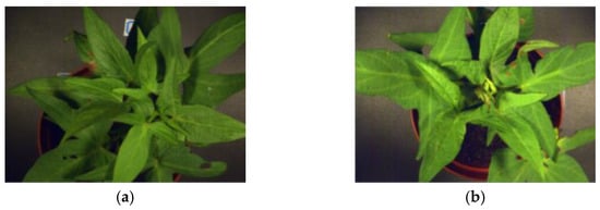
Figure 1.
Early sweet potato plants under different treatments. (a) Healthy plants; (b) infected plants.
2.2. Hyperspectral Image Acquisition and Preprocessing
The hyperspectral imager used in this study was the SOC710-VP, with a spectral range of 400–1000 nm, a spectral resolution of 2.1 nm, and 128 bands. Imaging was conducted at a resolution of 696 × 520 pixels in a light-controlled room, isolated from natural light. The camera was mounted horizontally on a tripod, positioned 0.4 m above the potted sweet potato samples, and illuminated by two 500 W halogen lamps placed at a 45-degree angle. The setup remained fixed throughout the imaging cycle, with samples photographed against a white background.
The two sweet potato varieties, resistant and susceptible, were divided into a control group and a treatment group, with three replicates in each group, totaling twelve plants. Spectral preprocessing, including dark current correction and reflectance conversion, was performed using the SRAnal710e Version 3.0 software provided by the manufacturer. During the filming period, there were no obvious disease spots on the infected plants. The second day after vaccination is considered as the first day of infection and filming begins from that day onwards. The shooting conditions at that time are shown in Figure 2.
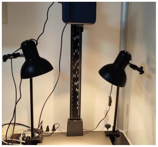
Figure 2.
Hyperspectral shooting location and equipment, including halogen lamp, tripod, hyperspectral camera.
The process of converting digital number (DN) values to reflectivity enhances the interpretation of hyperspectral data, as reflectivity more accurately represents the chemical properties of the observed objects. This radiometric calibration involves using the measured intensity (iP), dark current (iD), and white light reference values (iw) is used to calculate the reflectance (rp) at each spatial position (x, y) and wavelength λ [19,20].
2.3. Spectral Data Extraction and Masking
The hyperspectral images were processed using the spectral radiance analysis toolkit v3.5 provided by the SOC710E equipment (AZUP International, Beijing, China). Initially, the raw image data were input in cube format and output in float32 format after preprocessing. This preprocessing included dark current correction and reflectance conversion, which are essential for accurately representing the chemical properties of the observed objects [21]. In addition to the target leaves, the hyperspectral images also contain background information that significantly differs from the leaf spectra in Figure 3. After preprocessing, the region of interest (ROI) tool in ENVI5.6 was used to extract the irregularly shaped leaves from the calibrated potted sweet potato plants. The hyperspectral data corresponding to these leaves were then isolated for further analysis [22]. A total of 5–10 spectral groups were extracted from each hyperspectral image and saved in TIFF format. After outlier elimination, the dataset contained 248 images of healthy leaves and 289 images of inoculated leaves, for a total of 527 images. The hyperspectral data of the target leaves were then successfully isolated and prepared for further analysis in Figure 4.
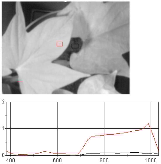
Figure 3.
Average spectrum and background average spectrum curve of a certain area of collected leaves. The red curve represents the average spectrum of leaves within the region, while the black curve represents the average spectrum of the background within the region.
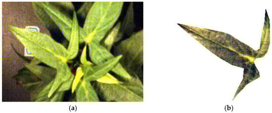
Figure 4.
Extraction and mask processing of region of interest in leaves. (a) An RGB image of the sweet potato leaf; (b) the picture after region of interest cropping.
2.4. Spectral Denoising Preprocessing
In the process of collecting data with a spectral camera, in addition to the characteristic information of the sample data, there are also some irrelevant noise and information. Denoising helps improve the quality of hyperspectral data, providing a more reliable basis for subsequent data analysis and model building [23,24,25,26]. Denoising is helpful to improve the quality of hyperspectral data and provides a more reliable basis for subsequent data analysis and model building. Based on different spectral application scenarios, spectral preprocessing methods are mainly divided into the baseline correction method, scattering correction method, smoothing method, signal enhancement method, and noise elimination method [27]. Moving average (MA) smoothing is a simple yet effective method for reducing high-frequency random noise in spectral data. It operates by replacing each spectral data point with the average of its neighboring points within a defined window size. This technique is particularly effective for smoothing fluctuations in the reflectance curve caused by random noise, while preserving the overall trend of the signal. Savitzky–Golay (SG) smoothing is a widely used noise reduction method, which can effectively eliminate the white noise in the spectrum data, but it is invalid for low-frequency and broadband noise [28,29]. Multiple scatter correction (MSC) is mainly used to eliminate the effects of uneven distribution of solid particles, particle size, surface scattering, and light path changes on the diffuse reflectance spectrum [30].
2.5. Dynamic Grading Method for Early Disease Stages
Early plant disease detection is challenging because most vegetation is in the asymptomatic or mild symptom stage during the early stages of infection. Traditional disease classification methods, which rely on the size of disease spots, are not applicable at this stage. However, partial spectral characteristics change significantly due to the onset of infection. Based on dynamic spectral classification over time, it is possible to identify the onset and stages of early disease. In this study, based on the early characteristics of sweet potato scab, the disease progression is classified into two initial stages after inoculation: the early latent period and the early mild period. To evaluate these stages, two grading methods are employed. The first method is a dynamic grading approach based on spectral-time data analysis. The core principle of this approach is to analyze the spectral data and identify significant changes over time. This dynamic classification method aims to determine the transition points between the latent stage and other stages through data-driven analysis, without relying solely on subjective experimental decisions. By identifying spectral differences at key wavelengths and analyzing time-related changes, we can establish objective thresholds that delineate the disease’s progression. This method is particularly valuable for capturing subtle spectral variations that may not be easily visible to the human eye or through conventional disease scoring techniques. The second grading method is based on the experimental setup, wherein disease stages are classified into two periods based on a simpler, manual division of time and treatment conditions. This approach serves as a straightforward comparison to the dynamic grading method and provides additional validation for the data-driven approach.
2.6. Data Augmentation
Data augmentation is a technique commonly employed in small sample learning to enhance model performance by increasing the diversity of available data. By expanding the dataset, this method allows for more robust cross-validation, enabling the evaluation of model performance across different data subsets [31,32]. In this study, two data augmentation strategies—average spectral enhancement and random noise enhancement—are applied together to improve the reliability of spectral data for model training. Average spectral enhancement generates smoother and denoised spectral data by randomly selecting samples and calculating their mean values. This approach helps reduce noise and improve the signal-to-noise ratio in the spectral data. Random noise enhancement, on the other hand, introduces disturbance into the data by adding Gaussian noise, thereby simulating real-world measurement variations. This technique generates perturbations that closely resemble natural data fluctuations, making the augmented data more representative of actual conditions. By combining these two methods, the dataset is enriched, improving the generalization ability of the model and making it more robust to real-world variations in spectral data. The training set and test are divided into 8:2 sections. In the dynamic grading training set, the susceptible variety Gui15-12 includes 138 healthy control samples, 94 early mild stage samples, and 52 early latent stage samples. After data augmentation, each category contains 200 samples.
2.7. Dimension Reduction Method
Due to hyperspectral data having a large number of bands, each band corresponds to a feature, so feature selection can help us select the most representative and important features from a large number of bands to reduce the data dimension and improve the performance and interpretability of the model. PCA guarantees the main features and structure of the data by retaining the maximum variance in the dataset, reducing the complexity of the data, to help us extract the principal components from a large amount of spectral information and better understand the data structure and relationship [33]. Random forest is an integrated learning method, which is composed of multiple decision trees, and each tree is trained using a randomly selected feature subset [34,35,36]. In random forest, the importance of feature selection is measured by calculating the impact of each feature on the accuracy of the model. In general, the more important the features used to build the tree, the greater their contribution to the model. After selecting the characteristic wavelength, the optimal combination and number of characteristic bands are selected by cross-validation, which can improve the accuracy and reduce the overfitting of the model [37].
2.8. Disease Classification Modeling Method
Support vector machine (SVM) is a binary classification algorithm based on supervised learning. It uses statistical learning theory to classify data by finding the hyperplane with the largest interval to achieve an excellent classification effect [38,39]. The core idea of SVM is to project data into high-dimensional feature space through non-linear mapping and perform linear classification in this high-dimensional space to achieve the purpose of non-linear classification in the original space. In this study, the grid search method is used to realize the superparameter optimization of SVM to build a leaf disease recognition and classification model.
K-nearest neighbors (KNN) is a neighbor classification algorithm. To determine the category of unknown samples, the distance between unknown samples and all known samples is calculated by taking all known samples as a reference, and K known samples nearest to the unknown samples are selected [40,41]. According to the voting rule of the majority, the unknown samples and the K nearest samples with more categories are classified into one category. The K value is usually odd. To better determine the size of the K value, this study uses the method of cross-validation to select the appropriate K value [42].
Linear discriminant analysis (LDA) is a supervised learning algorithm, which is mainly used for data classification and dimensionality reduction [43,44]. The core idea of LDA is to project the data into a low-dimensional space so that the projected data are as compact as possible within the category and as separate as possible between categories. Specifically, LDA attempts to find a set of linear transformations so that the transformed data have the maximum degree of separation between classes and the minimum intra-class dispersion in the new feature space.
3. Results
3.1. Spectral Data Analysis and Statistical Test
Due to the limitations of the SOC710E device, the spectrum beyond 960 nm exhibits significant noise. As a result, bands after 960 nm were removed, and 116 bands from 400 nm to 960 nm were retained as the effective spectral range.
Figure 5 shows that there is minimal spectral change in the visible light region (450 nm to 700 nm) during the early stages of disease. Spectral characteristics in this range primarily depend on chlorophyll content, which absorbs radiation in the regions around 450 nm and 670 nm, creating an absorption valley. A green reflection peak is formed due to the low absorption and transmission of green leaves, resulting in a healthy appearance. When affected by disease, this peak shifts from the blue light direction towards the red light direction. However, no significant changes were observed in the visible light spectrum, suggesting that early scab disease does not significantly impact chlorophyll content.
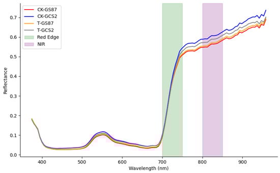
Figure 5.
Average spectra and sensitive bands of resistant variety GS87 and susceptible variety GCS2 under different treatments.
In the near-infrared region, the spectral characteristics of healthy crops are influenced by internal leaf structure. Pathogen inoculation disturbs water metabolism and damages the leaf cell structure, reducing the reflective ability of the leaves and decreasing near-infrared radiation. A “red-edge effect” in the near-infrared region, caused by changes in chlorophyll content, was also observed. Reflectance spectra of healthy leaves were slightly higher than those of infected leaves.
T-tests were conducted on the near-infrared and red-edge bands for the healthy (CK, control) and treatment (T) groups of the resistant variety GS87 and the susceptible variety GCS2. As shown in Table 1, significant differences were observed in the red-edge band of the susceptible variety GCS2 (p = 0.039), while no significant differences were found in the resistant variety GS87 (p = 0.535).

Table 1.
Internal t-test of GS87 (CK and T) and GCS2 (CK and T).
In the analysis of variance (ANOVA), the visible band exhibited non-homogeneous variance (Levene’s test, p < 0.05) as shown in Table 2. Welch’s ANOVA revealed significant differences between varieties (p < 0.001), but no significant differences between treatments (p = 0.628). In the two-way ANOVA, the interaction between varieties and treatments was not significant (p = 0.001).
Table 2.
Visible band of Welch’s ANOVA.
In contrast, the near-infrared band showed homogeneous variance (Levene’s test, p = 0.072). Standard ANOVA revealed significant differences between varieties (p < 0.001) and days (p < 0.001) but no significant differences among treatments (p = 0.411) as shown in Table 3. Multivariate analysis of variance (MANOVA) revealed significant interactions between varieties and treatments (p = 0.036) and between varieties and days (p = 0.011), highlighting the combined effects of these factors on spectral variance.
Table 3.
NIR band of ANOVA.
3.2. Dynamic Classification of Early Disease
The goal of dynamic disease classification is to identify the time points corresponding to the incubation and mild disease stages by analyzing spectral changes. Significant differences in spectral bands between the control and treatment groups were compared on a day-to-day basis, and the ratio of significant bands (p < 0.05) was calculated. A ratio greater than 50% was used as the indicator for the early incubation period.
Figure 6 shows that the significant differences in spectral bands between the control and treatment groups are greater than those observed between two consecutive days within the control group. Additionally, the proportion of significant bands between the control and treatment groups progressively increases over time. On Day 1, the proportion of significant bands exceeded 50%, and Day 1 was chosen as the classification point between the early incubation period and the control group.
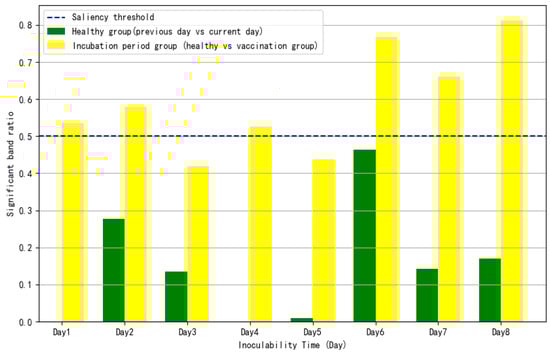
Figure 6.
Comparison of the proportion of significant bands between dynamic characteristic health and early latency groups.
Figure 7 presents a day-to-day comparison within the treatment group. The proportion of significant bands on Day 3, Day 4, and Day 6 exceeded 40%, with Day 6 showing more than 50%. As spectral differences diminished, it can be inferred that the disease had reached short-term stability and entered the next disease stage. The spectral differences significantly decreased after Day 4 and Day 6, indicating that these time points mark the onset of the early mild period.
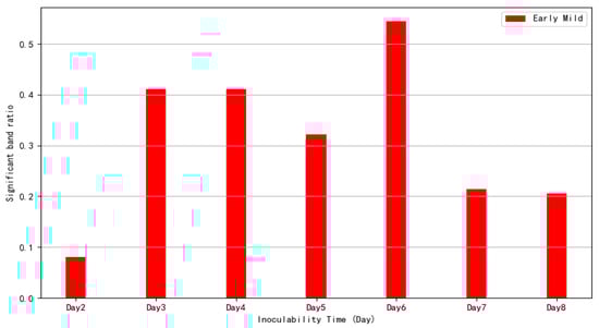
Figure 7.
Significant band proportion change in the early mild phase of dynamic characteristics.
3.3. Spectral Data Preprocessing
Savitzky–Golay (SG) smoothing, moving average (MA) filtering, and multivariate scattering correction (MSC) were applied to the spectral data of the susceptible variety GCS2 in both the control and treatment groups. Based on the spectral-time dynamic grading method, the treatment group was classified into appropriate disease stages.
After testing the performance of each method, the MSC method was selected due to its superior prediction effect in subsequent modeling. Figure 8 shows the average spectra of the control and treatment groups after applying the three denoising methods. The spectra for the treatment group were averaged according to the disease stages identified through dynamic grading, preserving the differences between disease stages while reducing noise.
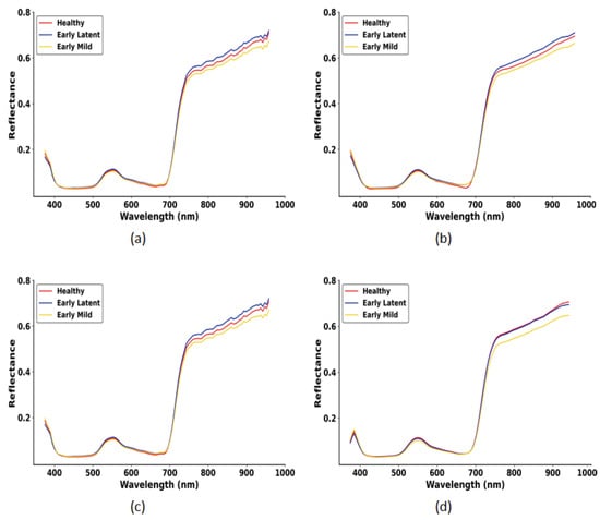
Figure 8.
Average spectra for control and treatment groups (graded by spectral-time dynamic classification). (a) Original average spectrum; (b) the SG noise reduction method; (c) the MSC noise reduction method; (d) the MA noise reduction method.
3.4. Hyperspectral Image Dimensionality Reduction
Hyperspectral data, characterized by high dimensionality and redundancy, require dimensionality reduction to extract meaningful features. In this study, the effective spectral range spans from 400 to 900 nm, comprising 113 bands [45]. Principal component analysis (PCA) was applied to the spectral data for dimensionality reduction through feature extraction. The first two principal components explained 40% (PC1) and 27% (PC2) of the variance, respectively. A two-dimensional scatter plot of PC1 and PC2 (Figure 9) shows the distribution of disease stages. The healthy stage and early incubation period exhibit relatively close clustering but remain distinguishable. In contrast, the early mild stage forms a dense, distinct cluster, separated from the other two stages. These results indicate that the extracted principal components effectively contribute to the classification of disease stages.
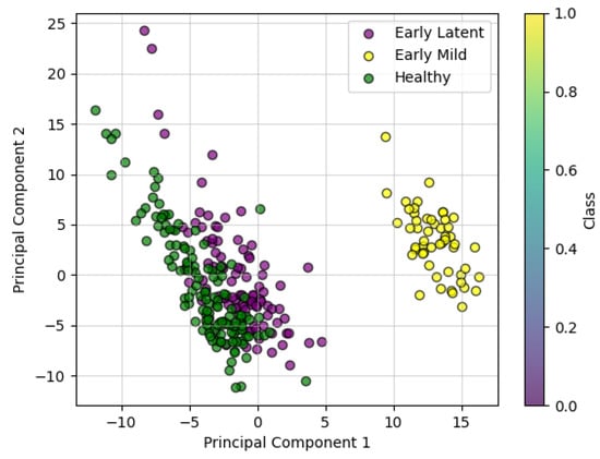
Figure 9.
Two-dimensional principal component analysis of PC1 and PC2.
Additionally, random forest (RF) was used for feature selection to identify the most relevant spectral bands. Cross-validation was applied to select an optimal set of feature vectors. The importance scores for each spectral band are illustrated in Figure 10. The top five most important bands were identified as the 84th, 78th, 102nd, 83rd, and 80th bands, corresponding to wavelengths of 801.8 nm, 769.8 nm, 898.5 nm, 796.4 nm, and 780.5 nm, respectively. These bands align with the spectral differences observed between healthy and infected leaves in the average spectrum, where significant variations are evident in the near-infrared region. Furthermore, the top 20 important bands were concentrated within the wavelength range of 764.5–936.5 nm, highlighting the critical role of the near-infrared spectrum in distinguishing disease stages.
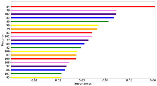
Figure 10.
Top 20 characteristic importance maps of random forest (RF).
3.5. Results of Susceptible Variety Disease Classification Models
Machine learning classification models can be divided into two categories: single classifiers and ensemble classifiers. Single classifiers, such as logistic regression, support vector machine (SVM), and decision trees, achieve classification through individual algorithms. Ensemble classifiers, such as random forest (RF) and extreme random forests, combine multiple base classifiers to improve classification performance.
Based on the cross-validation results and data augmentation methods described earlier, the most effective scheme was selected for subsequent classification modeling [46]. Figure 11 shows the confusion matrix for the prediction accuracy of each model under PCA and RF processing. As the number of selected features increased, the model’s accuracy improved, stabilizing between 0.93 and 0.99.
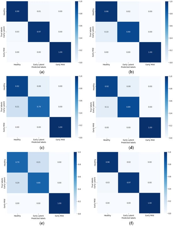
Figure 11.
The test set confusion matrix of the disease grade discrimination results of the model after MSC noise reduction. (a) PCA-SVM; (b) PCA-LDA; (c) PCA-KNN; (d) RF-SVM; (e) RF-LDA; (f) RF-KNN.
Among the models tested, the PCA-SVM model demonstrated the best classification performance. Hierarchical cross-validation revealed that the average accuracy of the test set was 98.20%, with a standard deviation of 1.53%. The accuracy for individual categories was 0.99 for the healthy group, 0.97 for the early latent stage, and 1.00 for the early mild stage. The classification accuracy for the early mild stage was consistently 100% across all models. The primary variation in accuracy among models was observed in the healthy group and early latent stage.
To optimize model performance and mitigate overfitting, the optimal number of features was determined through cross-validation using the random forest feature selection method. Figure 12 illustrates the model accuracy for different numbers of selected features. As the number of features increased, the model’s accuracy improved significantly, stabilizing between 0.93 and 0.99. This suggests a strong correlation between the selected spectral wavelengths and disease recognition performance. The positive relationship between the number of features and classification accuracy indicates that increasing the number of selected wavelengths enhances the model’s effectiveness.
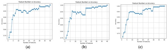
Figure 12.
Line graph of feature quantity and accuracy under different models. (a) RF-SVM; (b) RF-LDA; (c) RF-KNN.
In this study, 15 characteristic wavelengths with the most optimal phenotypic performance were selected for use in the RF-KNN model. The overall accuracy (OA) and kappa coefficients for each model are summarized in Table 4. The overall accuracy of all models ranged from 83.11% to 98.65%, with standard deviations ranging from 0.6% to 4.2%.
Table 4.
OA and kappa of test set and validation set of each disease classification model.
3.6. Results of Combined Variety Disease Classification Models
To further analyze the impact of resistant and susceptible varieties on disease classification, the control and treatment groups of the resistant varieties were incorporated into the dataset. Figure 13 presents the confusion matrix showing the prediction accuracy of each model under PCA and RF feature selection processing.
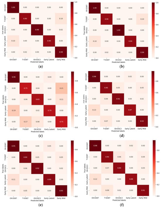
Figure 13.
The test set confusion matrix of the variety and disease classification model after MSC noise reduction. (a) PCA-SVM; (b) PCA-LDA; (c) PCA-KNN; (d) RF-SVM; (e) RF-LDA; (f) RF-KNN.
Among the models tested, the PCA-SVM model demonstrated the best classification performance following parameter optimization. Hierarchical cross-validation revealed an average test set accuracy of 96.25%, with a standard deviation of 0.36%. The classification accuracy for the resistant variety control group was 1.00, that of the treatment group was 0.90, and for the susceptible variety, the value for the control group was 0.98. The accuracy for the early incubation period was 0.90, and that of the early mild period was 0.98.
Table 5 summarizes the overall accuracy (OA) and kappa coefficients for each model. The total accuracy of all models ranged from 81.54% to 95.38%, with standard deviations from 0.36% to 1.72%. These results indicate that, while the classification models performed well in distinguishing most categories, further optimization is required, particularly for the resistant variety treatment group and the early incubation period of susceptible varieties, to enhance classification accuracy.
Table 5.
OA and kappa of test set and validation set of each variety and disease classification model.
4. Discussion
In this study, we focused on the early detection of sweet potato scab disease using hyperspectral imaging. Given the limited research on early-stage detection of this disease in sweet potatoes, our findings offer valuable insights into this underexplored area.
The results indicate that early-stage disease affects spectral responses in the red-edge region, particularly in the susceptible variety GCS2. The significant difference observed in the red-edge band (p = 0.039) suggests that early infection impacts chlorophyll content, which is reflected in this spectral region. In contrast, the near-infrared band, influenced by leaf water content and internal structure, showed no significant differences at this stage, indicating that these factors remain relatively stable in the early progression of the disease. For the resistant variety GS87, no significant spectral differences were observed, suggesting that this variety maintains spectral stability during early disease stages, consistent with its strong resistance. Previous studies on other crops have shown that spectral shifts in the visible and near-infrared regions are key indicators of early disease stages, particularly in susceptible varieties. The lack of significant differences in GS87 further highlights its potential for disease resistance, while the response of GCS2 underscores the importance of chlorophyll content and photosynthetic efficiency in early-stage detection.
Early plant disease detection is challenging because most vegetation remains asymptomatic or exhibits mild symptoms during the early stages of infection. Traditional disease classification methods, which rely on the size of disease spots, are ineffective during this phase. However, partial spectral characteristics change significantly due to the onset of infection. Using dynamic spectral classification over time, it is possible to identify the onset and progression of early disease. The proportion of significant bands between the control and treatment groups increases as the disease advances, although this trend is not always consistent, suggesting that the mechanisms driving disease dynamics may vary over time. Once the disease reaches a stable phase, the difference in spectral characteristics between the control and treatment groups begins to decrease, indicating that the disease has entered a stable stage. These findings suggest that spectral features can serve as reliable early disease detection methods.
Table 6 presents a comparison of dynamic grading using the optimal classification model without data enhancement. The results indicate that the accuracy of the two dynamic disease classification methods based on spectral time is higher than that of manual classification. Furthermore, the accuracy of each model improves, demonstrating that the dynamic classification approach is effective in enhancing the accuracy of early disease detection. However, none of the models achieved optimal classification performance for the GCS2 healthy group and early latent period. This could be attributed to the fact that, although interference from leaf edges was removed when selecting the region of interest, the selection of large portions of the leaf area may have masked subtle spectral changes associated with early-stage disease. As a result, the spectral characteristics of early disease were less pronounced across the entire spectrum.
Table 6.
Accuracy of different classification methods in disease classification model.
PCA identifies the principal components (PCs) that explain the most variance in the data, effectively reducing the number of features while preserving the essential structure of the dataset. By focusing on the most significant components, PCA filters out noise and irrelevant information, improving the signal-to-noise ratio and enhancing model performance.
Despite its high accuracy, this study has limitations. The controlled environment used in the experiments could introduce bias, as they were conducted indoors under stable lighting conditions. Field validation is necessary to account for environmental variability. Additionally, the current model focuses on E. batatas, and future work should extend to other sweet potato pathogens (e.g., Fusarium spp.). To address these issues, we plan to develop low-cost hyperspectral sensors for field deployment, expand the dataset to include multiregional sweet potato varieties, and explore fusion with thermal or LiDAR data for multimodal disease assessment.
5. Conclusions
This study demonstrates the potential of hyperspectral imaging combined with machine learning techniques for the early detection and classification of sweet potato scab. Significant spectral differences between resistant and susceptible sweet potato varieties were observed, particularly in the near-infrared region (764.5–936.5 nm), which were strongly correlated with disease progression. A dynamic spectral-time grading method was developed to accurately classify early latent and mild disease stages, significantly improving classification performance. To address limited sample sizes, data augmentation techniques were applied, enhancing model training and accuracy. Additionally, key spectral bands for disease detection were identified through dimensionality reduction techniques and feature selection, further refining the model’s sensitivity. The findings highlight the potential of hyperspectral imaging for early disease detection and its applicability in large-scale field monitoring. Future research could expand this approach by integrating remote sensing technologies and extending it to the detection of other sweet potato diseases across different growth stages.
Author Contributions
Conceptualization, X.N., F.Z., Z.W., H.Z., X.Y. and L.H.; methodology, X.N., F.Z., H.Z. and X.Y.; software, X.N.; validation, X.N., Q.X., Z.D. and F.Z.; formal analysis, X.N., Q.X., Z.D. and X.Y.; investigation, X.N., Q.X., F.T. and X.D.; resources, F.T., X.D., Z.W. and L.H.; data curation, X.N., F.T., X.D. and L.H.; writing—original draft preparation, X.N.; writing—review and editing, X.N., Q.X., Z.D., F.Z., X.Y. and L.H.; visualization, X.N.; supervision, X.N., X.Y. and L.H.; project administration, X.N., Z.W. and L.H.; funding acquisition, L.H. All authors have read and agreed to the published version of the manuscript.
Funding
This work was supported by grants from the earmarked fund for CARS-10-Sweetpotato, the Project of Science and Technology of Guangdong Province (No. 2023B1212060038) and Sweetpotato Potato Innovation Team of Modern Agricultural Industry Technology System in Guangdong Province (2023KJ111).
Data Availability Statement
The data that support the findings of this study are available from the corresponding author, Lifei Huang, upon reasonable request.
Acknowledgments
Thank you to mentors Lifei Huang and Xuejun Yue for providing financial and technical support.
Conflicts of Interest
The authors declare no conflicts of interest.
References
- Vaddi, R.; Phaneendra Kumar, B.L.N.; Manoharan, P.; Agilandeeswari, L.; Sangeetha, V. Strategies for dimensionality reduction in hyperspectral remote sensing: A comprehensive overview. Egypt. J. Remote Sens. Space Sci. 2024, 27, 82–92. [Google Scholar] [CrossRef]
- Hennessy, A.; Clarke, K.; Lewis, M. Hyperspectral Classification of Plants: A Review of Waveband Selection Generalisability. Remote Sens. 2020, 12, 113. [Google Scholar] [CrossRef]
- Sapakhova, Z.; Raissova, N.; Daurov, D.; Zhapar, K.; Daurova, A.; Zhigailov, A.; Zhambakin, K.; Shamekova, M. Sweet Potato as a Key Crop for Food Security under the Conditions of Global Climate Change: A Review. Plants 2023, 12, 2516. [Google Scholar] [CrossRef]
- Sapakhova, Z.; Islam, K.R.; Toishimanov, M.; Zhapar, K.; Daurov, D.; Daurova, A.; Raissova, N.; Kanat, R.; Shamekova, M.; Zhambakin, K. Mulching to improve sweet potato production. J. Agr. Food Res. 2024, 15, 101011. [Google Scholar] [CrossRef]
- Xu, Y.; Liu, Y.; Wang, Y.; Liu, Y.; Zhu, G. Whole-Genome Sequencing and Genome Annotation of Pathogenic Elsinoë batatas Causing Stem and Foliage Scab Disease in Sweet Potato. J. Fungi 2024, 10, 882. [Google Scholar] [CrossRef]
- Xie, Y.; Plett, D.; Evans, M.; Garrard, T.; Butt, M.; Clarke, K.; Liu, H. Hyperspectral imaging detects biological stress of wheat for early diagnosis of crown rot disease. Comput. Electron. Agric. 2024, 217, 108571. [Google Scholar] [CrossRef]
- Xie, Y.; Plett, D.; Liu, H. Detecting Crown Rot Disease in Wheat in Controlled Environment Conditions Using Digital Color Imaging and Machine Learning. Agriengineering 2022, 4, 141–155. [Google Scholar] [CrossRef]
- Almoujahed, M.B.; Rangarajan, A.K.; Whetton, R.L.; Vincke, D.; Eylenbosch, D.; Vermeulen, P.; Mouazen, A.M. Detection of fusarium head blight in wheat under field conditions using a hyperspectral camera and machine learning. Comput. Electron. Agric. 2022, 203, 107456. [Google Scholar] [CrossRef]
- Thomas, S.; Kuska, M.T.; Bohnenkamp, D.; Brugger, A.; Alisaac, E.; Wahabzada, M.; Behmann, J.; Mahlein, A. Benefits of hyperspectral imaging for plant disease detection and plant protection: A technical perspective. J. Plant Dis. Prot. 2018, 125, 5–20. [Google Scholar] [CrossRef]
- Nguyen, C.; Sagan, V.; Maimaitiyiming, M.; Maimaitijiang, M.; Bhadra, S.; Kwasniewski, M.T. Early Detection of Plant Viral Disease Using Hyperspectral Imaging and Deep Learning. Sensors 2021, 21, 742. [Google Scholar] [CrossRef]
- Wu, G.; Fang, Y.; Jiang, Q.; Cui, M.; Li, N.; Ou, Y.; Diao, Z.; Zhang, B. Early identification of strawberry leaves disease utilizing hyperspectral imaging combing with spectral features, multiple vegetation indices and textural features. Comput. Electron. Agric. 2023, 204, 107553. [Google Scholar] [CrossRef]
- Bhujade, V.G.; Sambhe, V. Role of digital, hyper spectral, and SAR images in detection of plant disease with deep learning network. Multimed. Tools Appl. 2022, 81, 33645–33670. [Google Scholar] [CrossRef]
- Wan, L.; Li, H.; Li, C.; Wang, A.; Yang, Y.; Wang, P. Hyperspectral Sensing of Plant Diseases: Principle and Methods. Agronomy 2022, 12, 1451. [Google Scholar] [CrossRef]
- Bebronne, R.; Carlier, A.; Meurs, R.; Leemans, V.; Vermeulen, P.; Dumont, B.; Mercatoris, B. In-field proximal sensing of septoria tritici blotch, stripe rust and brown rust in winter wheat by means of reflectance and textural features from multispectral imagery. Biosyst. Eng. 2020, 197, 257–269. [Google Scholar] [CrossRef]
- Zheng, Q.; Huang, W.; Cui, X.; Dong, Y.; Shi, Y.; Ma, H.; Liu, L. Identification of Wheat Yellow Rust Using Optimal Three-Band Spectral Indices in Different Growth Stages. Sensors 2018, 19, 35. [Google Scholar] [CrossRef]
- Fazari, A.; Pellicer-Valero, O.J.; Gómez-Sanchıs, J.; Bernardi, B.; Cubero, S.; Benalia, S.; Zimbalatti, G.; Blasco, J. Application of deep convolutional neural networks for the detection of anthracnose in olives using VIS/NIR hyperspectral images. Comput. Electron. Agric. 2021, 187, 106252. [Google Scholar] [CrossRef]
- Ugarte Fajardo, J.; Bayona Andrade, O.; Criollo Bonilla, R.; Cevallos Cevallos, J.; Mariduena Zavala, M.; Ochoa Donoso, D.; Vicente Villardón, J.L. Early detection of black Sigatoka in banana leaves using hyperspectral images. Appl. Plant Sci. 2020, 8, e11383. [Google Scholar] [CrossRef] [PubMed]
- Zhang, X.; Vinatzer, B.A.; Li, S. Hyperspectral imaging analysis for early detection of tomato bacterial leaf spot disease. Sci. Rep. 2024, 14, 27614–27666. [Google Scholar] [CrossRef]
- Bao, D.; Zhou, J.; Bhuiyan, S.A.; Adhikari, P.; Tuxworth, G.; Ford, R.; Gao, Y. Early detection of sugarcane smut and mosaic diseases via hyperspectral imaging and spectral-spatial attention deep neural networks. J. Agric. Food Res. 2024, 18, 101369. [Google Scholar] [CrossRef]
- Zhang, X.; Chen, J.; Fang, B.; Wang, Z.; Yao, Z.; Huang, L. Identification of the pathogen causing sweet potato scab in Guangdong and resistance evaluation of main domestic leaf-vegetable sweet potato germplasm resources. J. Plant Prot. 2021, 48, 298–304. [Google Scholar] [CrossRef]
- Liu, H.; Bruning, B.; Garnett, T.; Berger, B. The Performances of Hyperspectral Sensors for Proximal Sensing of Nitrogen Levels in Wheat. Sensors 2020, 20, 4550. [Google Scholar] [CrossRef] [PubMed]
- Asadzadeh, S.; de Souza Filho, C.R. A review on spectral processing methods for geological remote sensing. Int. J. Appl. Earth Obs. Geoinf. 2016, 47, 69–90. [Google Scholar] [CrossRef]
- Ram, B.G.; Oduor, P.; Igathinathane, C.; Howatt, K.; Sun, X. A systematic review of hyperspectral imaging in precision agriculture: Analysis of its current state and future prospects. Comput. Electron. Agric. 2024, 222, 109037. [Google Scholar] [CrossRef]
- Chylla, R.A.; Van Acker, R.; Kim, H.; Azapira, A.; Mukerjee, P.; Markley, J.L.; Storme, V.; Boerjan, W.; Ralph, J.; Great, L.B.R.C. Plant cell wall profiling by fast maximum likelihood reconstruction (FMLR) and region-of-interest (ROI) segmentation of solution-state 2D ¹H−¹³C NMR spectra. Biotechnol. Biofuels 2013, 6, 45. [Google Scholar] [CrossRef] [PubMed]
- Vidal, M.; Amigo, J.M. Pre-processing of hyperspectral images. Essential steps before image analysis. Chemom. Intell. Lab. Syst. 2012, 117, 138–148. [Google Scholar] [CrossRef]
- Rinnan, Å.; Berg, F.V.D.; Engelsen, S.B. Review of the most common pre-processing techniques for near-infrared spectra. TrAC Trends Anal. Chem. 2009, 28, 1201–1222. [Google Scholar] [CrossRef]
- Zhang, Q.; Xiao, J.; Tian, C.; Chun Wei Lin, J.; Zhang, S. A robust deformed convolutional neural network (CNN) for image denoising. CAAI Trans. Intell. Technol. 2023, 8, 331–342. [Google Scholar] [CrossRef]
- Noshiri, N.; Beck, M.A.; Bidinosti, C.P.; Henry, C.J. A comprehensive review of 3D convolutional neural network-based classification techniques of diseased and defective crops using non-UAV-based hyperspectral images. Smart Agric. Technol. 2023, 5, 100316. [Google Scholar] [CrossRef]
- Gowen, A.; Xu, J.; Herrero-Langreo, A. Comparison of spectral selection methods in the development of classification models from visible near infrared hyperspectral imaging data. J. Spectr. Imaging 2019, 8, a4. [Google Scholar] [CrossRef]
- Gao, W.; Cheng, X.; Liu, X.; Han, Y.; Ren, Z. Apple firmness detection method based on hyperspectral technology. Food Control 2024, 166, 110690. [Google Scholar] [CrossRef]
- Zheng, K.; Zhang, X.; Tong, P.; Yao, Y.; Du, Y. Pretreating near infrared spectra with fractional order Savitzky–Golay differentiation (FOSGD). Chin. Chem. Lett. 2015, 26, 293–296. [Google Scholar] [CrossRef]
- Li, C.; Wang, X.; Chen, L.; Zhao, X.; Li, Y.; Chen, M.; Liu, H.; Zhai, C. Grading and Detection Method of Asparagus Stem Blight Based on Hyperspectral Imaging of Asparagus Crowns. Agriculture 2023, 13, 1673. [Google Scholar] [CrossRef]
- Liu, X.; An, H.; Cai, W.; Shao, X. Deep learning in spectral analysis: Modeling and imaging. TrAC Trends Anal. Chem. 2024, 172, 117612. [Google Scholar] [CrossRef]
- Alaa Hussein, O.; Salih Mahdi, M. Review on Detection of Rice Plant Leaves Diseases Using Data Augmentation and Transfer Learning Techniques. Iraqi J. Comput. Inform. 2023, 49, 30–40. [Google Scholar] [CrossRef]
- Zhao, B.; Dong, X.; Guo, Y.; Jia, X.; Huang, Y. PCA Dimensionality Reduction Method for Image Classification. Neural Process. Lett. 2022, 54, 347–368. [Google Scholar] [CrossRef]
- Peng, W.; Karimi Sadaghiani, O. A review on the applications of machine learning and deep learning in agriculture section for the production of crop biomass raw materials. Energy Sources Part A Recovery Util. Environ. Eff. 2023, 45, 9178–9201. [Google Scholar] [CrossRef]
- Anowar, F.; Sadaoui, S.; Selim, B. Conceptual and empirical comparison of dimensionality reduction algorithms (PCA, KPCA, LDA, MDS, SVD, LLE, ISOMAP, LE, ICA, t-SNE). Comput. Sci. Rev. 2021, 40, 100378. [Google Scholar] [CrossRef]
- Li, Y.; Xu, X.; Wu, W.; Zhu, Y.; Yang, G.; Yang, X.; Meng, Y.; Jiang, X.; Xue, H. Hyperspectral Estimation of Chlorophyll Content in Grape Leaves Based on Fractional-Order Differentiation and Random Forest Algorithm. Remote Sens. 2024, 16, 2174. [Google Scholar] [CrossRef]
- Ihalainen, O.; Sandmann, T.; Rascher, U.; Mõttus, M. Illumination correction for close-range hyperspectral images using spectral invariants and random forest regression. Remote Sens. Environ. 2024, 315, 114467. [Google Scholar] [CrossRef]
- Bachhal, P.; Kukreja, V.; Ahuja, S.; Lilhore, U.K.; Simaiya, S.; Bijalwan, A.; Alroobaea, R.; Algarni, S. Maize leaf disease recognition using PRF-SVM integration: A breakthrough technique. Sci. Rep. 2024, 14, 10219. [Google Scholar] [CrossRef]
- Prince, R.H.; Mamun, A.A.; Peyal, H.I.; Miraz, S.; Nahiduzzaman, M.; Khandakar, A.; Ayari, M.A. CSXAI: A lightweight 2D CNN-SVM model for detection and classification of various crop diseases with explainable AI visualization. Front. Plant Sci. 2024, 15, 1412988. [Google Scholar] [CrossRef] [PubMed]
- Tu, B.; Wang, J.; Kang, X.; Zhang, G.; Ou, X.; Guo, L. KNN-Based Representation of Superpixels for Hyperspectral Image Classification. IEEE J. Sel. Top. Appl. Earth Obs. Remote Sens. 2018, 11, 4032–4047. [Google Scholar] [CrossRef]
- Huang, K.; Li, S.; Kang, X.; Fang, L. Spectral–Spatial Hyperspectral Image Classification Based on KNN. Sens. Imaging 2016, 17, 1. [Google Scholar] [CrossRef]
- Cheng, H. KNN-SVM Classifiers in Complex Diagnosis. J. Phys. Conf. Ser. 2024, 2694, 12081. [Google Scholar] [CrossRef]
- Fabiyi, S.D.; Murray, P.; Zabalza, J.; Ren, J. Folded LDA: Extending the Linear Discriminant Analysis Algorithm for Feature Extraction and Data Reduction in Hyperspectral Remote Sensing. IEEE J. Sel. Top. Appl. Earth Obs. Remote Sens. 2021, 14, 12312–12331. [Google Scholar] [CrossRef]
- Jia, S.; Zhao, Q.; Zhuang, J.; Tang, D.; Long, Y.; Xu, M.; Zhou, J.; Li, Q. Flexible Gabor-Based Superpixel-Level Unsupervised LDA for Hyperspectral Image Classification. IEEE Trans. Geosci. Remote Sens. 2021, 59, 10394–10409. [Google Scholar] [CrossRef]
Disclaimer/Publisher’s Note: The statements, opinions and data contained in all publications are solely those of the individual author(s) and contributor(s) and not of MDPI and/or the editor(s). MDPI and/or the editor(s) disclaim responsibility for any injury to people or property resulting from any ideas, methods, instructions or products referred to in the content. |
© 2025 by the authors. Licensee MDPI, Basel, Switzerland. This article is an open access article distributed under the terms and conditions of the Creative Commons Attribution (CC BY) license (https://creativecommons.org/licenses/by/4.0/).