Evaluation of Shelf Life Prediction for Broccoli Based on Multispectral Imaging and Multi-Feature Data Fusion

Abstract

Broccoli is a highly nutritious vegetable that is favored worldwide. Assessing and predicting the shelf life of broccoli holds considerable importance for effective resource optimization and management. The physicochemical parameters and spectral characteristics of broccoli are important indicators partially reflecting its shelf life. However, few studies have used spectral image information to predict and evaluate the shelf life of broccoli. In this study, multispectral imaging combined with multi-feature data fusion was used to predict and evaluate the shelf life of broccoli. Spectral data and textural features were extracted from multispectral images of broccoli and fused with the physicochemical parameters for analysis. Savitzky–Golay (SG) convolution smoothing and standard normal variate (SNV) and normalization (Norm) preprocessing methods were employed to preprocess the original spectral data and textural features, while a successive projection algorithm (SPA) was used to extract relevant feature bands. The physicochemical parameters for broccoli shelf life were predicted using three methods: support vector regression (SVR), random forest classification (RF), and 2D convolutional neural network (2D-CNN) models. Broccoli shelf life prediction models were evaluated using three classification methods: RF, 1D-CNN, and 2D-CNN. The results demonstrate that, among the models used for predicting and evaluating the shelf life of broccoli, the SPA+SG+RF classification model employing fused data Type C achieves the highest accuracy. Specifically, this method achieves accuracies of 88.98% and 88.64% for the training and validation sets, respectively. Multi-feature data fusion of spectral image information and physical and chemical parameters were combined with different machine learning methods to predict and evaluate the shelf life of broccoli.

1. Introduction

Broccoli (Brassica oleracea L. var. Italica) belongs to the Cruciferae family and the Brassica genus. It is rich in various nutrients and bioactive compounds that benefit human health, making it widely favored by consumers [1]. Broccoli is widely grown worldwide, with China as the leading producer. According to the 2023 statistics from the Food and Agriculture Organization (FAO), the harvested area in China reached 498,862 hectares. However, the post-harvest storage of broccoli faces numerous challenges, including temperature and humidity variation. Unfavorable storage conditions accelerate wilting and yellowing, leading to a rapid loss of nutrients and a decline in its functional properties [2]. The demand for rapid and non-destructive quality assessment of broccoli has become increasingly urgent.

The quality of broccoli is closely linked to its shelf life [3,4]. Correct assessment of the shelf life and quality of broccoli is vital for effective resource management and use, and it has a key role in economic estimation. Various methods have been adopted to extend its shelf life, including controlling storage temperature, humidity, and chemical treatments. For example, Patil et al. [5], Paulsen et al. [6], and Zhan et al. [7] have investigated strategies to control post-harvest storage temperature, while Pintos et al. [8] and Loi et al. [9] have evaluated the effects of light variables in storage environments. Xu et al. [10] and Cai et al. [11] have applied chemical treatments to improve broccoli’s shelf life. However, the shelf life of broccoli is most commonly evaluated by experienced professionals using time-consuming, labor-intensive, subjectively biased sensory methods. Therefore, precise determination of broccoli’s shelf life and quality throughout the supply chain and supermarket retail process is beneficial for effective resource management.

Spectral imaging technology, which integrates traditional imaging with spectral techniques, enables the simultaneous acquisition of spatial and spectral information from samples, providing advantages such as speed and accuracy without damaging the product [12]. Indeed, spectral imaging combined with machine learning and deep learning algorithms has been widely applied for agricultural product quality and shelf-life assessment [13,14]. For example, Sricharoonratana et al. [15] used hyperspectral imaging combined with partial least squares regression and partial least squares discriminant analysis to accurately predict and classify cake shelf life. Doing so demonstrated the feasibility of combining hyperspectral imaging with machine learning for shelf life prediction. Meanwhile, Siripatrawan and Makino [16] developed a backpropagation neural network model for the rapid and accurate evaluation of sausage shelf life, showing the effectiveness of combining hyperspectral imaging with deep learning algorithms to evaluate shelf life. Shao et al. [17] constructed a Library for Support Vector Machines (LIBSVM) model to analyze winter jujube shelf life, achieving accuracies of 89% and 91% for medium and mature jujubes, respectively, and demonstrating the potential of hyperspectral imaging combined with neural networks to monitor post-harvest shelf life. Furthermore, Tang et al. [18] and Hu et al. [19] established random forest (RF) and support vector machine (SVM) machine learning models to evaluate tea quality. They confirmed that combining spectral imaging with machine learning may be used to effectively assess tea quality. Collectively, these studies validate the practical application of spectral imaging technology for shelf life prediction. However, changes in the physical appearance of food products during the shelf life are also important factors in evaluating quality.

Yin et al. [20] integrated texture features, which are key phenotypic features, with spectral information to classify tea quality. Moreover, Zhang et al. [21] employed near-infrared hyperspectral imaging with spectral and texture features for the non-destructive determination of fat and moisture content in salmon. Due to the cost-effectiveness of multispectral imaging, many researchers have also combined it with machine learning platforms to create rapid and non-destructive quality assessment tools for agricultural products. For example, Lytou et al. [22] combined multispectral imaging with deep learning for rapid microbial prediction in fish fillets across the supply chain. Meanwhile, Zhang et al. [23] established a model for predicting dietary fiber content variation at different growth stages of Chinese cabbage by combining multispectral imaging with chemometric methods, achieving an R² of 0.9023. This method can be further adapted to provide technical support for produce sorting and grading. Yang et al. [24] utilized multispectral imaging to rapidly assess seed moisture content, with a backpropagation neural network model achieving an accuracy of 90.1%, providing an effective monitoring method for seed storage. Duan et al. [25] developed a model for detecting pepper diseases using multispectral imaging combined with texture features. Their findings confirm that integrating texture features with spectral data is more effective than relying on spectral data alone, further validating the feasibility of multi-feature data fusion technology. Therefore, using multispectral imaging technology combined with multi-feature data fusion and machine learning to predict and evaluate the shelf life of broccoli is feasible. This provides a basis for studying chlorophyll and other physicochemical parameters, as well as for determining the shelf life of broccoli.

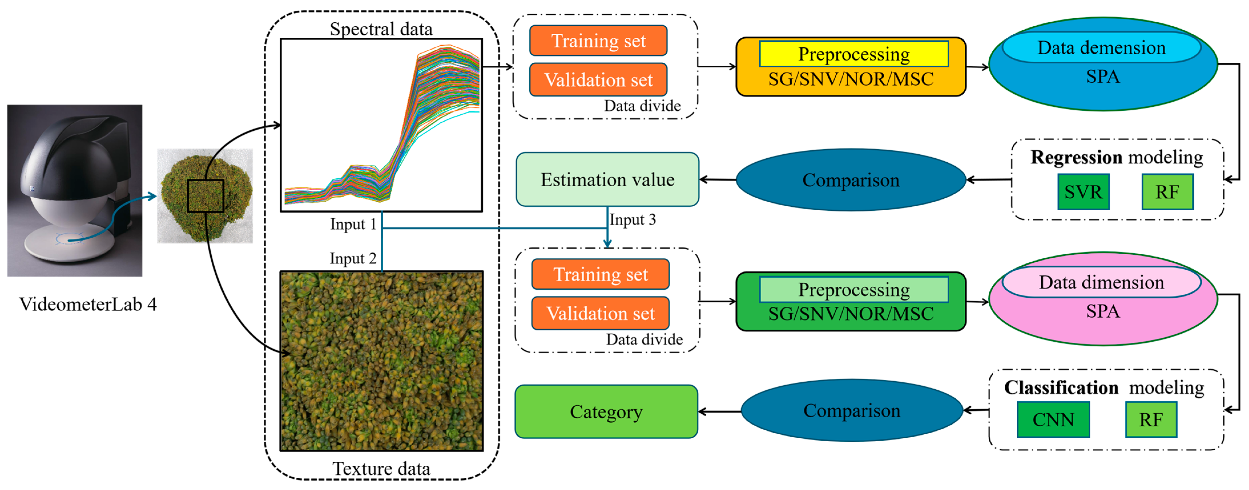
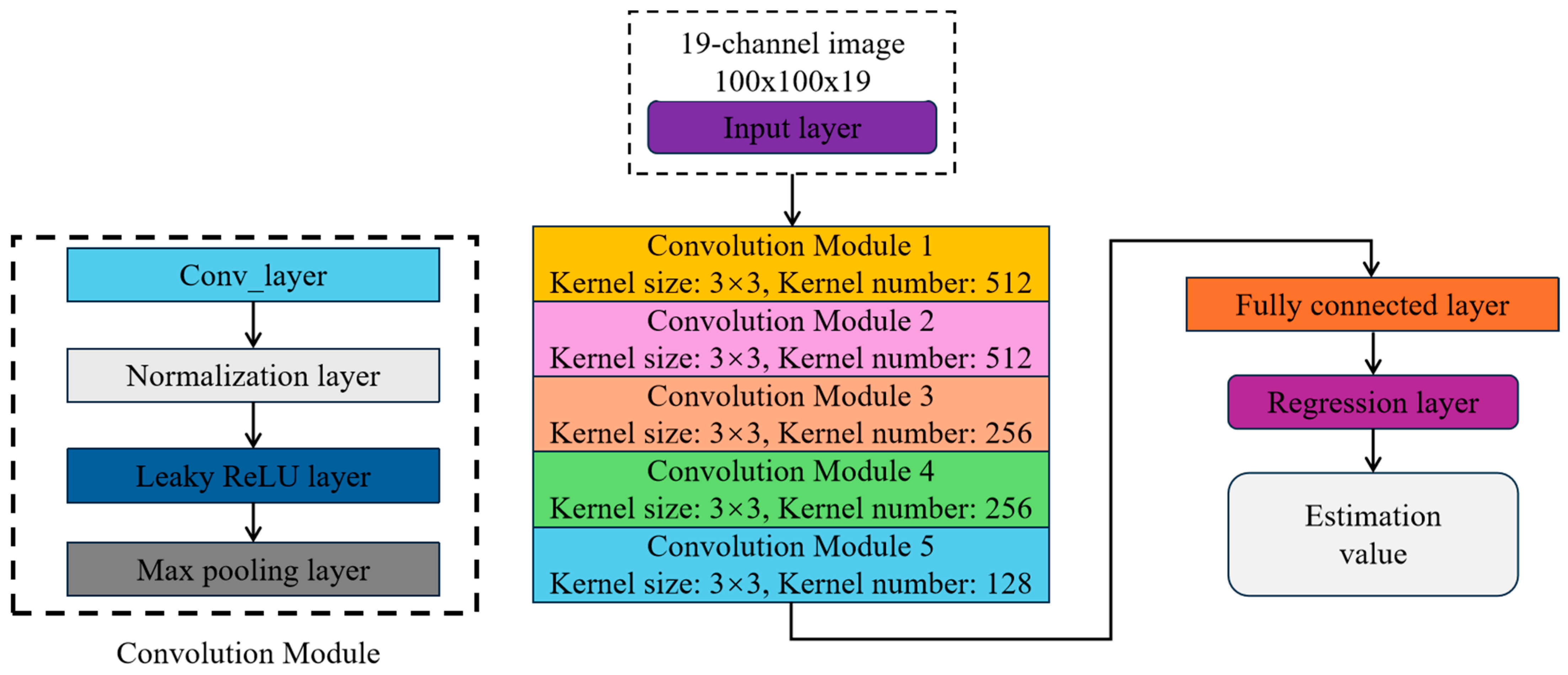
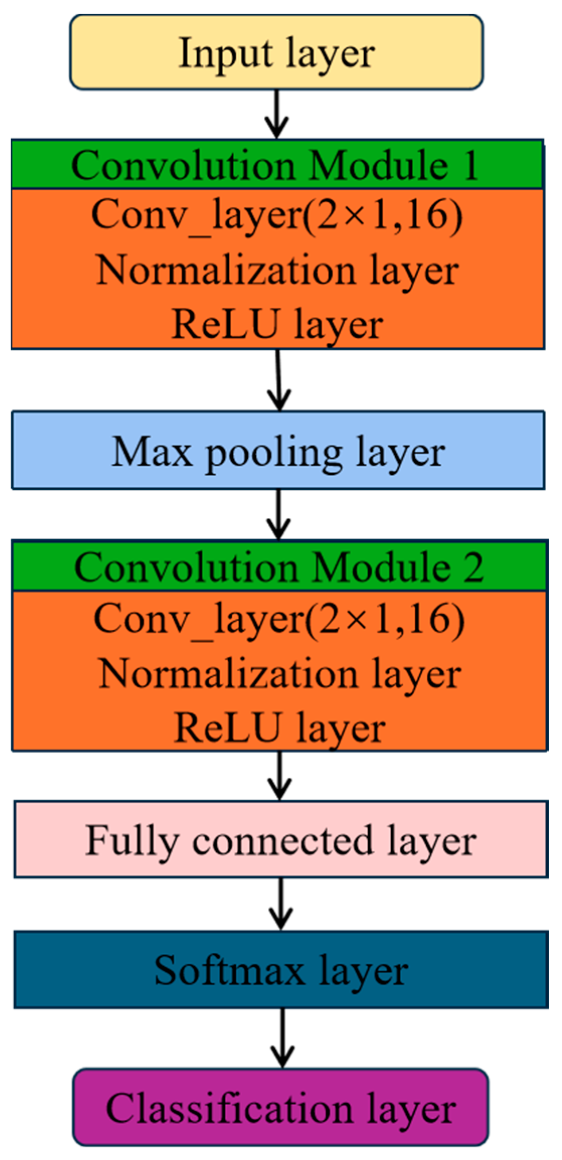
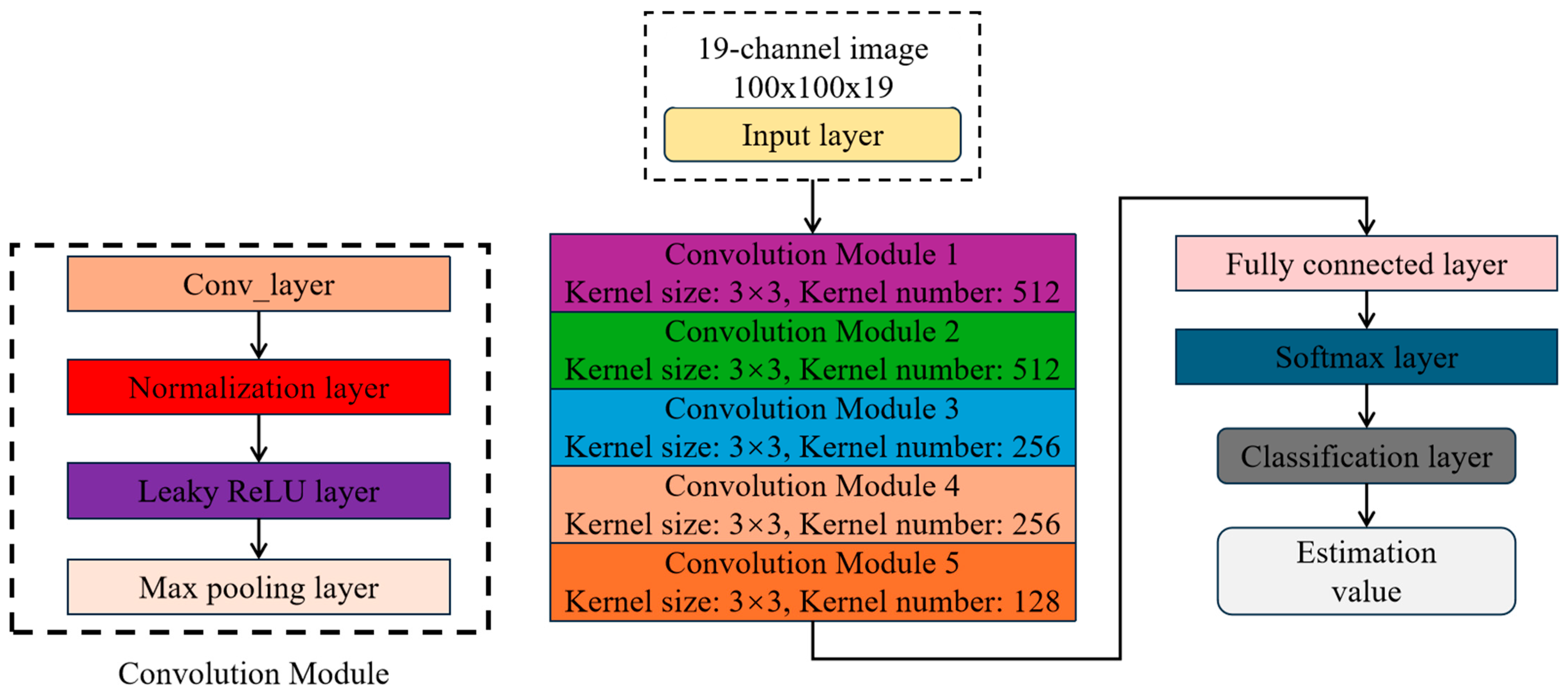
Therefore, this study combined multispectral imaging technology with multi-feature data fusion and machine learning to develop a rapid and accurate prediction and evaluation model for broccoli shelf life. Specifically, spectral data and texture features were extracted from multispectral images, and the moisture content and photosynthetic pigments (including chlorophyll and carotenoids) of broccoli were measured. Using these data, support vector regression (SVR), RF, and 2D convolutional neural networks (2D-CNN) are incorporated into prediction models for the physicochemical parameters of broccoli throughout its shelf life. Additionally, 1D-CNN, RF, and 2D-CNN were used to develop models for evaluating the shelf life. Subsequently, the prediction and evaluation of broccoli’s shelf life were systematically analyzed, validating the feasibility of combining multispectral imaging technology with multi-feature data fusion and machine learning to achieve rapid, accurate, and non-destructive shelf life prediction and evaluation.

2. Materials and Methods

2.1. Broccoli Samples

The broccoli samples were collected in November 2023 from the experimental field of Tianjin Huierjia Seed Industry Co., Ltd., located in Tianjin, China (117.260132° N, 38.89377801° E). The soil in the experimental field is saline-alkali, and the winter environment is cold and dry. A total of 110 mature commercial varieties were selected as experimental materials. The selected samples were stored in an environment with a room temperature of 10 °C, and data were collected from the broccoli samples every 24 h for a total of 10 collections. As shown in Figure 1, all samples were used to acquire multispectral images and relevant physicochemical parameters.

2.2. Multispectral Image Acquisition

A VideometerLab 4 device (manufactured in Denmark and distributed by Beijing Bopute Technology Co., Ltd., Beijing, China), a spectral imaging device used for the rapid determination of crop chemical composition, color, and texture, was used to obtain multispectral images of broccoli samples. Before scanning, it was turned on and run for 30 min to ensure a stable light environment. It can capture images under 19 different wavelengths of a light-emitting diode (LED) flashlight (365 nm, 405 nm, 430 nm, 450 nm, 470 nm, 490 nm, 515 nm, 540 nm, 570 nm, 590 nm, 630 nm, 645 nm, 660 nm, 690 nm, 780 nm, 850 nm, 880 nm, 940 nm, and 970 nm), including visible light imaging, ultraviolet (UV) imaging, and near-infrared (NIR) imaging. Each pixel in the acquired image represents a reflectance spectrum. During the experiment, the broccoli samples were placed inside the enclosed integrating sphere of the device and scanned for 5–10 s for spectral image acquisition. Multispectral images were collected from the 110 broccoli samples every 24 h, resulting in a total of 1100 multispectral images over 10 days, which were used as the dataset. The overall workflow of this study is shown in Figure 2, illustrating the process from data acquisition and preprocessing to model development.

2.3. Determination of Physicochemical Parameters

The measured physicochemical parameters included moisture content and photosynthetic pigments (chlorophyll and carotenoids). Moisture content was calculated as the ratio of the dry weight to the fresh weight of the broccoli samples. Fresh broccoli samples were placed in an oven at 105 °C to terminate enzymatic activity and then dried in an oven at 65 °C until a constant weight was achieved. The moisture content was calculated using Equation (1) as proposed by Zhang et al. [26]:

$$\mathrm{y}={\displaystyle \frac{w_1-w_2}{w_1}}\times 100\%,$$

(1)

where $\mathrm{y}$ represents the moisture content, $w_1$ represents the fresh weight mass of the broccoli sample, and $w_2$ represents the dry weight mass of the broccoli sample.

According to the absorption of visible light by the chlorophyll extraction solution, absorbance A at a specific wavelength was determined using a spectrophotometer, and the content of each pigment in the extraction solution was calculated using Equations (2)–(5), as proposed by Zhang et al. [26]:

$$\mathrm{C}\mathrm{h}\mathrm{l}\mathrm{o}\mathrm{r}\mathrm{o}\mathrm{p}\mathrm{h}\mathrm{y}\mathrm{l}\mathrm{l} \mathrm{a}=\left(12.7\times {\mathrm{A}}_{663}-2.69\times {\mathrm{A}}_{645}\right)\times \mathrm{V}/(\mathrm{W}\times 1000),$$

(2)

$$\mathrm{C}\mathrm{h}\mathrm{l}\mathrm{o}\mathrm{r}\mathrm{o}\mathrm{p}\mathrm{h}\mathrm{y}\mathrm{l}\mathrm{l} \mathrm{b}=\left(22.88\times {\mathrm{A}}_{645}-4.67\times {\mathrm{A}}_{663})\times \mathrm{V}/(\mathrm{W}\times 1000)\right.,$$

(3)

$$\mathrm{C}\mathrm{h}\mathrm{l}\mathrm{o}\mathrm{r}\mathrm{o}\mathrm{p}\mathrm{h}\mathrm{y}\mathrm{l}\mathrm{l}=\left(8.04\times {\mathrm{A}}_{663}+20.69\times {\mathrm{A}}_{645}\right)\times \mathrm{V}/(\mathrm{W}\times 1000),$$

(4)

$$\mathrm{C}\mathrm{a}\mathrm{r}\mathrm{o}\mathrm{t}\mathrm{e}\mathrm{n}\mathrm{o}\mathrm{i}\mathrm{d}\mathrm{s}=4.695\times {\mathrm{A}}_{470}-0.268\times (\mathrm{a}+\mathrm{b}),$$

(5)

where V = 10 and W = 0.2. Absorbance A is only measured at two specific wavelengths in the extraction solution to determine the contents of chlorophyll and carotenoids; the concentration is obtained based on the absorbance coefficient of chlorophyll and carotenoids at that wavelength.

Surface impurities were removed from broccoli samples (0.2 g). The tissue was cleaned, finely diced, placed in a 50 mL centrifuge tube containing 10 mL of mixed extraction solution (absolute ethanol/acetone = 1:1), and incubated in the dark until the sample cleared. Absorbance was measured at 663 nm, 645 nm, and 470 nm. The absorbance values at the three wavelengths are denoted as A663, A645, and A470, respectively.

2.4. Data Preprocessing

2.4.1. Spectral Data and Texture Feature Extraction

The compositions of the target area and background in the multispectral images differed, and further analysis required the binarization and separation of the target area and background in the multispectral image to isolate meaningful information. Therefore, based on Matlab R2021a software, the 1100 multispectral images were segmented using the OTSU algorithm to separate the target region (broccoli) from the background. The spectral image information of the target region, including spectral data and texture features, was then extracted. Texture feature extraction involved the use of the grey-level co-occurrence matrix (GLCM) method to extract four texture features: contrast, correlation, energy, and homogeneity, along with the local binary pattern (LBP) method to extract parameters from LBP1 to LBP59. Parameters with a value of 0 were deleted, resulting in 16 texture features.

2.4.2. Spectral Data Preprocessing

Various data preprocessing methods were applied to the extracted raw spectral data to improve the conventional data preprocessing methods, including convolution smoothing, multiplicative scatter correction, and normalization. In this experiment, four preprocessing methods—Savitzky–Golay (SG) convolution smoothing [27], standard normal variate (SNV) [28], normalization (Norm) [29], and multiplicative scatter correction (MSC) [30]—were used to preprocess the raw spectral data.

2.4.3. Data Dimensionality Reduction

Selecting characteristic bands is crucial for improving model accuracy, reducing computational load, and minimizing the risk of overfitting. In this experiment, the successive projection algorithm (SPA), a forward feature variable selection method that extracts effective characteristic bands and addresses the issue of collinearity between variables, was used to extract characteristic bands from the raw spectral data.

2.5. Model Establishment

2.5.1. Establishing the Regression Model

Using the spectral data, SVR and RF algorithms were used to construct prediction models for water, chlorophyll, and carotenoid content. SVR is an extension of SVM, a supervised machine learning algorithm with good performance widely used in regression and classification tasks for spectral data analysis [31]. RF is a powerful and flexible machine learning algorithm with strong performance in regression and classification tasks, and its performance is predominantly led by basic unit decision trees [32]. The model input comprised preprocessed spectral data and physicochemical parameters, with the physicochemical parameters serving as dependent variables for each model.

The regression model for shelf life prediction based on multispectral imaging adopts a 2D-CNN algorithm. This model uses multispectral images as input, with an input layer consisting of 19 channels of 100 × 100 pixels. The basic framework of the 2D-CNN model comprised an input layer, five convolutional modules, a fully connected layer, and a regression layer. Each convolutional module consisted of a convolutional layer, an activation layer, a normalization layer, and a pooling layer. The numbers of convolutional kernels in the respective convolutional layers of the five modules were 512, 512, 256, 256, and 128; all were 3 × 3 pixels. Batch normalization was applied in the normalization layer, a leaky rectified linear unit (ReLU) activation function was used in the activation layer, and max pooling was used in the pooling layer. The structure of the 2D-CNN model used to predict the physicochemical parameters of broccoli using multispectral images is illustrated in Figure 3.

The broccoli dataset was randomly divided into training and validation sets at a ratio of 8:2 to establish the regression models. The model performance was evaluated based on R2 and root mean square deviation (RMSE) values calculated using Equations (6) and (7) as reported by Khodabakhshian et al. [33]:

$${\mathrm{R}}^2={\displaystyle \frac{{\sum \left({\widehat{\mathrm{y}}}_{\mathrm{i}}-\stackrel{-}{\mathrm{y}}\right)}^2}{{\sum \left({\mathrm{y}}_i-\stackrel{-}{\mathrm{y}}\right)}^2}},$$

(6)

$$\mathrm{R}\mathrm{M}\mathrm{S}\mathrm{E}=\sqrt{{\displaystyle \frac{{\sum }_{\mathrm{i}=1}^{\mathrm{n}}{\left({\widehat{\mathrm{y}}}_{\mathrm{i}}-{\mathrm{y}}_i\right)}^2}{\mathrm{n}}},}$$

(7)

where ${\mathrm{y}}_i$ represents the actual value, ${\widehat{\mathrm{y}}}_{\mathrm{i}}$ represents the estimated value, $\stackrel{-}{\mathrm{y}}$ represents the mean of the actual values, and $\mathrm{n}$ represents the number of samples.

2.5.2. Establishing the Classification Model

The multi-feature data fusion in this study integrates features from different data sources (spectral data, texture features, and physicochemical parameters) to form a new feature vector, which serves as the input data for the classification model. The shelf life of broccoli was classified using 1D-CNN and RF algorithms employing multi-feature fusion data. CNNs have been widely used as algorithms for spectral classification. The 1D-CNN comprises an input layer, two convolutional modules, a pooling layer, a fully connected layer, a loss function layer, and a classification layer. Each convolutional module comprises a convolutional layer, an activation layer, and a normalization layer. The convolutional layers in the two modules consist of 16 convolutional kernels with a size of 2 × 1 and a stride of 1. The ReLU activation function was used in the activation layer; batch normalization was applied in the normalization layer, and maximum pooling was used in the pooling layer. Figure 4 shows the structure of the 1D-CNN classification model employing the multi-feature fusion data.

A 2D-CNN algorithm model employing spectral imaging data was used to classify the shelf life of broccoli. The model consists of an input layer, five convolutional modules, a fully connected layer, a loss-of-function layer, and a classification layer. Each convolutional module comprises a convolutional, normalization, activation, and pooling layer. The numbers of convolutional kernels in the convolutional layers of the five convolutional modules were 512, 512, 256, 256, and 128, with a size of 3 × 3 pixels. The activation layer used the leaky ReLU activation function, the normalization layer used batch normalization, and the pooling layer used max pooling. Figure 5 shows the structure of the 2D-CNN model for classifying the shelf life of broccoli employing spectral imaging data.

The broccoli dataset was randomly divided into training and validation sets at an 8:2 ratio to establish the classification model. The model accuracy was calculated using the formula proposed by Zhou et al. [34], as represented by Equation (8):

$$\mathrm{A}\mathrm{c}\mathrm{c}\mathrm{u}\mathrm{r}\mathrm{a}\mathrm{c}\mathrm{y}={\displaystyle \frac{\mathrm{T}\mathrm{P}+\mathrm{T}\mathrm{N}}{\mathrm{T}\mathrm{P}+\mathrm{F}\mathrm{N}+\mathrm{F}\mathrm{P}+\mathrm{T}\mathrm{N}}},$$

(8)

where $\mathrm{T}\mathrm{P}$ represents true positives, $\mathrm{T}\mathrm{N}$ represents true negatives, $\mathrm{F}\mathrm{P}$ represents false positives, and $\mathrm{F}\mathrm{N}$ represents false negatives.

3. Results

3.1. Analysis of Physicochemical Parameter Content Change in Broccoli

Figure 6 shows the changes in water, chlorophyll, and carotenoid content measured over time during the shelf life of broccoli. The content of all physicochemical parameters measured in the 110 broccoli samples tended to decline at different rates. The shelf life of broccoli had a very important relationship with its physicochemical parameters. Its quality gradually decreased with decreasing physicochemical parameters, shortening the shelf life. Chlorophyll is the main green pigment in broccoli; as the chlorophyll content decreased, broccoli gradually turned from bright green to yellow. When chlorophyll decreased, carotenoids degraded, but the proportion of carotenoids increased, further affecting the yellowing of broccoli. A drop in water content caused the broccoli to lose water, and the compact buds became loose and dry. The difference between the physicochemical parameters and the decline rate confirmed the applicability of the regression model to predict broccoli content to a certain extent.

3.2. Spectral Analysis

The information extracted from multispectral images included spectral data and textural features. Different methods were applied to preprocess the raw spectral data. The preprocessed spectral data differed from the raw spectral data. The spectral curves indicated significant differences in the visible and near-infrared bands owing to variations in the color and substance content of the broccoli samples (Figure 7A,B). Different peaks appeared at approximately 570 nm, which was associated with the absorption intensity of chlorophyll in the samples. The differences at approximately 970 nm were related to the varying water content in the broccoli samples. The varying degrees of looseness each day resulted in differences in information conveyed by the texture features. Therefore, variations occurred in the spectral data and texture features of multispectral images due to differences in the quality of broccoli during its shelf life.

Normalization was employed to overcome the limitations imposed by different data units, allowing for comparability by mitigating the impact of data dimensions on the results (Figure 8A). SNV can reduce interference in spectral data, making the data more stable and reliable (Figure 8B). SG convolution smoothing eliminates high-frequency noise in the data and increases the smoothness of the spectral features (Figure 8C). MSC effectively eliminates the spectral differences caused by different scattering levels in the data (Figure 8D).

The spectral data from images of broccoli’s shelf life were analyzed using the principal component analysis (PCA) method. The score scatter plot in Figure 9 shows that PC1 and PC2 account for most of the variability in the original data, demonstrating the classification of broccoli’s shelf life. Broccoli samples were classified based on the PCA score scatter plot. The results of the PCA analysis were further validated by experts in the field, who observed the yellowing and wilting processes during the shelf life period. Specifically, the broccoli samples were divided into three categories (0–3, 4–6, and 7–9 days). These three categories represent the three levels of broccoli during the shelf life period. Level 1 broccoli was green and had compact flower buds. Level 2 broccoli began to loosen, with some moisture loss and relatively compact flower buds. Level 3 broccoli exhibited yellowing of the flower buds, wilting, looseness, and severe moisture loss.

3.3. Regression Model

3.3.1. Extraction of Characteristic Bands

The SPA algorithm was used to extract characteristic bands that correlated with physicochemical parameters such as moisture content, chlorophyll, and carotenoids. The results of the relevant extracted characteristic bands are listed in

Table 1. Characteristic bands related to physicochemical parameters.

Preprocessing Method	Variable	Feature Bands (nm)
Norm	Water content	405, 430, 450, 540, 645, 660
	Chlorophyll	430, 450, 515, 540, 690
	Carotenoids	365, 515
SNV	Water content	405, 645, 780, 940
	Chlorophyll	515, 540, 690, 780, 880, 970
	Carotenoids	365, 880, 970
SG	Water content	430, 450, 490, 515, 570, 630, 645, 660, 970
	Chlorophyll	450, 470, 490, 515, 590, 630, 645
	Carotenoids	365, 515
MSC	Water content	365, 405, 430, 515, 570, 645, 690, 940
	Chlorophyll	515, 540, 630, 690
	Carotenoids	365, 515, 880

SG: Savitzky–Golay convolution smoothing algorithm, SNV: standard normal variate algorithm, Norm: normalization algorithm, and MSC: multiplicative scatter correction algorithm.

. The dimensionality of the original spectral data was reduced after extracting the characteristic bands, simplifying the complexity of the model and optimizing its performance.

3.3.2. Regression Model Employing Spectral Data

Four pretreatment methods (Norm, SNV, SG, and MSC) combined with two regression models (SVR and RF) were used to establish 24 prediction models for moisture content, chlorophyll, and carotenoids. The results of the different prediction models are listed in

Table 2. Results of different prediction models based on spectral data.

Variable	Method	SVR				RF
		RC2	RMSEC	RP2	RMSEP	RC2	RMSEC	RP2	RMSEP
Water content	Norm	0.80	0.02	0.78	0.02	0.89	0.01	0.73	0.02
	SNV	0.79	0.02	0.78	0.02	0.85	0.01	0.70	0.02
	SG	0.82	0.01	0.81	0.01	0.87	0.01	0.73	0.02
	MSC	0.80	0.01	0.79	0.02	0.84	0.01	0.67	0.02
Chlorophyll	Norm	0.77	1.33	0.76	1.37	0.84	1.11	0.73	1.36
	SNV	0.74	1.40	0.73	1.43	0.83	1.13	0.73	1.37
	SG	0.74	1.40	0.73	1.43	0.81	1.21	0.75	1.33
	MSC	0.75	1.39	0.74	1.41	0.80	1.25	0.75	1.32
Carotenoids	Norm	0.69	0.98	0.68	1.00	0.77	0.86	0.69	0.86
	SNV	0.64	1.06	0.62	1.08	0.75	0.90	0.70	0.86
	SG	0.62	1.08	0.60	1.12	0.64	1.09	0.64	0.94
	MSC	0.67	1.02	0.65	1.04	0.72	0.95	0.70	0.85

SG: Savitzky–Golay convolution smoothing algorithm, SNV: standard normal variate algorithm, Norm: normalization algorithm, MSC: multiplicative scatter correction algorithm, SVR: support vector regression algorithm, and RF: random forest algorithm.

, where RC2, RMSEC, RP2, and RMSEP are the evaluation parameters for the training and validation sets.

By comparing the evaluation parameters in Table 2, significant differences were detected in the performance of the prediction models for different physicochemical parameters. The accuracy of the prediction models for the same physicochemical parameters varied with different preprocessing methods. The SVR model performed significantly better than the RF model in predicting water and chlorophyll content, whereas the RF model outperformed the SVR model in predicting carotenoids. Among all prediction models for the physicochemical parameter content of broccoli’s shelf life, SPA+SG+SVR performed the best in predicting water content (RP2: 0.81, RMSEP: 0.01), SPA+Norm+SVR the best in predicting chlorophyll (RP2: 0.76, RMSEP: 0.76), and SPA+MSC+RF the best in predicting carotenoids (RP2: 0.70, RMSEP: 0.85); the performance of these three models is depicted in Figure 10.

3.3.3. Models Employing Multispectral Imaging Data

A 2D-CNN regression model was established using 19-channel multispectral image data to predict the physicochemical parameters of broccoli during its shelf life. The evaluation parameters of the 2D-CNN model (i.e., R2 and RMSE) are listed in

Table 3. Results of physicochemical parameter prediction using 2D-CNN regression models based on multispectral images.

Variable	Training Set		Validation Set
	RC2	RMSEC	RP2	RMSEP
Water content	0.58	0.02	0.55	0.02
Chlorophyll	0.71	1.49	0.69	1.47
Carotenoids	0.66	1.06	0.60	0.98

. The performance of the 2D-CNN model in predicting chlorophyll was the strongest, with the training set RC2 and RMSEC being 0.71 and 1.49, respectively, and the validation set RP2 and RMSEP being 0.69 and 1.47, respectively.

3.4. Classification Model

3.4.1. Extraction of Characteristic Bands

Large amounts of spectral data can significantly increase the time and computational load of running and evaluating the models. Feature-band extraction reduces irrelevant and redundant spectral data, decreasing the computational load and improving model accuracy. In this study, the SPA algorithm was used to extract relevant feature bands from the spectral data and texture features. The feature-band extraction results are shown in Figure 11 and

Table 4. Relevant spectral bands extracted using the SPA algorithm for fused spectral data and texture features.

Variable	Preprocessing Method	Feature Bands (nm)
Spectral data and texture features	SG	590, 690, LBP38
	SNV	430, 450, 490, 570, 645, 690, 780, 880, 940, 970, correlation
	Norm	450, 540, 780, correlation, energy, LBP24, LBP36

SG: Savitzky–Golay convolution smoothing algorithm, SNV: standard normal variate algorithm, and Norm: normalization algorithm.

.

3.4.2. Classification Model Employing Multi-Feature Fusion Data

The single feature of the spectral data was represented as input Type A, the double fusion feature of the spectral data and texture features was represented as input Type B, and the triple fusion feature of the spectral data, texture features, and physical and chemical parameters was represented as input Type C. Using input Type A, the performance of the RF model was significantly better than that of the 1D-CNN model, and it accurately predicted the shelf life of broccoli (

Table 5. Accuracy (%) of the shelf life classification model of broccoli with Type A as input.

Input Type	Methods	1D-CNN		RF
		Training Set	Validation Set	Training Set	Validation Set
A	None+SG	83.52	80.45	89.32	86.13
	None+SNV	85.00	81.82	88.75	85.00
	None+Norm	83.98	82.73	89.77	86.36
	SPA+SG	87.77	86.55	88.98	86.82
	SPA+SNV	88.07	83.18	87.84	85.45
	SPA+Norm	88.41	83.64	87.61	87.27

SG: Savitzky–Golay convolution smoothing algorithm, SNV: standard normal variate algorithm, Norm: normalization algorithm, SPA: successive projection algorithm, 1D-CNN: one-dimensional convolutional neural network algorithm, and RF: random forest algorithm.

). The model’s accuracy established using the feature bands extracted by the SPA algorithm was higher than that of the full-spectrum model, showing that extracting the relevant feature bands can improve the model’s accuracy. SPA+Norm+RF was the best classification model, with an accuracy of 87.27%. Using input Type B, the performance of the RF model was better than that of the 1D-CNN model, and SPA+SG+RF was the best model with an accuracy of 88.18% (

Table 6. Accuracy (%) of the shelf life classification model of broccoli with Type B as input.

Input Type	Methods	1D-CNN		RF
		Training Set	Validation Set	Training Set	Validation Set
B	None+SG	85.11	83.18	89.77	87.73
	None+SNV	90.00	83.64	88.41	85.00
	None+Norm	86.70	85.45	87.27	85.91
	SPA+SG	88.75	85.00	90.80	88.18
	SPA+SNV	88.98	84.09	88.18	85.45
	SPA+Norm	89.20	86.36	88.86	87.91

SG: Savitzky–Golay convolution smoothing algorithm, SNV: standard normal variate algorithm, Norm: normalization algorithm, SPA: successive projection algorithm, 1D-CNN: one-dimensional convolutional neural network algorithm, and RF: random forest algorithm.

). Comparing the results of Table 5 and Table 6 revealed that the performances of the 1D-CNN and RF models with input Type B were superior to those of the models with input Type A. Using input Type C with the 1D-CNN and RF classification models, the best model was SPA+SG+RF, with an accuracy of 88.64% (

Table 7. Accuracy (%) of the shelf life classification model of broccoli with Type C as input.

Input Type	Method	1D-CNN		RF
		Training Set	Validation Set	Training Set	Validation Set
C	None+SG	88.06	86.27	89.55	88.63
	None+SNV	86.36	85.91	86.59	86.36
	None+Norm	89.20	86.36	87.38	87.27
	SPA+SG	87.39	86.36	88.98	88.64
	SPA+SNV	87.05	85.45	90.34	86.36
	SPA+Norm	91.36	87.73	92.05	88.18

SG: Savitzky–Golay convolution smoothing algorithm, SNV: standard normal variate algorithm, Norm: normalization algorithm, SPA: successive projection algorithm, 1D-CNN: one-dimensional convolutional neural network algorithm, and RF: random forest algorithm.

). The confusion matrix further indicates that the performance of SPA+SG+RF with Type C input was slightly better than the best model with Types A and B inputs (Figure 12).

Based on the results in Table 5, Table 6 and Table 7, the multi-feature fusion data Type C was considered superior to that of Types A and B. The classification accuracy of the fusion data based on the combination of the Type A models was the lowest among the three input data models. Based on the fusion data Type C combination, the results of the 1D-CNN and RF classification models were the best, and the classification accuracy of all datasets exceeded 85%. The model using the three fusion data types could effectively predict and evaluate the shelf life of broccoli, and the model based on fusion data Type C was the most effective. Moreover, the fusion of the GLCM and LBP texture features and physicochemical parameters improved the accuracy of the shelf life prediction and evaluation of broccoli, and multi-feature data fusion technology showed significant effects.

3.4.3. Classification Model Employing Multispectral Image Data

A 2D-CNN classification model was established using 19-channel multispectral image data to predict and evaluate the shelf life of broccoli.

Table 8. Accuracy (%) of the 2D-CNN classification model based on multispectral images.

Model	Dataset	Accuracy
2D-CNN	Training set	87.56
	Validation set	82.73

2D-CNN: two-dimensional convolutional neural network algorithm.

presents the evaluation results for the 2D-CNN classification model. The training set accuracy was 87.56%, and the validation set accuracy was 82.73%, lower than that of the classification model based on multi-feature data fusion.

4. Discussion

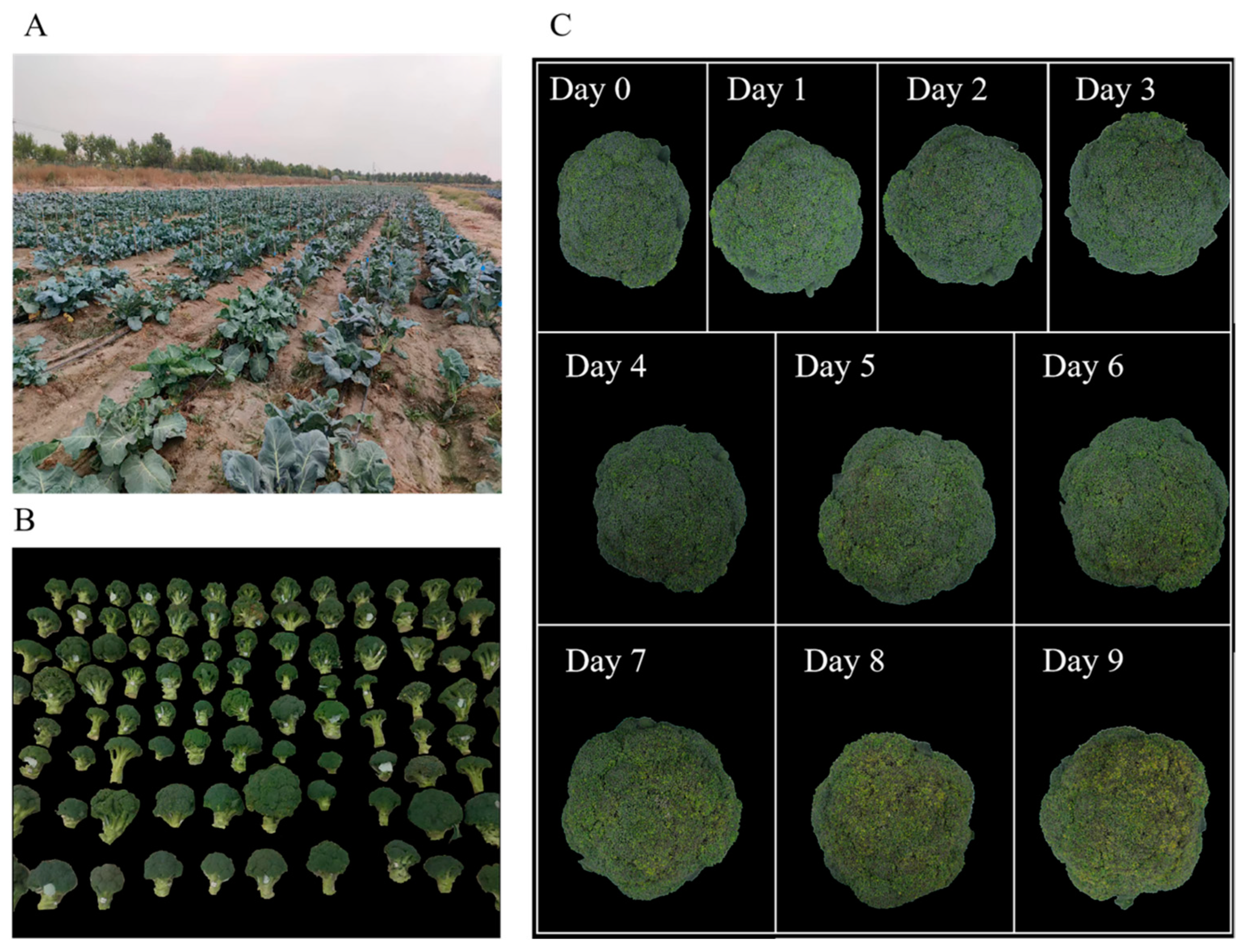
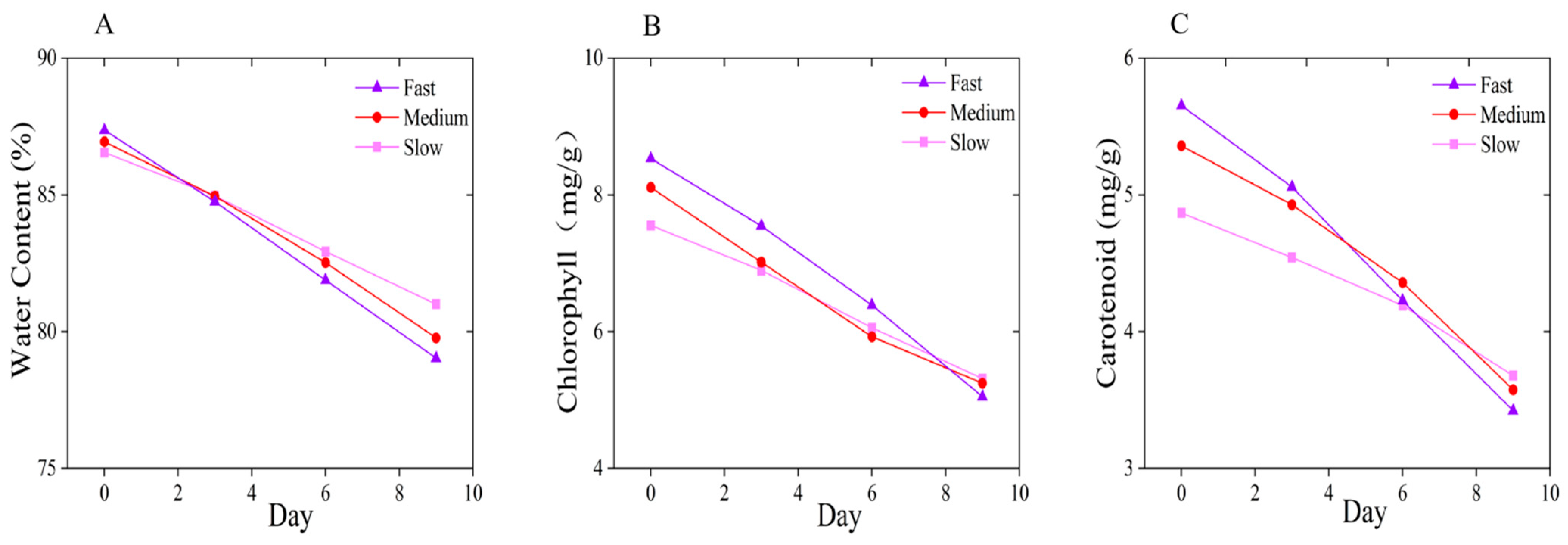
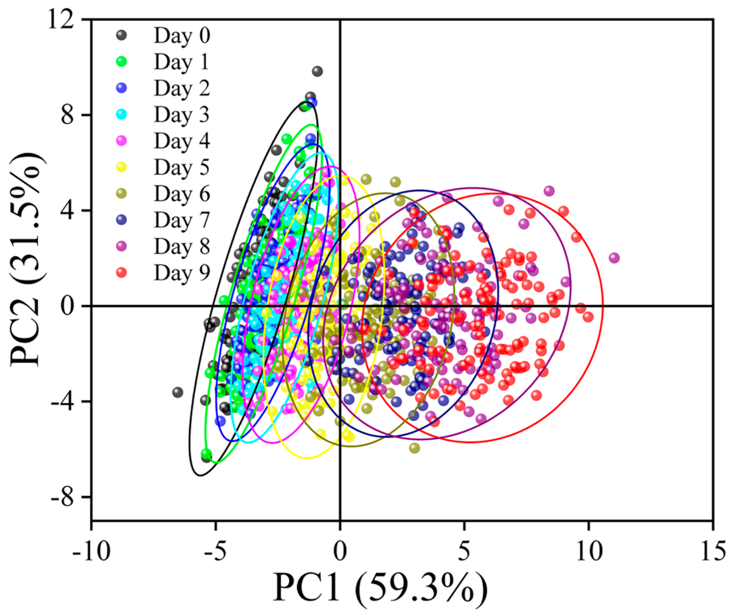
Differences in the color, appearance, and intrinsic substance content of broccoli are present at different shelf life stages. The different colors and wilting degrees of broccoli buds with different shelf lives affect the multispectral image information. In most studies, quality and shelf life are determined only by predicting the intrinsic substance content using spectral technology [35] without considering appearance or texture. However, in this study, the spectral data, textural characteristics, and physical and chemical parameters of broccoli were used to predict and evaluate its shelf life.

Compared to existing traditional methods, this study focuses on the predictive and evaluative performance based on multispectral imaging. Conventional approaches, such as manual evaluation, require extensive expertise, are time-consuming, labor-intensive, and highly subjective, making them difficult to widely apply in practical scenarios [17]. In contrast, this study provides a rapid, non-destructive, and accurate alternative. In contrast to Mohi Alden et al. [36], who manually assessed cauliflower quality based on appearance, odor, and texture during storage, and Joshi et al. 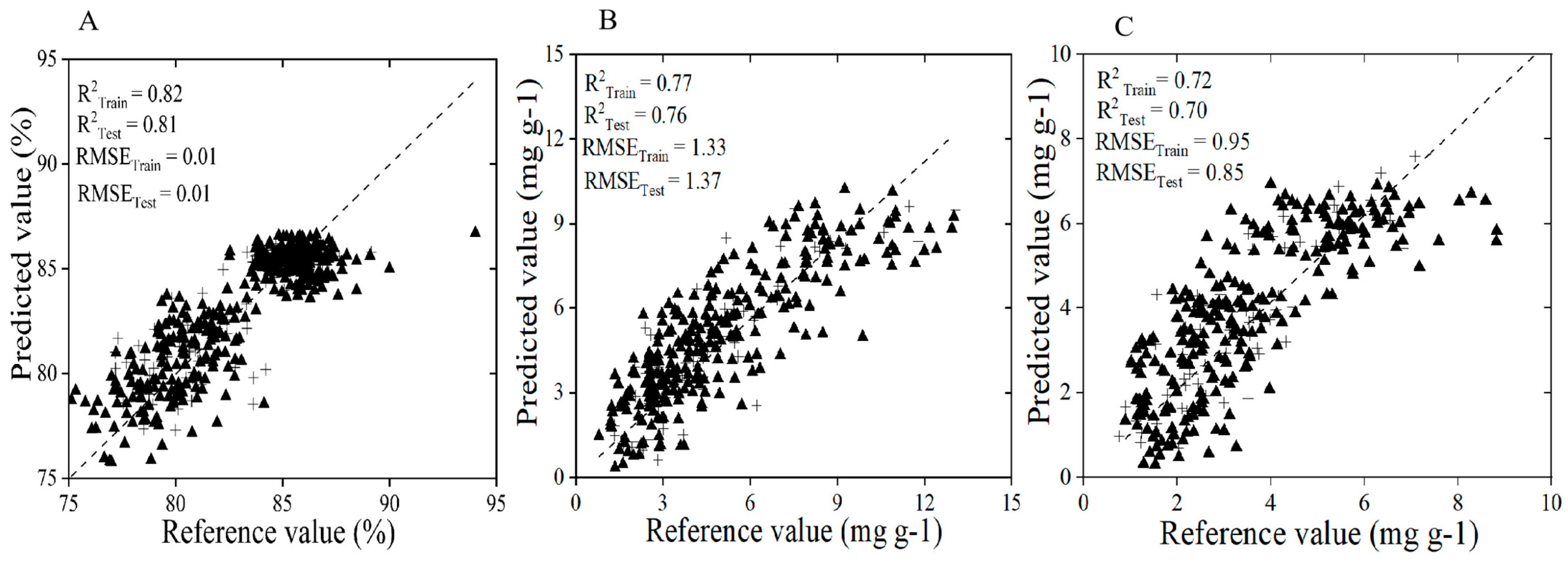[37], who determined strawberry shelf life through sensory evaluation, this study employs multispectral imaging to provide more objective quantitative data, thereby enhancing the accuracy and consistency of the evaluation. The physicochemical parameter prediction model for broccoli shelf life developed in this study enables rapid and non-destructive acquisition of these parameters during practical evaluation. This approach reduces the need for destructive measurements of internal substance content changes in broccoli, significantly improving evaluation efficiency and demonstrating the practical feasibility of the non-destructive method proposed in this research. In this study, the performance of the 2D-CNN model combined with multispectral imaging for predicting physicochemical parameters was significantly lower than that of the SVR and RF models based on one-dimensional spectral data, which is consistent with the findings of Zhang et al. 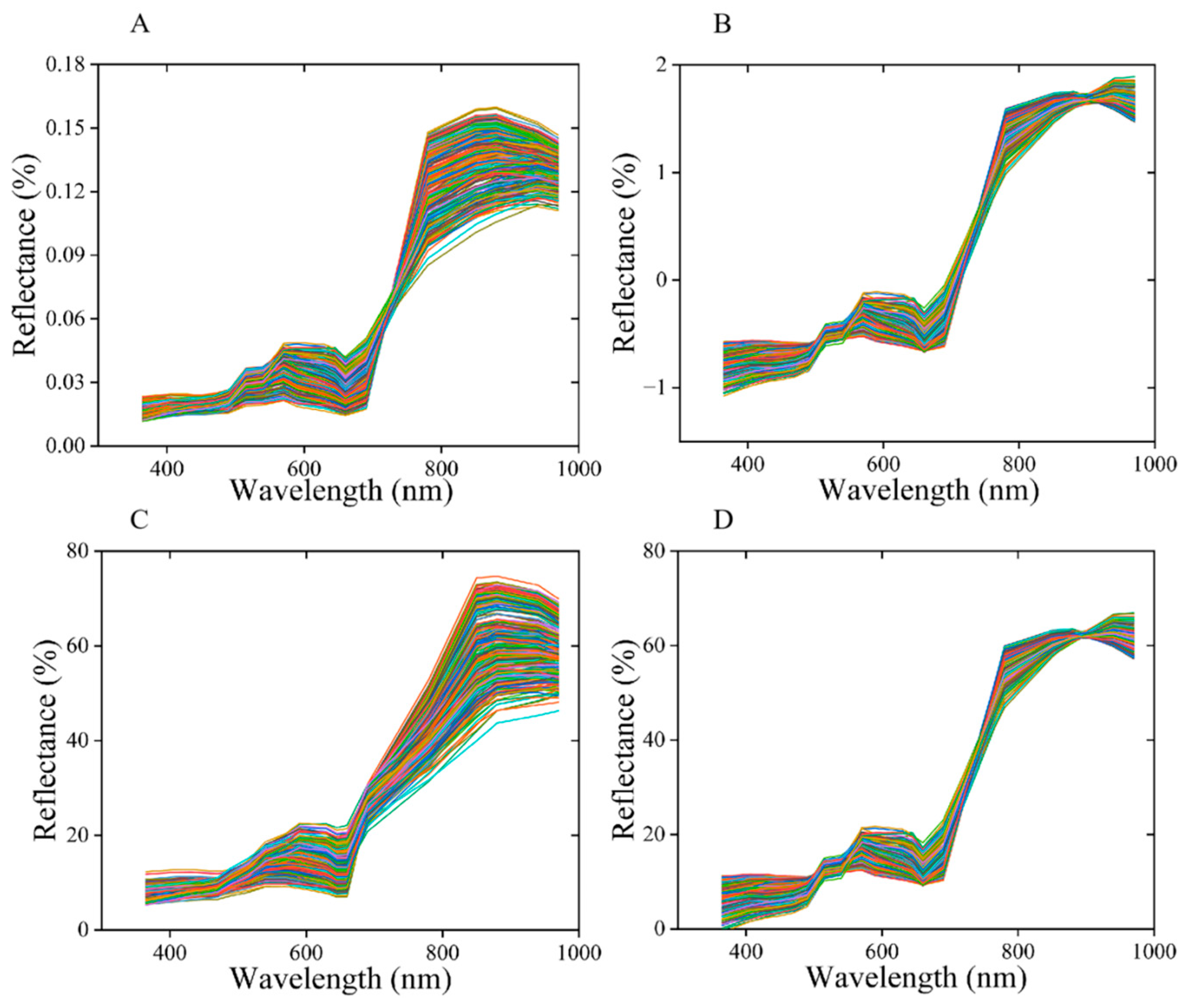[26] in predicting photosynthetic pigments. For the SVR and RF models utilizing one-dimensional spectral data, the SPA algorithm was employed to extract relevant spectral bands, effectively removing irrelevant spectral information and thereby enhancing both the computational efficiency and accuracy of the models. Additionally, four preprocessing methods were applied to the raw spectral data, resulting in improved model accuracy compared to the original data model.

Compared to traditional data fusion methods [38], such as the integration of spectral data and texture features, this study introduces physicochemical parameters, incorporating variations in the internal substance content during broccoli shelf life. This approach further enriches the feature information and enhances the predictive capability of the model, highlighting the advantages of multi-feature fusion. To the best of our knowledge, traditional data fusion methods have primarily been applied to tea grade classification [20] and meat shelf-life assessment [22], with limited application in fruit and vegetable shelf-life evaluation. This study advances the field by further enriching feature information through the incorporation of physicochemical parameters into the existing data fusion framework. In contrast to Rabasco-Vílchez et al. [39], who used near-infrared spectral data to assess strawberry shelf life based on storage time and temperature, this study achieves non-destructive prediction of physicochemical parameters and integrates spectral data, texture features, and physicochemical parameters through multi-feature data fusion for comprehensive broccoli shelf-life evaluation. Compared to Li et al. 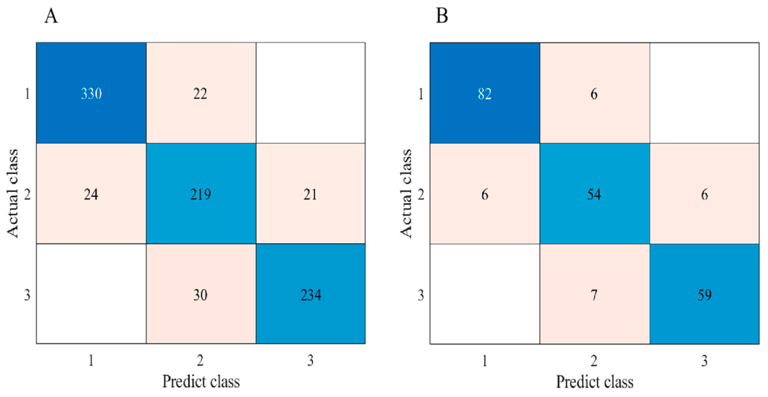[40], who predicted kiwifruit shelf life by assessing substance content using near-infrared spectroscopy, this study further incorporates texture features, capturing both external spatial information and internal substance content, thereby improving evaluation accuracy. This study leverages multi-feature data fusion technology to provide physicochemical parameters reflecting internal substance content and texture features capturing external spatial information, which are crucial for the comprehensive evaluation of appearance changes and internal quality in vegetables such as broccoli. This approach demonstrates superior overall performance. In this study, the SPA+SG+RF model within the RF framework emerged as the best model for broccoli shelf life prediction, achieving training and testing accuracies of 88.98% and 88.64%, respectively. In contrast, the 2D-CNN classification model based on multispectral images showed lower accuracy compared to the 1D-CNN and RF models utilizing multi-feature data fusion. This is because the 2D-CNN model takes 100 × 100 × 19 multispectral images as input without extracting spectral features, and the small gaps and shadows between broccoli florets in the images affect model accuracy. Comparative results from three multi-feature fusion approaches indicate that models combining LBP and GLCM texture features with spectral data outperform those using spectral data alone, while the fusion of spectral data, LBP and GLCM texture features, and physicochemical parameters yields the best performance. This further demonstrates that integrating LBP, GLCM texture features, and physicochemical parameters enhances the accuracy of broccoli shelf-life evaluation and the feasibility of multi-feature data fusion.

Although this study collected a substantial dataset and enriched feature information through multi-feature data fusion, it must be acknowledged that misclassifications still exist, as evidenced by the results of the best classification model (Figure 12). To achieve more accurate broccoli shelf-life evaluation in real-world applications, further optimization of the model structure is necessary to enhance its precision. Additionally, the diversity of the dataset (e.g., variations in growing environments and storage conditions) remains relatively limited, which may constrain the model’s generalizability in diverse retail or supply chain scenarios. Future research could expand the dataset to include broccoli samples from different growing environments and storage conditions, explore additional types of spectral image data and physicochemical parameters, and further refine data fusion methods to improve model generalizability. Meanwhile, with the continuous advancement of artificial intelligence and deep learning technologies, more sophisticated neural network models are expected to provide even more precise shelf life prediction and evaluation. Furthermore, this research could be extended to the shelf-life assessment of other vegetables and fruits, offering theoretical support and practical guidance for advancements in food preservation technology.

5. Conclusions

The objective of this study is to explore the application of multispectral imaging technology combined with multi-feature data fusion for the prediction and evaluation of broccoli shelf life. The SPA+SG+RF model, utilizing multi-feature fusion data type C for broccoli shelf-life assessment, achieved training and testing accuracies of 88.98% and 88.64%, respectively. Based on the current findings, the integration of multispectral imaging technology, multi-feature data fusion, and machine learning can serve as an effective method for predicting and evaluating broccoli shelf life. This approach enables managers to assess broccoli shelf life efficiently, rapidly, and non-destructively, offering a novel pathway for the development of online prediction and evaluation systems for broccoli shelf life.

References

1. Li, H.; Xia, Y.; Liu, H.-Y.; Guo, H.; He, X.-Q.; Liu, Y.; Wu, D.-T.; Mai, Y.-H.; Li, H.-B.; Zou, L.; et al. Nutritional values, beneficial effects, and food applications of broccoli (Brassica oleracea var. italica Plenck). Trends Food Sci. Technol. 2022, 119, 288–308. [Google Scholar] [CrossRef]
2. Zhang, X.; Yang, Q.; Luo, M.; Song, M.; Zhou, Q.; Chen, J.; Ji, S. Insights into profiling of p-coumaric acid treatment on delaying the yellowing of broccoli. Postharvest Biol. Technol. 2023, 201, 112371. [Google Scholar] [CrossRef]
3. Pintos, F.M.; Hasperué, J.H.; Vicente, A.R.; Rodoni, L.M. Role of white light intensity and photoperiod during retail in broccoli shelf-life. Postharvest Biol. Technol. 2020, 163, 111121. [Google Scholar] [CrossRef]
4. Shi, J.; Gao, L.; Zuo, J.; Wang, Q.; Wang, Q.; Fan, L. Exogenous sodium nitroprusside treatment of broccoli florets extends shelf life, enhances antioxidant enzyme activity, and inhibits chlorophyll-degradation. Postharvest Biol. Technol. 2016, 116, 98–104. [Google Scholar] [CrossRef]
5. Patil, M.; Sharma, S.; Sridhar, K.; Anurag, R.K.; Grover, K.; Dharni, K.; Mahajan, S.; Sharma, M. Effect of postharvest treatments and storage temperature on the physiological, nutritional, and shelf-life of broccoli (Brassica oleracea) microgreens. Sci. Hortic. 2024, 327, 112805. [Google Scholar] [CrossRef]
6. Paulsen, E.; Barrios, S.; Baenas, N.; Moreno, D.A.; Heinzen, H.; Lema, P. Effect of temperature on glucosinolate content and shelf life of ready-to-eat broccoli florets packaged in passive modified atmosphere. Postharvest Biol. Technol. 2018, 138, 125–133. [Google Scholar] [CrossRef]
7. Zhan, L.; Hu, J.; Li, Y.; Pang, L. Combination of light exposure and low temperature in preserving quality and extending shelf-life of fresh-cut broccoli (Brassica oleracea L.). Postharvest Biol. Technol. 2012, 72, 76–81. [Google Scholar] [CrossRef]
8. Pintos, F.; Rodoni, L.; Patrignani, M.; Ixtaina, P.; Vicente, A.; Martínez, G.; Hasperué, J. Advances in the use of white light on broccoli and kale postharvest shelf life. Innov. Food Sci. Emerg. Technol. 2023, 86, 103373. [Google Scholar] [CrossRef]
9. Loi, M.; Liuzzi, V.C.; Fanelli, F.; De Leonardis, S.; Maria Creanza, T.; Ancona, N.; Paciolla, C.; Mulè, G. Effect of different light-emitting diode (LED) irradiation on the shelf life and phytonutrient content of broccoli (Brassica oleracea L. var italica). Food Chem. 2019, 283, 206–214. [Google Scholar] [CrossRef]
10. Xu, D.; Zuo, J.; Fang, Y.; Yan, Z.; Shi, J.; Gao, L.; Wang, Q.; Jiang, A. Effect of folic acid on the postharvest physiology of broccoli during storage. Food Chem. 2021, 339, 127981. [Google Scholar] [CrossRef]
11. Cai, J.-H.; Luo, F.; Zhao, Y.-B.; Zhou, Q.; Wei, B.-D.; Zhou, X.; Ji, S.-J. 24-Epibrassinolide treatment regulates broccoli yellowing during shelf life. Postharvest Biol. Technol. 2019, 154, 87–95. [Google Scholar] [CrossRef]
12. Jiang, X.; Tian, J.; Huang, H.; Hu, X.; Han, L.; Huang, D.; Luo, H. Nondestructive visualization and quantification of total acid and reducing sugar contents in fermented grains by combining spectral and color data through hyperspectral imaging. Food Chem. 2022, 386, 132779. [Google Scholar] [CrossRef] [PubMed]
13. Sharma, S.; Sirisomboon, P.; Sumesh, K.C.; Terdwongworakul, A.; Phetpan, K.; Kshetri, T.B.; Sangwanangkul, P. Near-infrared hyperspectral imaging combined with machine learning for physicochemical-based quality evaluation of durian pulp. Postharvest Biol. Technol. 2023, 200, 112334. [Google Scholar] [CrossRef]
14. Zahra, A.; Qureshi, R.; Sajjad, M.; Sadak, F.; Nawaz, M.; Khan, H.A.; Uzair, M. Current advances in imaging spectroscopy and its state-of-the-art applications. Expert Syst. Appl. 2024, 238, 122172. [Google Scholar] [CrossRef]
15. Sricharoonratana, M.; Thompson, A.K.; Teerachaichayut, S. Use of near infrared hyperspectral imaging as a nondestructive method of determining and classifying shelf life of cakes. LWT 2021, 136, 110369. [Google Scholar] [CrossRef]
16. Siripatrawan, U.; Makino, Y. Simultaneous assessment of various quality attributes and shelf life of packaged bratwurst using hyperspectral imaging. Meat Sci. 2018, 146, 26–33. [Google Scholar] [CrossRef] [PubMed]
17. Shao, Y.; Ji, S.; Xuan, G.; Wang, K.; Xu, L.; Shao, J. Soluble solids content monitoring and shelf life analysis of winter jujube at different maturity stages by Vis-NIR hyperspectral imaging. Postharvest Biol. Technol. 2024, 210, 112773. [Google Scholar] [CrossRef]
18. Tang, Y.; Wang, F.; Zhao, X.; Yang, G.; Xu, B.; Zhang, Y.; Xu, Z.; Yang, H.; Yan, L.; Li, L. A nondestructive method for determination of green tea quality by hyperspectral imaging. J. Food Compos. Anal. 2023, 123, 105621. [Google Scholar] [CrossRef]
19. Hu, Y.; Huang, P.; Wang, Y.; Sun, J.; Wu, Y.; Kang, Z. Determination of Tibetan tea quality by hyperspectral imaging technology and multivariate analysis. J. Food Compos. Anal. 2023, 117, 105136. [Google Scholar] [CrossRef]
20. Yin, Y.; Li, J.; Ling, C.; Zhang, S.; Liu, C.; Sun, X.; Wu, J. Fusing spectral and image information for characterization of black tea grade based on hyperspectral technology. LWT 2023, 185, 115150. [Google Scholar] [CrossRef]
21. Zhang, H.; Zhang, S.; Chen, Y.; Luo, W.; Huang, Y.; Tao, D.; Zhan, B.; Liu, X. Non-destructive determination of fat and moisture contents in Salmon (Salmo salar) fillets using near-infrared hyperspectral imaging coupled with spectral and textural features. J. Food Compos. Anal. 2020, 92, 103567. [Google Scholar] [CrossRef]
22. Lytou, A.; Fengou, L.-C.; Koukourikos, A.; Karampiperis, P.; Zervas, P.; Carstensen, A.S.; Del Genio, A.; Carstensen, J.M.; Schultz, N.; Chorianopoulos, N.; et al. Seabream quality monitoring throughout the supply chain using a portable multispectral imaging device. J. Food Prot. 2024, 87, 100274. [Google Scholar] [CrossRef] [PubMed]
23. Zhang, S.; Duan, X.; Yan, X.; Yuan, X.; Zhang, D.; Liu, Y.; Wang, Y.; Shen, S.; Xuan, S.; Zhao, J.; et al. Multispectral detection of dietary fiber content in Chinese cabbage leaves across different growth periods. Food Chem. 2024, 447, 138895. [Google Scholar] [CrossRef]
24. Yang, S.; Jia, Z.; Yi, K.; Zhang, S.; Zeng, H.; Qiao, Y.; Mao, P.; Li, M. Rapid prediction and visualization of safe moisture content in alfalfa seeds based on multispectral imaging technology. Ind. Crop. Prod. 2024, 222, 119448. [Google Scholar] [CrossRef]
25. Duan, Z.; Li, H.; Li, C.; Zhang, J.; Zhang, D.; Fan, X.; Chen, X. A CNN model for early detection of pepper Phytophthora blight using multispectral imaging, integrating spectral and textural information. Plant Methods 2024, 20, 1–12. [Google Scholar] [CrossRef]
26. Zhang, J.; Zhang, D.; Cai, Z.; Wang, L.; Wang, J.; Sun, L.; Fan, X.; Shen, S.; Zhao, J. Spectral technology and multispectral imaging for estimating the photosynthetic pigments and SPAD of the Chinese cabbage based on machine learning. Comput. Electron. Agric. 2022, 195, 106814. [Google Scholar] [CrossRef]
27. Zhang, D.; Zhang, J.; Peng, B.; Wu, T.; Jiao, Z.; Lu, Y.; Li, G.; Fan, X.; Shen, S.; Gu, A.; et al. Hyperspectral model based on genetic algorithm and SA-1DCNN for predicting Chinese cabbage chlorophyll content. Sci. Hortic. 2023, 321, 112334. [Google Scholar] [CrossRef]
28. Mishra, P.; Sadeh, R.; Bino, E.; Polder, G.; Boer, M.P.; Rutledge, D.N.; Herrmann, I. Complementary chemometrics and deep learning for semantic segmentation of tall and wide visible and near-infrared spectral images of plants. Comput. Electron. Agric. 2021, 186, 106226. [Google Scholar] [CrossRef]
29. Agustika, D.K.; Mercuriani, I.; Purnomo, C.W.; Hartono, S.; Triyana, K.; Iliescu, D.D.; Leeson, M.S. Fourier transform infrared spectrum pre-processing technique selection for detecting PYLCV-infected chilli plants. Spectrochim. Acta Part A Mol. Biomol. Spectrosc. 2022, 278, 121339. [Google Scholar] [CrossRef]
30. Azadnia, R.; Rajabipour, A.; Jamshidi, B.; Omid, M. New approach for rapid estimation of leaf nitrogen, phosphorus, and potassium contents in apple-trees using Vis/NIR spectroscopy based on wavelength selection coupled with machine learning. Comput. Electron. Agric. 2023, 207, 107746. [Google Scholar] [CrossRef]
31. Singha, C.; Swain, K.C.; Sahoo, S.; Govind, A. Prediction of soil nutrients through PLSR and SVMR models by VIs-NIR reflectance spectroscopy. Egypt. J. Remote. Sens. Space Sci. 2023, 26, 901–918. [Google Scholar] [CrossRef]
32. Barea-Sepúlveda, M.; Ferreiro-González, M.; Calle, J.L.P.; Barbero, G.F.; Ayuso, J.; Palma, M. Comparison of different processing approaches by SVM and RF on HS-MS eNose and NIR Spectrometry data for the discrimination of gasoline samples. Microchem. J. 2022, 172, 106893. [Google Scholar] [CrossRef]
33. Khodabakhshian, R.; Emadi, B.; Khojastehpour, M.; Golzarian, M.R. Determining quality and maturity of pomegranates using multispectral imaging. J. Saudi Soc. Agric. Sci. 2017, 16, 322–331. [Google Scholar] [CrossRef]
34. Zhou, C.; Hu, J.; Xu, Z.; Yue, J.; Ye, H.; Yang, G. A monitoring system for the Segmentation and grading of broccoli head based on deep learning and neural networks. Front. Plant Sci. 2020, 11, 402. [Google Scholar] [CrossRef]
35. Benelli, A.; Cevoli, C.; Fabbri, A.; Ragni, L. Ripeness evaluation of kiwifruit by hyperspectral imaging. Biosyst. Eng. 2022, 223, 42–52. [Google Scholar] [CrossRef]
36. Mohi Alden, K.; Omid, M.; Rajabipour, A.; Tajeddin, B.; Soltani Firouz, M. Quality and shelf-life prediction of cauliflower under modified atmosphere packaging by using artificial neural networks and image processing. Comput. Electron. Agric. 2019, 163, 104861. [Google Scholar] [CrossRef]
37. Joshi, P.; Pahariya, P.; Al-Ani, M.F.; Choudhary, R. Monitoring and prediction of sensory shelf-life in strawberry with ultraviolet-visible-near-infrared (UV-VIS-NIR) spectroscopy. Appl. Food Res. 2022, 2, 100123. [Google Scholar] [CrossRef]
38. Xie, Z.; Yan, J.; Liang, H.; Yue, X.; Su, X.; Wei, H.; Lu, Y.; Fan, X.; Ma, W.; Zhang, X.; et al. PLS-DA model for accurate identification of Chinese cabbage leaf color based on multispectral imaging. Veg. Res. 2023, 3, 25. [Google Scholar] [CrossRef]
39. Rabasco-Vílchez, L.; Jiménez-Jiménez, F.; Possas, A.; Brunner, M.; Fleck, C.; Pérez-Rodríguez, F. Evaluating the shelf life of strawberries using a portable Vis-NIR spectrophotometer and a Reflectance Quality Index (RQI). Postharvest Biol. Technol. 2024, 218, 113189. [Google Scholar] [CrossRef]
40. Li, H.; Zhu, L.; Li, N.; Liu, Z.; Wang, L.; Chitrakar, B.; Xu, D.; Cui, Z.; Tang, Y.; Hu, L.; et al. NIR spectroscopy for quality assessment and shelf-life prediction of kiwifruit. Postharvest Biol. Technol. 2024, 218, 113201. [Google Scholar] [CrossRef]
Figure 1. Experimental materials. (A): Broccoli planting site. (B): Broccoli experimental samples. (C): Broccoli samples collected daily.
Agronomy 15 00788 g001
Figure 2. Overall research workflow. SG: Savitzky Golay convolution smoothing algorithm, SNV: standard normal variate algorithm, NOR: normalization algorithm, MSC: multiplicative scatter correction algorithm, SPA: successive projection algorithm, SVR: support vector regression algorithm, RF: random forest algorithm, and CNN: convolutional neural network algorithm.
Agronomy 15 00788 g002
Figure 3. Structure of the two-dimensional convolutional neural network (2D-CNN) regression model. The left half of the figure depicts the composition of the convolutional modules, while the right half illustrates the entire process of predicting physicochemical parameters using convolutional modules, fully connected layers, and regression layers with 19-channel spectral images as input. Conv_Layer: convolutional layer; Leaky ReLU Layer: leaky rectified linear unit layer.
Agronomy 15 00788 g003
Figure 4. Structure of the one-dimensional convolutional neural network (1D-CNN) classification model, illustrating the entire process from the input layer to the output of the classification layer. Conv_Layer: convolutional layer; ReLU Layer: rectified linear unit layer.
Agronomy 15 00788 g004
Figure 5. Structure of the two-dimensional convolutional neural network (2D-CNN) classification model. The left half of the figure depicts the composition of the convolutional modules, while the right half illustrates the entire process of classification using the convolutional module, fully connected layer, loss function layer, and classification layer with 19-channel spectral images as input. Conv_Layer: convolutional layer; Leaky ReLU Layer = leaky rectified linear unit layer.
Agronomy 15 00788 g005
Figure 6. Changes in physicochemical parameter contents in broccoli during shelf life. (A): change in water content, (B): change in chlorophyll content, and (C): change in carotenoid content.
Agronomy 15 00788 g006
Figure 7. (A): original spectral curve; (B): daily average spectral curve.
Agronomy 15 00788 g007
Figure 8. Spectral curves of raw spectra after different preprocessing methods. (A): normalized spectral curve, (B): standard normal variate (SNV) spectral curve, (C): Savitzky–Golay (SG) spectral curve, and (D): multiplicative scatter correction (MSC) spectral curve.
Agronomy 15 00788 g008
Figure 9. Principal component analysis (PCA) plot of raw spectral data.
Agronomy 15 00788 g009
Figure 10. Fitting graphs of the best prediction models for physicochemical parameters. The best prediction model fitting graphs for (A) water content, (B) chlorophyll, and (C) carotenoid. Triangles: training set; crosses: validation set.
Agronomy 15 00788 g010
Figure 11. Extraction of spectral data relevant feature bands using the successive projection algorithm (SPA). Relevant feature bands of spectral data after (A) Savitzky Golay convolutional smoothing, (B) standard normal variate transformation, and (C) normalization preprocessing.
Agronomy 15 00788 g011
Figure 12. Results of the best model discriminant. (A): confusion matrix for the training set, (B): confusion matrix for the validation set. The numbers 1, 2, and 3 in the figure represent the three grades for broccoli shelf life classification.
Agronomy 15 00788 g012