Effects of Long-Term Input of Controlled-Release Urea on Maize Growth Monitored by UAV-RGB Imaging

Abstract

Maize is a critical crop for global food security, yet excessive nitrogen (N) application, while sustaining yields, leads to reduced nitrogen use efficiency (NUE), and the application of controlled-release fertilizer (CRF) is one of the effective options to achieve sustainable maize production while improving NUE. This study evaluated the long-term effects of CRF with varying N input rates on maize growth using low-cost UAV-RGB imaging. UAV-RGB images were captured in different growth stages, and the non-canopy background was removed using the maximum between-class algorithm (OTSU). Eleven vegetation indices were constructed from the images to analyze maize growth under different N treatments. The results indicated that a single application of CRF with an equivalent N input rate to conventional treatment yielded significantly better outcomes. The optimal controlled-release N ratio was 40% of the total N input, increasing maize yield by 6.73% and NUE by 15%. Indices such as NRI, NBI, ARVI, RGBVI, ExR, ExG, and ExGR effectively reflected plant N status, with R² values exceeding 0.856 for yield estimation across growth stages. UAV-RGB imaging proved to be a viable method for rapid N status monitoring, aiding in the optimization of N management in maize production.

1. Introduction

Maize is the cereal crop with the widest planting range and the largest yield in the world today, ranking first among the major grains [1]. Nitrogen (N) is an important component of structural molecules such as chlorophyll, nucleic acid, and protein in maize plants, which can not only regulate the growth of maize but also affect the final maize yield and protein content [2]. The timing and optimal amount of nitrogen application constitute critical strategies for effective nitrogen management in practice [3]. Due to the difficulty in topdressing in the middle and later periods of dryland maize production, it is difficult to use the N fertilizer applied by topdressing to coordinate the relationship between the maize N demand and soil N supply during the filling period, which can easily cause N deficiency, lowering the filling rate and N use efficiency (NUE). N deficiency in the late growth period causes premature leaf senescence, resulting in reduced yield, and the contribution rate of nitrogen fertilizer in the process of increasing crop yield exceeds 40% [4]. However, in practice, the overdose application of N will not contribute to a significant increase in maize yield, but will instead reduce NUE, resulting in maize quality reduction, soil erosion, and environmental pollution [5]. Controlled-release fertilizer (CRF) realizes the backward action of N nutrients by slowing down and controlling the dissolution and release rate of nutrients. It can increase the photosynthetic characteristics of maize chlorophyll content in the jointing period, increase the grain filling rate, reduce the apparent loss of N in the field when compared to the traditional N fertilizer application method, significantly increasing NUE, and ultimately increase grain yield [6,7]. The use of CRF can not only reduce the cost of topdressing but also provide the N demand for the early growth of maize, promote the formation of organ morphology and dry matter accumulation, and at the same time solve the problem of N deficiency when the maximum accumulation rate of dry matter occurs in the middle period before grain filling [8,9].

The application of CRF is one of the keys to high-yielding maize for stable production, and N is a crucial factor that influences the growth, quality, and the ultimate yield of maize; thus, controlling nitrogen levels within an appropriate range is a prerequisite and assurance for efficient planting [10,11]. Presently, Kjeldahl’s method is a commonly used laboratory method for detecting nitrogen content in crops [12]. However, this method requires field sampling and the subsequent transportation of samples to the laboratory for nitrogen measurement, making it time-consuming, labor-intensive and less efficient, and unsuitable for large-scale testing. As a result, the timely and precise monitoring and evaluation of nitrogen levels during maize growth are of significant importance for improving nitrogen utilization efficiency and maize yield.

Chemical methods, which are time- and cost-consuming, are conventionally used in the characterization of the long-term effect of CRF input. In recent years, remote sensing technology has provided an alternative option for precise fertilization and N nutrition diagnosis, and remote sensing can quickly and non-destructively obtain the spectral information of crops [13,14]. In the past few decades, satellite remote sensing technology has been widely used to predict crop N content in different geographic locations and scales for nutrient assessment [15]. However, satellite remote sensing showed limitations such as low spatiotemporal resolution and was easily restricted by meteorological conditions [16,17], making it unsuitable for crop N assessment on small and medium regional scales. The development of unmanned aerial vehicle (UAV) remote sensing technology promoted the high-precision acquisition of small- and medium-scale agricultural planting information, and it has been used in crop N nutrition diagnosis, growth monitoring, yield estimation, disaster assessment, agricultural production management decision making, etc. [18,19,20,21]. Changes in soil N supply can affect the amount of chlorophyll in leaves, altering the spectral characteristics of the maize canopy as it grows [22]. The N content of crops during this time was reflected in the color depth and spectral reflectance properties of crop canopy pixels [23]. Nowadays, multi-spectral and hyperspectral images are mostly used in UAV remote sensing, and a good performance of the vegetation index created using multi-spectral UAV red-edge and near-infrared bands for monitoring wheat leaf N content and estimating protein content was achieved [24,25,26]. Although low-cost and easy-to-obtain UAV RGB color images have been increasingly used in the field of crop planting information extraction [27,28], the investigations were mainly based on short-term experiments, with long-term effects remaining unclear.

In this study, a long-term experiment of CRF input on maize production was used for monitoring using UAV-RGB images, and the main objectives of this study were to (1) select the vegetation index for effectively monitoring N status in maize growth, and build an effective model for yield estimation; and (2) explore the long-term effects of CRF on maize production, and optimize N management for CRF application.

2. Materials and Methods

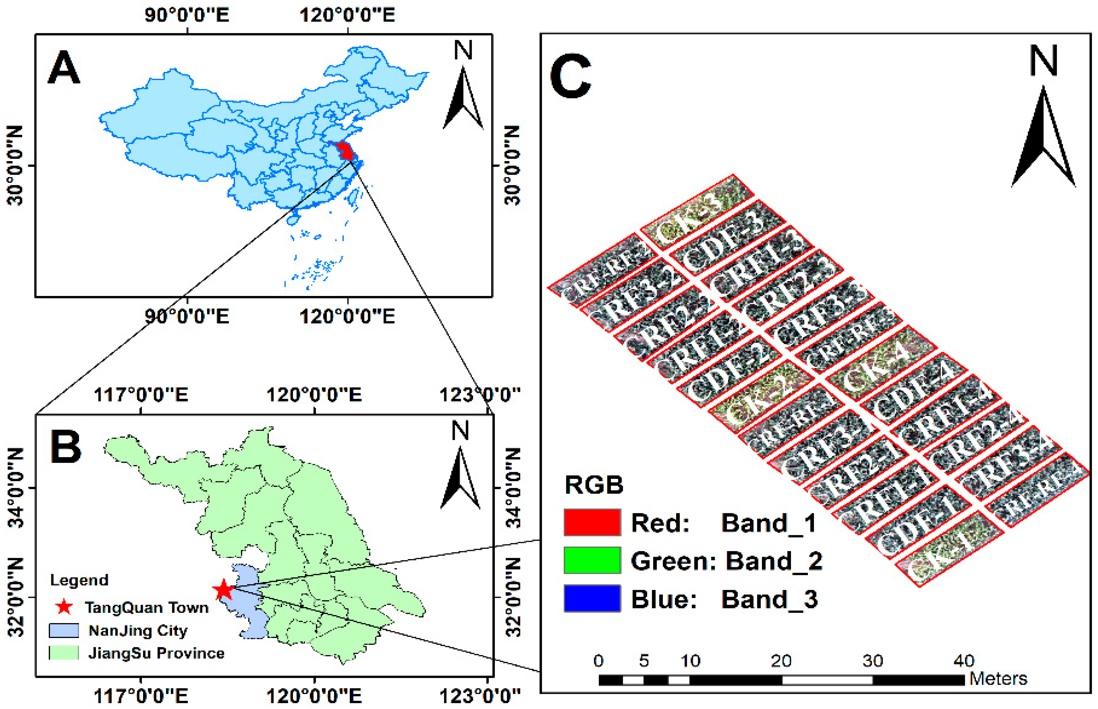
2.1. Study Area

The long-term CRF experiment in this study was started in 2012, which was located in Tangquan Town, Pukou District, Nanjing City, Jiangsu Province (118°27′ E, 32°05′ N), with an average annual temperature of around 15–16 °C. Annual precipitation is approximately 1000–1100 mm concentrated from June to August. The predominant soil type is paddy soil (yellow-brown soil), characterized by relatively high organic matter content (1.5–2.5%), a pH range of 5.5–6.5, and good water retention capacity. The used CRF was provided by Jiangsu ISSAS New Fertilizer Engineering & Technology Co., Ltd. (Yangzhou, China). The CRF was coated with waterborne polyacrylate at a rate of 8%, the N content was 41.7%, and the N release longevity was 3 months. The experimental site and plot design are shown in Figure 1. There were 6 different N treatments, each treatment contained 4 replicates, and each plot had an area of 40 m² (4 m × 10 m).

Six N fertilizer treatments were set with different N input rates (

Table 1. Fertilization treatments.

Treatment	Fertilization Method	N (kg ha−1)	P2O5 (kg ha−1)	K2O (kg ha−1)	CRN Ratio (%)
CK	No fertilization	-	-	-	-
CDF	Conventional fertilizer, twice-split	240	60	135	0
CRF1	Controlled-release fertilizer, one application	240	60	135	30
CRF2	Controlled-release fertilizer, one application	240	60	135	40
CRF3	Controlled-release fertilizer, one application	240	60	135	50
CRF-RF	Controlled-release fertilizer, one application, 15% N reduced	204	60	135	50

). In conventional fertilizer treatment (CDF), half of the N fertilizer was the base fertilizer, and the others were topdressed in the earing stage. In the CRF1, CRF2, CRF3, and CRF-RF treatments, all N was fertilized as base fertilizers. In the CRF1 treatment, controlled-release N (CRN) accounts for 30% of total N input, 40% in the CRF2 treatment, and 50% in the CRF3 and CRF-RF treatments. The CRF-RF was treated with reduced N input as well as straw returning. The yield of each treatment was measured during harvesting. The maize variety used was Suyu 29, the sowing time was mid-May 2019, and the harvest time was the end of September 2019.

2.2. Data Collection

The average yields of each treatment in 2019 are summarized as follows (Figure 2): CK, 4454.4 kg ha⁻¹; CDF, 8117.5 kg ha⁻¹; CRF1, 8531.9 kg ha⁻¹; CRF2, 8703.1 kg ha⁻¹; CRF3, 8604.4 kg ha⁻¹; and CRF-RF, 8689.4 kg ha⁻¹. The average yields of each treatment in 2020 are summarized as follows: CK, 1402.5 kg ha⁻¹; CDF, 7289.7 kg ha⁻¹; CRF1, 7715.6 kg ha⁻¹; CRF2, 7452.5 kg ha⁻¹; CRF3, 7310.3 kg ha⁻¹; and CRF-RF, 6308.8 kg ha⁻¹.

Throughout the critical growth stages of maize (

Table 2. The time of UAV image collection.

Date of Data Collection	Growth Period
14 July 2019	Trileaf period
26 July 2019	Jointing period
12 August 2019	Tasseling period
27 August 2019	Silking period
8 September 2019	Pustulation period

), RGB imagery was acquired by employing a DJI Phantom 4 Pro unmanned aerial system (UAS), specifically equipped with a 20-megapixel visible-light (RGB) lens. The high-resolution RGB images were captured within defined wavelength intervals: the red (R) band spanned the spectral range of 450 ± 16 nm, the green (G) band covered 560 ± 16 nm, and the blue (B) band encompassed 650 ± 16 nm.

The sampling time was between 10:00 and 14:00, and the camera could automatically focus, expose, and adjust the white balance. Each flight was carried out under clear, cloudless, and windless conditions. The side overlap rate and course overlap were both set to 75%, and the flight altitude was set as 150 m. Images were taken according to the fixed route in each experiment in the DJI Terra v3.3.4 (Shenzhen DJI Technology Co., Ltd., Shenzhen, China), the UAV-RGB image was imported into the software, geometric correction was performed, a dense point cloud was constructed, and high-definition orthoimages were generated in tiff format with geographic coordinates (Figure 3).

2.3. Image Preprocessing

2.3.1. UAV Image Data Information Extraction and Index Construction

Vegetation indices, serving as remote sensing indicators for farmland health monitoring, have become a core tool in modern digital agricultural management. By integrating meteorological and soil data, they enable the dynamic tracking of crop growth and yield prediction. These indices can rapidly respond to disaster events, precisely identify affected areas to support insurance damage assessment, and generate high-resolution vegetation index maps to facilitate precision management of water and fertilizer application. Plant leaves showed strong absorption in the visible-light range due to the presence of pigments, especially chlorophyll a and b. This adsorption creates two valleys in the blue and red regions and a reflection peak in the green region, which could be used to identify and quantify vegetation. The image indices are mathematical operations applied to the digital number values of different bands, which provided useful information about plant health, growth, and nutrient content. Since N is one of the main components of chlorophyll, the content of chlorophyll is directly closely related to N abundance. According to the sensors carried by the UAV remote sensing platform used, 11 commonly used visible-light remote sensing vegetation indices were selected in this study (

Table 3. Vegetation indices used in this study.

Name	Index	Formulation	References
Normalized Red light Index	NRI	$NRI={\displaystyle \frac{R}{R+G+B}}$	/
Normalized Green light Index	NGI	$NGI={\displaystyle \frac{G}{R+G+B}}$	/
Normalized Blue light Index	NBI	$NBI={\displaystyle \frac{B}{R+G+B}}$	/
Green Leaf Index	GLI	$GLI={\displaystyle \frac{2G-R-B}{2R+G+B}}$	[29]
Green Red Vegetation Index	GRVI	$GRVI={\displaystyle \frac{G-R}{G+R}}$	[30]
Atmospherically Resistant Vegetation Index	ARVI	$ARVI={\displaystyle \frac{G-R}{G+R-B}}$	[31]
Modified Green Red Vegetation Index	MGRVI	$MGRVI={\displaystyle \frac{G^2-R^2}{G^2+R^2}}$	[32]
Red–Green–Blue Vegetation Index	RGBVI	$RGBVI={\displaystyle \frac{G^2-RB}{g^2-rb}}$	[33]
Excess Red Index	ExR	$ExR=1.4R-G$	[34]
Excess Green Index	ExG	$ExG=2G-R-B$	[34]
Excess Green minus Excess Red Index	ExGR	$ExGR=3G-2.4R-B$	[35]

Note: R, G, and B of the RGB image denote the normalized values of the three bands.

). The RGB sensor captures only three spectral bands: red (600–700 nm), green (500–600 nm), and blue (400–500 nm). Different vegetation indices capture the differential responses of plant physiological parameters through mathematical combinations of specific spectral bands. The Normalized Red-Edge Index (NRI) and Nitrogen Band Index (NBI), based on the absorption sensitivity of red-edge bands to the chlorophyll-nitrogen complex, directly reflect the metabolic levels of chloroplast nitrogen. The Atmospherically Resistant Vegetation Index (ARVI) introduces blue band correction for atmospheric scattering, providing a more stable characterization of canopy photosynthetic active radiation interception efficiency. The Red–Green–Blue Vegetation Index (RGBVI) and the ExG/ExR/ExGR series focus on combinatorial relationships within visible bands (red, green, blue), where the Excess Green Index (ExG) enhances the response to chlorophyll reflectance peaks and shows sensitivity to nitrogen allocation during leaf expansion. The Excess Green minus Red (ExGR) index specifically captures nitrogen remobilization during leaf senescence by differentially eliminating soil background interference. These physiological distinctions among indices originate from their target parameters: NRI/NBI emphasizes nitrogen–photosystem associations, ARVI prioritizes canopy light-use efficiency, and RGB-based indices reflect structural nitrogen allocation during leaf development stages. Selection criteria should therefore integrate the target crop’s nitrogen metabolism characteristics (e.g., nitrogen remobilization during reproductive growth versus nitrogen accumulation in vegetative phases) and the scale-dependent physiological processes (canopy-level responses versus single-leaf level changes) under observation.

To extract the corresponding values of different vegetation indexes from the remote sensing images in each plot, ArcGIS 10.8 (ESRI, Redlands, CA, USA) was used to perform band operations on the images to obtain the index results. Then, the “Output statistical results in tables” was used to generate statistics on each plot, and the average value of each index was used as the index value for each plot.

2.3.2. OTSU Method

The OTSU algorithm, also known as the maximum inter-class variance method, is a commonly used algorithm in threshold segmentation that can automatically generate optimal segmentation thresholds for images [36]. This method relies on global thresholds and exhibits weak robustness against uneven illumination or local contrast variations (such as shadows and reflections). Therefore, when acquiring remote sensing images during different periods, it is essential to select the same weather conditions and time frames whenever possible. The basic principle assumes that image I(x, y) can be divided into background and foreground regions based on threshold T. Here, the proportion of foreground pixels in the entire image is denoted as w₀, with their average gray value recorded as μ₀; the proportion of background pixels is denoted as w₁, with their average gray value as μ₁. The total average gray value of the entire image is denoted as μ, and the inter-class variance is denoted as g. The algorithm can ultimately be simplified to the following formula:

$$g=w_0{w}_1{({\mu }_0-{\mu }_1)}^2$$

(1)

The OTSU threshold segmentation was implemented in MATLAB software (version 2018a, MathWorks, Inc. Natick, MA, USA). The canopy coverage of each plot was different, which resulted in the image containing pixels of two types of ground objects, maize and soil. To reduce the influence of the non-canopy part, the OTSU threshold segmentation method was used to process the G channel in the RGB image.

2.4. Data Analysis

2.4.1. ReliefF Feature Weight Selection

When dealing with a large number of feature parameters, selecting high-contribution features and discarding low-contribution features could improve the accuracy of classification or regression. ReliefF, a filter-based feature selection method, could measure the importance of each feature using relevant statistical metrics. The basic idea was to evaluate each feature variable by selecting a random sample R from the sample set during each iteration, and choose k nearest neighbor samples from the same and different classes of R to update the weights of each feature. The number of nearest neighbors k could affect the weight values of the feature variables. It is important to determine a stable k value to select features; for small-sample datasets, k can be set to a smaller value [37], and k was set as 4 in this study.

2.4.2. Variance Expansion Factor

The variance inflation factor (VIF) was used to measure the severity of multicollinearity among variables in a multiple linear regression model, which represented the correlation between explanatory variables, and it was defined as

$$VIF={\displaystyle \frac{1}{1-R_i^2}}$$

(2)

where R²_i represents the coefficient of determination between the i-th variable and other variables. In general, when 0 ≤ VIF < 10, there is no multicollinearity in the regression model; when 10 ≤ VIF ≤ 20, the regression model shows certain multicollinearity; and when VIF > 20, the regression model indicates serious multicollinearity.

2.4.3. Linear Regression Modeling

The multiple linear regression model was used to describe the relationship between the dependent variable Y changes and the change in multiple independent variables X (Equation (3)):

$$\mathrm{Y}={\beta }_0+{\beta }_1{x}_1+{\beta }_2{x}_2+\cdots +{\beta }_n{x}_n$$

(3)

where Y is the yield; β₀ is a constant term; β₁, β₂, ⋯, β_n are regression coefficients; and x₁, x₂, ⋯, x_n are constructed vegetation indices. Through the model, the best yield estimation equation for each growth period was obtained.

2.5. Model Evaluation

For evaluating the prediction performance of models, the coefficient of determination (R²) and the root-mean-square error (RMSE) were used (Equations (4) and (5)).

$$R^2=1-{\displaystyle \frac{{{\sum }_{i=1}^n(y-\widehat{y})}^2}{{{\sum }_{i=1}^n(y-\overline{y})}^2}}$$

(4)

$$RMSE=\sqrt{{\displaystyle \frac{{\sum }_{i=1}^n{(y-\widehat{y})}^2}{n}}}$$

(5)

where y represents the measured yield, $\widehat{y}$ represents the simulated yield, $\overline{y}$ represents the mean yield, and n represents the number of samples.

3. Results

3.1. OTSU Threshold Segmentation

The optimal segmentation thresholds for the G channel of remote sensing images during the different growth stages are 94 for the trileaf period, 93 for the jointing period, 86 for the tasseling period, 86 for the silking period, and 102 for the pustulation period. Figure 4 illustrates the final segmentation results, and it was observed that there was much soil background in the original UAV-RGB image (Figure 4a₂), but after threshold segmentation processing, an image with an obviously removed soil background was obtained, as shown in Figure 4b₂. Through threshold segmentation processing, the crown and soil elements were well distinguished, reducing the impact of non-crown parts on the accuracy of image information extraction.

3.2. Vegetation Indices Constructed Under Different Fertilization Conditions and Growth Periods

To better explain the change in vegetation indices, the indices constructed by extracting the canopy image in each growth period under different fertilization conditions was averaged (Figure 5). Since CK was not fertilized, there were large differences with other treatments in whole growth periods. As CDF was fertilized twice, it could be clearly observed that the indices changed greatly after the fertilizer application. However, the indices of CDF became closer to the other treatments after the spinning period. The remaining four treatments, using CRF, could continuously release nutrients during the growth period of maize, reducing nutrient loss and improving nutrient utilization efficiency, thereby minimizing nutrient waste and providing a sustained nutrient supply for corn. Therefore, from the three-leaf period to the jointing period, except for ARVI, MGRVI, and RGBVI, all other index values showed improvement, consistent with visual observations of the original images. From the tasseling period to the filling period, the leaf color of the canopy on the original image changed greatly. In these periods, except for the NGI and ExR indices, the values of all other indices gradually decreased.

3.3. Correlation Analysis of Yield and Indices in Different Growth Periods

3.3.1. Weight Selection of ReliefF Features

Table 4. ReliefF weight selection for each vegetation index in different growth periods.

Index	Trileaf Period	Jointing Period	Tasseling Period	Silking Period	Pustulation Period
NRI	0.0003	0.1469	0.1935	0.2762	0.1832
NGI	0.1538	0.1936	0.2034	0.3351	0.2473
NBI	0.0772	0.0203	0.0891	0.3354	0.0376
GRVI	0.0004	0.0203	0.1929	0.2663	0.1834
GLI	0.0968	0.0363	0.1223	0.2951	0.0500
ARVI	0.0797	0.1473	0.0891	0.2723	0.0376
MGRVI	0.0006	0.1505	0.1871	0.2662	0.1962
RGBVI	0.0766	0.0220	0.1033	0.3221	0.0873
ExR	0.0003	0.1469	0.1935	0.2646	0.1832
ExG	0.0314	0.1093	0.0839	0.3351	0.0695
ExGR	0.2366	0.2366	0.2366	0.3512	0.2366

shows ReliefF weights for vegetation indices under six different fertilization treatments. The best result was obtained with the n value set to 4. Five index values with the highest weight in each growth period were selected, among which ExGR, NGI, GLI, ARVI, and NBI were selected in the three-leaf period; ExGR, NGI, MGRVI, NRI, and ARVI in the jointing period; ExGR in the tasseling period; NGI, NRI, ExR, RGBVI, ExGR, NBI, ExG, NGI, and RGBVI in the silking period; and NGI, ExGR, MGRVI, GRVI, and ExR in the grouting period.

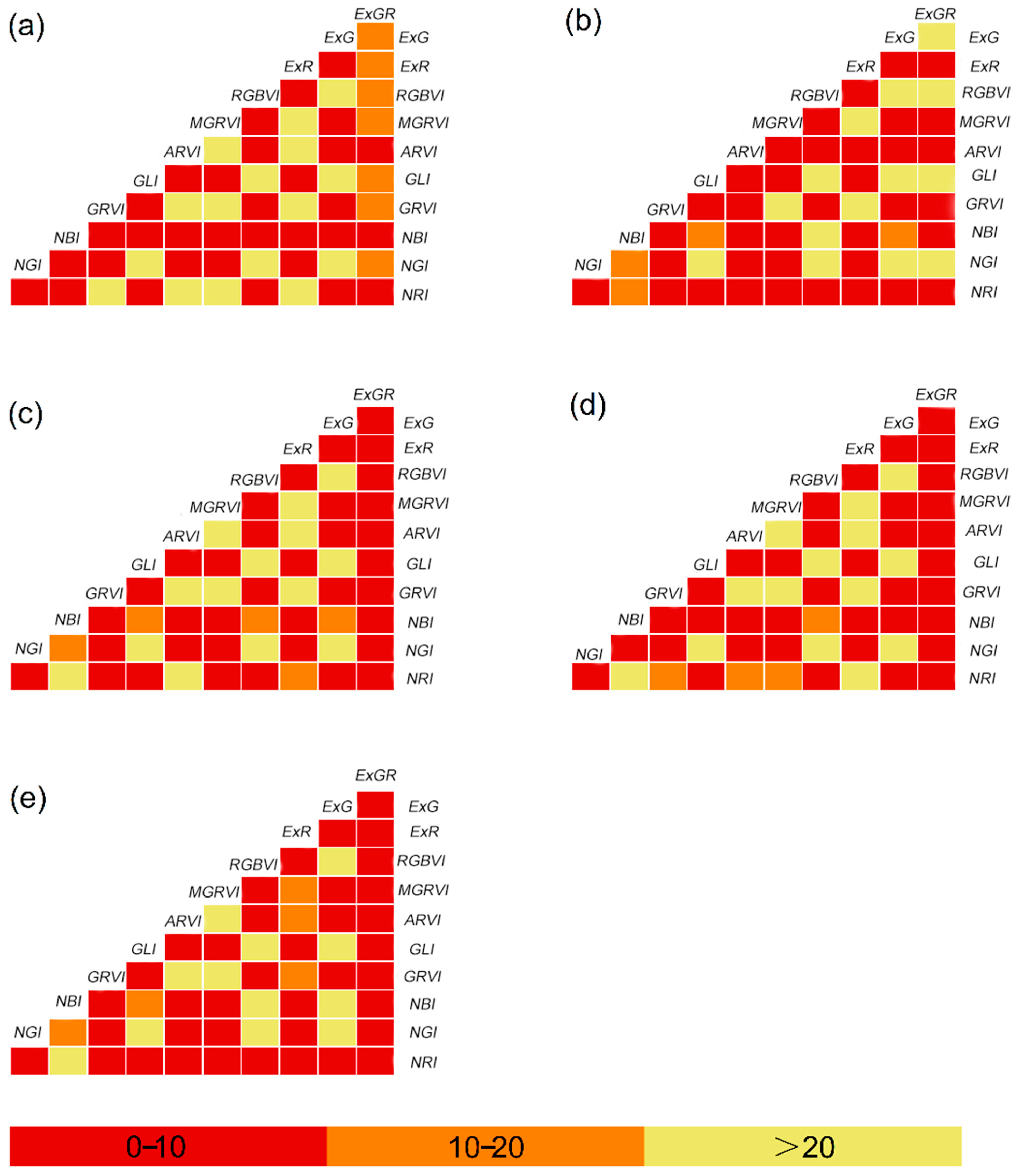
3.3.2. Construct Collinearity Analysis Between Vegetation Indices

The method of VIF was used to conduct multicollinearity analysis among the constructed vegetation indices (Figure 6).

When 0 ≤ VIF < 10, there is no multicollinearity between the image indices; when 10 ≤ VIF < 20, there is a certain collinearity between the image indices; and when VIF ≥ 20, there is serious collinearity between the image indices. According to the definition of collinearity, priority was given to indices with a higher number of VIF values ≤ 10 relative to other indices, and 5 indices with lower collinearity were selected for each growth period. NBI, GLI, ARVI, RGBVI, and ExG were selected in the three-leaf period; NRI, GRVI, ARVI, and MGRVI were selected in the jointing period; ExR, NRI, GRVI, MGRVI, RGBVI, and ExGR were selected in the tasseling period; NGI, NBI, GLI, ExG, and ExGR were selected in the silking period; and NRI, ARVI, MGRVI, ExR, and ExGR were selected in the pustulation period.

3.3.3. Correlation Analysis

Under different fertilization conditions, the canopy image construction index extracted in each growth period was correlated with the final yield (

Table 5. The correlation coefficient between the index constructed under each growth period and the yield.

Index	Trileaf Period	Jointing Period	Tasseling Period	Silking Period	Pustulation Period
NRI	−0.842 **	−0.858 **	−0.890 **	−0.920 **	−0.918 **
NGI	0.328	−0.922 **	−0.909 **	−0.879 **	−0.905 **
NBI	0.850 **	0.943 **	0.931 **	0.944 **	0.940 **
GRVI	0.736 **	−0.065	0.690 **	0.798 **	0.584 **
GLI	0.331	−0.922 **	−0.907 **	−0.878 **	−0.904 **
ARVI	0.786 **	0.607 **	0.794 **	0.819 **	0.643 **
MGRVI	0.736 **	−0.063	0.691 **	0.798 **	0.584 **
RGBVI	0.330	−0.926 **	−0.908 **	−0.904 **	−0.915 **
ExR	−0.744 **	−0.015	−0.773 **	−0.852 **	−0.676 **
ExG	0.328	−0.922 **	−0.940 **	−0.882 **	−0.906 **
ExGR	0.564 **	−0.861 **	−0.698 **	−0.216	−0.715 **

Note: ** Correlation is significant at 0.01 level (two-tailed).

). There was a significant correlation (p < 0.01) between most of the canopy vegetation indices constructed under the trileaf period and jointing period and the final yield. There was a significant negative correlation among them, while there was a significant positive correlation between NBI, GRVI, ARVI, MGRVI, and ExGR and the yield, among which the index with the most significant negative correlation was NRI with a value of −0.842, and the index with the most significant positive correlation was NBI, with a value of 0.850. In the jointing period, there were extremely significant positive correlations between NBI and ARVI and the yield, while there were extremely significant negative correlations between NRI, NGI, GLI, RGBVI, ExG, and ExGR and the yield, respectively. The index with the largest significant positive correlation was NBI with a value of 0.943, and the index with the largest extremely significant negative correlation was RGBVI with a value of −0.926. In the tasseling period, silking period, and pustulation period, however, there was a significant correlation in almost all of them. Under the three growth periods, the four indices of NBI, GRVI, ARVI, and MGRVI were all extremely and positively correlated in a statistically significant manner. Except for ExGR under the silking period, the indices were extremely and negatively correlated under each growth period in a statistically significant manner. The indices with the most significant positive correlations under the three growth periods were NBI, with values of 0.931, 0.944, and 0.940 in the tasseling period, silking period, and pustulation period, respectively. The indices with the most extreme significant negative correlations were ExG, NRI, and NRI with values of −0.940, −0.920, and −0.918, respectively.

For effectively expressing the change in N content under different treatments, effectively reducing the multicollinearity in the model, and ensuring the image index is sensitive to the final yield inversion, the VIF feature screening results and correlation coefficient were integrated. The vegetation indices with weak collinearity and strong correlation were selected for modeling. Combined with Table 4 and Table 5 and Figure 6, the coincidence indices were selected as multivariate variables for multiple linear regression modeling under different growth periods. Therefore, NBI and ARVI were selected in the trileaf period; NRI and ARVI were selected in the jointing period; NRI, ExGR, and RGBVI were selected in the tasseling period; NBI and ExG were selected in the silking period; and ExR and ExGR were selected in the pustulation period.

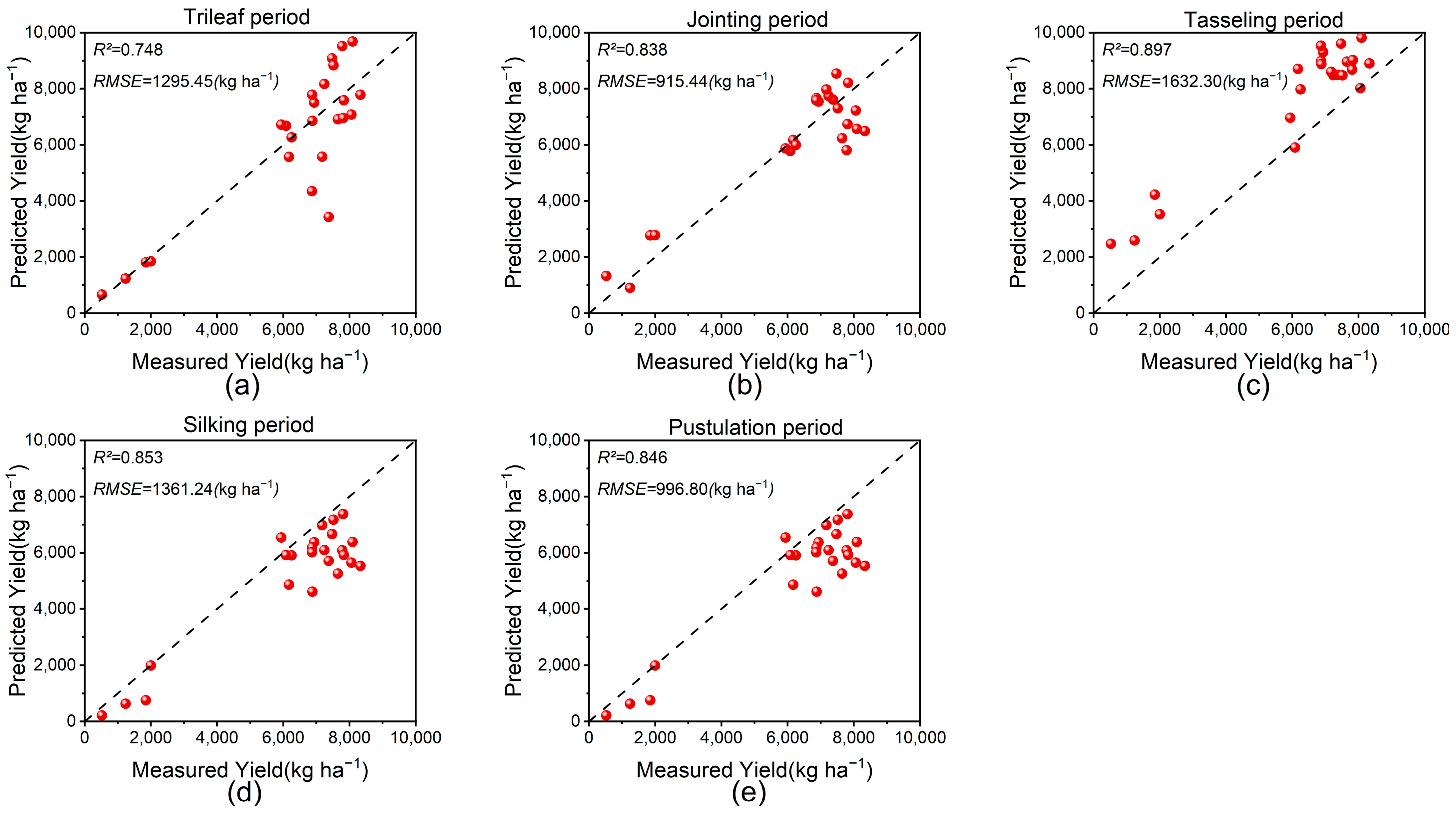
3.4. Optimum Yield Estimation Model for Each Growth Period Using Linear Regression

According to the ReliefF feature screening results and correlation coefficient, the vegetation index that was more sensitive to the final yield in each growth period was selected, the dataset was randomly divided into training and validation sets in a 3:1 ratio, and the yield estimation inversion model for each growth period was established through linear regression (

Table 6. Regression model of optimal yield estimation in each growth period.

Maize Growth Period	Equation of Regression
Trileaf period	$Y=\mathrm{12,143.1}NBI+\mathrm{108,457.5}ARVI-\mathrm{28,854.7}$
Jointing period	$Y=-\mathrm{376,561.4}NRI-\mathrm{90,300.7}ARVI+\mathrm{143,946.8}$
Tasseling period	$Y=-\mathrm{487,586.6}NRI-\mathrm{297,113.8}ExGR+\mathrm{249,280.1}RGBVI+\mathrm{132,835.3}$
Silking period	$Y=\mathrm{88,970.182}NBI-\mathrm{13,334.226}ExG-\mathrm{17,707.877}$
Pustulation period	$Y=-\mathrm{86,140.8}ExGR-\mathrm{185,319.5}ExR+\mathrm{25,520.8}$

).

The models in each growth period were validated. The R² of the validation set in the trileaf period was 0.856, and the RMSE was 626.03 (kg ha⁻¹). The R² of the validation set in the jointing period was 0.906, and the RMSE was 590.47 (kg ha⁻¹). The R² of the validation set in the tasseling period was 0.894, and the RMSE was 536.70 (kg ha⁻¹). The R² of the validation set in the silking period was 0.897, and the RMSE was 516.33 (kg ha⁻¹). The R² of the validation set in the pustulation period was 0.910, and the RMSE was 533.20 (kg ha⁻¹).

4. Discussion

4.1. Optimum Vegetation Index for Growth Monitoring in Different Growth Periods

The nitrogen nutritional status of crops is closely related to canopy color. Remote sensing RGB image detection, with its advantages of high resolution, high efficiency, and non-destructive characteristics, could broadly reflect maize growth conditions, thereby compensating for the shortcomings of traditional laboratory testing methods. Vegetation indices such as NRI, NBI, ARVI, RGBVI, ExG, ExR, and ExGR, screened based on the variance inflation coefficient and correlation coefficient, could effectively characterize maize growth conditions in different developmental stages. These indices have been widely applied in crop growth monitoring [38]. The effectiveness of different indices across various growth stages under CRF input conditions is summarized in

Table 7. The specific performance of the selected vegetation indices across different growth periods under CRF input.

Vegetation Index	Applicable Growth Period	Specific Expressions	Relationship with the Literature	References
NRI NBI	All growth periods	Real-time maize growth monitoring throughout lifecycle	This study revealed the dynamic responses of plant canopy images to CRF input.	/
ARVI	Trileaf period Jointing period	Superior performance was demonstrated comparied with the traditional NDVI under specific atmospheric conditions.	ARVI considered the atmospheric disturbance, and this study validated its applicability under specific climatic conditions	[39]
RGBVI ExG ExR ExGR	Jointing period Tasseling period Silking period Pustulation period	Vegetation coverage was reflected by improved monitoring effectiveness under CRF input	These VIs expanded the description of the long-term effects of CRF input on maize regarding promoting maize growth	[33,34,35]

.

The values of these indices showed similar trends in different growth periods. During the trileaf period and jointing period, the values of CDF were higher than those of CRF1, CRF2, CRF3, and CRF-RF, as CDF was directly applied as the nitrogen fertilizer that took immediate effect after application. After entering the tasseling period, several growth periods were characterized by vigorous vegetative and reproductive growth of maize, which was also the critical period for determining maize yield formation. CRF started to release nutrients and promoted maize growth, causing the vegetation index values of CRF1, CRF2, CRF3, and CRF-RF to gradually increase and surpass those of CDF, resulting in different final yields. The values of these vegetation indices were correlated with the final yield to a certain extent, indicating their effectiveness in nitrogen diagnosis.

4.2. The Best Yield Estimation Model for Each Growth Period

According to the established yield estimation models for different growth stages, the optimal indices used for monitoring maize growth and yield estimation might not necessarily be the same for different periods, which could be attributed to environmental and meteorological factors during the collection of UAV images. In addition to the R² values of 0.856 for the model predicted in the three-leaf stage and 0.860 for the model predicted in the jointing stage, most of the models built for other growth stages achieved R² values above 0.907. The observed and predicted values of the models were mostly distributed around the 1:1 line, indicating good accuracy and reliability of these models (Figure 7). This phenomenon might be caused by the fact that before the jointing stage, the maize leaves were not very large, resulting in more exposed bare ground, which might have a certain impact on the spectral information collected by the UAV and thus lowered the accuracy of the model. However, during the tasseling, silking, and grain filling stages, the maize leaves were large, resulting in greater ground coverage and less exposed bare ground, thus reducing the impact on the spectral information collected by the UAV.

Validation using UAV visible-light image data from different growth stages in 2020 yielded good results when the extracted indices were plugged into the constructed prediction equations for different growth stages. Similarly, as maize growth progresses, the results obtained from prediction equations for later growth stages were better than those obtained from the three-leaf stage, with an R² value of 0.748 for the model predicted in the three-leaf stage, and R² values above 0.838 for models predicted in other growth stages. However, the RMSE of the results obtained from the five yield estimation equations was higher than that of the results from 2019, which might be due to differences in data collection dates and years, leading to acceptable changes in spectral information and resulting in certain errors in the model predictions.

4.3. Optimal Nutrient Management Model

Among the six treatments in this experiment, CRF2 had the highest average yield, followed by CRF-RF, CRF3, CRF1, CDF, and CK. When comparing the effects of different proportions of controlled-release nitrogen fertilizers (CRFs) in CDF, CRF1, CRF2, and CRF3, with all other conditions held constant, it was evident that the application of CRF resulted in a better yield compared to the direct application of nitrogen fertilizers. The treatment with a CRF proportion of 40% achieved the highest yield increase of 6.73%. When comparing CRF3 and CRF-RF, both treatments had a CRF proportion of 50%, but CRF-RF reduced nitrogen fertilizer application by 15% and increased the yield by approximately 0.98%. The difference in yield per hectare between CRF-RF and CRF2 was not significant. Considering cost and environmental pollution factors, CRF-RF was identified as the best nutrient management strategy in this experiment. Based on the vegetation indices extracted from remote sensing, NRI and ExR values gradually increased during the maize growth period, while NGI, GRVI, GLI, ARVI, MGRVI, RGBVI, ExGR, and ExG values decreased gradually, showing a certain regularity. The changes in vegetation indices were most pronounced from the jointing period to the silking period. This phenomenon might be attributed to the nutrient’s controlled release from CRF after the jointing period, thus promoting rapid maize growth [40,41], which indicated that monitoring nutrient changes using UAV-RGB images was feasible.

5. Conclusions

UAV-RGB remote sensing data collected during various growth stages of maize can be utilized to construct vegetation indices, with non-canopy pixels effectively removed using the OTSU algorithm. Subsequently, optimal vegetation indices for each growth stage were identified through ReliefF feature selection, variance inflation factor (VIF) analysis, and correlation coefficients. These indices were then used to establish yield estimation models. The indices NRI, NBI, ARVI, RGBVI, ExR, ExG, and ExGR demonstrated the ability to effectively reflect the growth status of maize across different growth stages. The low-cost RGB UAV-derived yield estimation models for critical growth stages demonstrated high accuracy and reliability. Specifically, the application of controlled-release nitrogen at a 40% proportion of total nitrogen input (CRF2) increased yield by 6.73%, while a 15% reduction in nitrogen input with a 50% proportion of controlled-release nitrogen (CRF-RF) also resulted in a yield increase. Therefore, vegetation indices derived from UAV-RGB images confirmed that both CRF2 and CRF-RF treatments are recommended for maize cultivation in this region, offering a balance between economic (yield) and environmental (NUE) benefits. This approach provides a viable alternative for optimizing nutrient management in maize production. In future, we can advance UAV RGB remote sensing imaging from ‘phenomenon monitoring’ to ‘intelligent decision-making assessment’ by integrating with other sensors and conducting long-term positioning observations, which will provide technical support for the optimization of CRF input in sustainable crop production.

References

1. IFAD; UNICEF. The State of Food Security and Nutrition in the World 2017; FAO: Rome, Italy, 2017. [Google Scholar]
2. Chen, X.; Cui, Z.; Fan, M.; Vitousek, P.; Zhao, M.; Ma, W.; Wang, Z.; Zhang, W.; Yan, X.; Yang, J. Producing more grain with lower environmental costs. Nature 2014, 514, 486–489. [Google Scholar] [CrossRef] [PubMed]
3. Ahmad, I.; Batyrbek, M.; Ikram, K.; Ahmad, S.; Kamran, M.; Misbah; Khan, R.S.; Hou, F.; Han, Q. Nitrogen management improves lodging resistance and production in maize (Zea mays L.) at a high plant density. J. Integr. Agric. 2023, 22, 417–433. [Google Scholar] [CrossRef]
4. Elisante, E.; Muzuka, A. Occurrence of nitrate in Tanzanian groundwater aquifers: A review. Appl. Water Sci. 2015, 7, 71–87. [Google Scholar] [CrossRef]
5. Du, L.; Zhao, T.; Zhang, C.; An, Z.; Wu, Q.; Liu, B.; Li, P.; Ma, M. Investigations on nitrate pollution of soil, groundwater and vegetable from three typical farmlands in Beijing region, China. Agric. Sci. China 2011, 10, 423–430. [Google Scholar] [CrossRef]
6. Ke, J.; He, R.; Hou, P.; Ding, C.; Ding, Y.; Wang, S.; Liu, Z.; Tang, S.; Ding, C.; Chen, L.; et al. Combined controlled-released nitrogen fertilizers and deep placement effects of N leaching, rice yield and N recovery in machine-transplanted rice. Agric. Ecosyst. Environ. 2018, 265, 402–412. [Google Scholar] [CrossRef]
7. Xiao, Y.; Peng, F.; Zhang, Y.; Wang, J.; Zhuge, Y.; Zhang, S.; Gao, H. Effect of bag-controlled release fertilizer on nitrogen loss, greenhouse gas emissions, and nitrogen applied amount in peach production. J. Clean. Prod. 2019, 234, 258–274. [Google Scholar] [CrossRef]
8. Yao, Z.; Zhang, W.; Wang, X.; Zhang, L.; Zhang, W.; Liu, D.; Chen, X. Agronomic, environmental, and ecosystem economic benefits of controlled-release nitrogen fertilizers for maize production in Southwest China. J. Clean. Prod. 2021, 312, 127611. [Google Scholar] [CrossRef]
9. Ji, P.; Peng, Y.; Cui, Y.; Li, X.; Tao, P.; Zhang, Y. Effects of reducing and postponing controlled-release urea application on soil nitrogen regulation and maize grain yield. Int. J. Agric. Biol. Eng. 2022, 15, 116–123. [Google Scholar] [CrossRef]
10. Nyiraneza, J.; N’Dayegamiye, A.; Chantigny, M.H.; Laverdière, M.R. Variations in corn yield and nitrogen uptake in relation to soil attributes and nitrogen availability indices. Soil Sci. Soc. Am. J. 2009, 73, 317–327. [Google Scholar] [CrossRef]
11. Meng, Q.; Hou, P.; Wu, L.; Chen, X.; Cui, Z.; Zhang, F. Understanding production potentials and yield gaps in intensive maize production in China. Field Crop. Res. 2013, 143, 91–97. [Google Scholar] [CrossRef]
12. Miphokasap, P.; Honda, K.; Vaiphasa, C.; Souris, M.; Nagai, M. Estimating canopy nitrogen concentration in sugarcane using field imaging spectroscopy. Remote Sens. 2012, 4, 1651–1670. [Google Scholar] [CrossRef]
13. Qiu, Z.; Xiang, H.; Ma, F.; Du, C. Qualifications of rice growth indicators optimized at different growth stages using unmanned aerial vehicle digital imagery. Remote Sens. 2020, 12, 3228. [Google Scholar] [CrossRef]
14. Wang, R.; Bowling, L.; Cherkauer, K. Estimation of the effects of climate variability on crop yield in the Midwest USA. Agric. For. Meteorol. 2016, 216, 141–156. [Google Scholar] [CrossRef]
15. Battude, M.; Al Bitar, A.; Morin, D.; Cros, J.; Huc, M.; Marais Sicre, C.; Le Dantec, V.; Demarez, V. Estimating maize biomass and yield over large areas using high spatial and temporal resolution Sentinel-2 like remote sensing data. Remote Sens. Environ. 2016, 184, 668–681. [Google Scholar] [CrossRef]
16. Berni, J.; Zarco-Tejada, P.; Suarez, L.; Fereres, E. Thermal and narrowband multispectral remote sensing for vegetation monitoring from an unmanned aerial vehicle. IEEE Trans. Geosci. Remote Sens. 2009, 47, 722–738. [Google Scholar] [CrossRef]
17. Yu, N.; Li, L.; Schmitz, N.; Tian, L.F.; Greenberg, J.A.; Diers, B.W. Development of methods to improve soybean yield estimation and predict plant maturity with an unmanned aerial vehicle based platform. Remote Sens. Environ. 2016, 187, 91–101. [Google Scholar] [CrossRef]
18. Jeong, S.; Ko, J.; Kim, M.; Kim, J. Construction of an unmanned aerial vehicle remote sensing system for crop monitoring. J. Appl. Remote Sens. 2016, 10, 026027. [Google Scholar] [CrossRef]
19. Li, B.; Xu, X.; Zhang, L.; Han, J.; Bian, C.; Li, G.; Liu, J.; Jin, L. Above-ground biomass estimation and yield prediction in potato by using UAV-based RGB and hyperspectral imaging. ISPRS J. Photogramm. Remote Sens. 2020, 162, 161–172. [Google Scholar] [CrossRef]
20. Do-Duy, T.; Nguyen, L.D.; Duong, T.Q.; Khosravirad, S.R.; Claussen, H. Joint optimisation of real-time deployment and resource allocation for UAV-aided disaster emergency communications. IEEE J. Sel. Areas Commun. 2021, 39, 3411–3424. [Google Scholar] [CrossRef]
21. Huang, Y.; Thomson, S.J.; Hoffmann, W.C.; Lan, Y.; Fritz, B.K. Development and prospect of unmanned aerial vehicle technologies for agricultural production management. Int. J. Agric. Biol. Eng. 2013, 6, 1–10. [Google Scholar] [CrossRef]
22. Shi, J.; Wang, Y.; Li, Z.; Huang, X.; Shen, T.; Zou, X. Simultaneous and nondestructive diagnostics of nitrogen/magnesium/potassium-deficient cucumber leaf based on chlorophyll density distribution features. Biosyst. Eng. 2021, 212, 458–467. [Google Scholar] [CrossRef]
23. Bendig, J.; Bolten, A.; Bennertz, S.; Broscheit, J.; Eichfuss, S.; Bareth, G. Estimating biomass of barley using crop surface models (CSMs) derived from UAV-based RGB imaging. Remote Sens. 2014, 6, 10395–10412. [Google Scholar] [CrossRef]
24. Fu, Z.; Yu, S.; Zhang, J.; Xi, H.; Gao, Y.; Lu, R.; Zheng, H.; Zhu, Y.; Cao, W.; Liu, X. Combining UAV multispectral imagery and ecological factors to estimate leaf nitrogen and grain protein content of wheat. Eur. J. Agron. 2022, 132, 126405. [Google Scholar] [CrossRef]
25. Astaoui, G.; Dadaiss, J.E.; Sebari, I.; Benmansour, S.; Mohamed, E. Mapping wheat dry matter and nitrogen content dynamics and estimation of wheat yield using UAV multispectral imagery machine learning and a variety-based approach: Case study of morocco. AgriEngineering 2021, 3, 29–49. [Google Scholar] [CrossRef]
26. Zheng, H.; Zhou, X.; Cheng, T.; Yao, X.; Tian, Y.; Cao, W.; Zhu, Y. Evaluation of a UAV-based hyperspectral frame camera for monitoring the leaf nitrogen concentration in rice. In Proceedings of the 2016 IEEE International Geoscience and Remote Sensing Symposium (IGARSS), Beijing, China, 10–15 July 2016; pp. 7350–7353. [Google Scholar]
27. Ge, H.; Xiang, H.; Ma, F.; Li, Z.; Qiu, Z.; Tan, Z.; Du, C. Estimating plant nitrogen concentration of rice through fusing vegetation indices and color moments derived from UAV-RGB images. Remote Sens. 2021, 13, 1620. [Google Scholar] [CrossRef]
28. Everaerts, J. The use of unmanned aerial vehicles (UAVs) for remote sensing and mapping. Int. Arch. Photogramm. Remote Sens. Spat. Inf. Sci. 2008, 37, 1187–1192. [Google Scholar]
29. Louhaichi, M.; Borman, M.M.; Johnson, D.E. Spatially located platform and aerial photography for documentation of grazing impacts on wheat. Geocarto. Int. 2001, 16, 65–70. [Google Scholar] [CrossRef]
30. Tucker, C.J. Red and photographic infrared linear combinations for monitoring vegetation. Remote Sens. Environ. 1979, 8, 127–150. [Google Scholar] [CrossRef]
31. Gitelson, A.A.; Viña, A.; Arkebauer, T.J.; Rundquist, D.C.; Keydan, G.; Leavitt, B. Remote estimation of leaf area index and green leaf biomass in maize canopies. Geophys. Res. Lett. 2003, 30, 1248–1251. [Google Scholar] [CrossRef]
32. Bendig, J.; Yu, K.; Aasen, H.; Bolten, A.; Bennertz, S.; Broscheit, J.; Gnyp, M.L.; Bareth, G. Combining UAV-based plant height from crop surface models, visible, and near infrared vegetation indices for biomass monitoring in barley. Int. J. Appl. Earth Obs. Geoinf. 2015, 39, 79–87. [Google Scholar] [CrossRef]
33. Nie, S.; Wang, C.; Dong, P.; Xi, X.; Luo, S.; Zhou, H. Estimating leaf area index of maize using airborne discrete-return LiDAR data. IEEE J. Sel. Top. Appl. Earth Obs. Remote Sens. 2016, 9, 3259–3266. [Google Scholar] [CrossRef]
34. Meyer, G.E.; Neto, J.C. Verification of color vegetation indices for automated crop imaging applications. Comput. Electron. Agric. 2008, 63, 282–293. [Google Scholar] [CrossRef]
35. Tilly, N.; Aasen, H.; Bareth, G. Fusion of plant height and vegetation indices for the estimation of barley biomass. Remote Sens. 2015, 7, 11449–11480. [Google Scholar] [CrossRef]
36. Ostu, N. A threshold selection method from gray-histogram. IEEE Trans. Syst. Man Cybern. 1979, 9, 62–66. [Google Scholar] [CrossRef]
37. Robnik-Sikonja, M.; Kononenko, I. Theoretical and empirical analysis of ReliefF and RReliefF. Mach. Learn. 2003, 53, 23–69. [Google Scholar] [CrossRef]
38. Verrelst, J.; Schaepman, M.E.; Koetz, B.; Kneubühler, M. Angular sensitivity analysis of vegetation indices derived from CHRIS/PROBA data. Remote Sens. Environ. 2008, 112, 2341–2353. [Google Scholar] [CrossRef]
39. Kaufman, Y.J.; Tanre, D. Atmospherically resistant vegetation index (ARVI) for EOS-MODIS. IEEE Trans. Geosci. Remote Sens. 1992, 30, 261–270. [Google Scholar] [CrossRef]
40. Guo, Y.; Ma, Z.; Ren, B.; Zhao, B.; Liu, P.; Zhang, J. Effects of humic acid added to controlled-release fertilizer on summer maize yield, nitrogen use efficiency and greenhouse gas emission. Agriculture 2022, 12, 448. [Google Scholar] [CrossRef]
41. Li, G.; Cheng, G.; Lu, W.; Lu, D. Differences of yield and nitrogen use efficiency under different applications of slow release fertilizer in spring maize. J. Integr. Agric. 2021, 20, 554–564. [Google Scholar] [CrossRef]
Figure 1. Geographical location and experimental setup. (A) Location of Jiangsu Province in China, (B) location of Nanjing City and Tangquan in Jiangsu Province, and (C) plot distribution.
Agronomy 15 00716 g001
Figure 2. Boxplot of actual yield. (a) 2019; (b) 2020.
Agronomy 15 00716 g002
Figure 3. The mosaic results of UAV-RGB images. (a) Trileaf period; (b) jointing period; (c) tasseling period; (d) silking period; and (e) pustulation period.
Agronomy 15 00716 g003
Figure 4. OTSU threshold segmentation resulting from UVA-RGB images. (a) Trileaf period; (b) jointing period.
Agronomy 15 00716 g004
Figure 5. Vegetation indices changed with maize growth periods under each treatment. (a) NRI, (b) NGI, (c) NBI, (d) GRVI, (e) GLI, (f) ARVI, (g) MGRVI, (h) RGBVI, (i) ExR, (j) ExGR, and (k) ExG.
Agronomy 15 00716 g005
Figure 6. Variance inflation factor (VIF) between vegetation indices in different growth periods. (a) Trileaf period, (b) jointing period, (c) tasseling period, (d) silking period, and (e) pustulation period.
Agronomy 15 00716 g006
Figure 7. Scatter plots of measured and predicted maize yield by linear regression in different growth periods in 2020. (a) Trileaf period; (b) jointing period; (c) tasseling period; (d) silking period; and (e) pustulation period.
Agronomy 15 00716 g007