
Development of an Efficient Grading Model for Maize Seedlings Based on Indicator Extraction in High-Latitude Cold Regions of Northeast China

 ,
,
Abstract
1. Introduction
2. Materials and Methods
2.1. Test Material
2.2. Experimental Design
2.3. Measurement Items and Methods
2.3.1. Determination of Seedling Phenotype Indicators
2.3.2. Determination of SPAD Value and Fluorescence Parameters of Leaves
2.3.3. Calculation of Yield per Plant and Classification of Seedling Quality Classes
2.4. Screening of Seedling Quality Indicators
2.4.1. GA–PPC Model Building
Projection Pursuit Model
Constructing a Genetic Optimisation Algorithm
2.4.2. Correlation Analysis of Individual Quality Indicators with Projected Values
3. Results
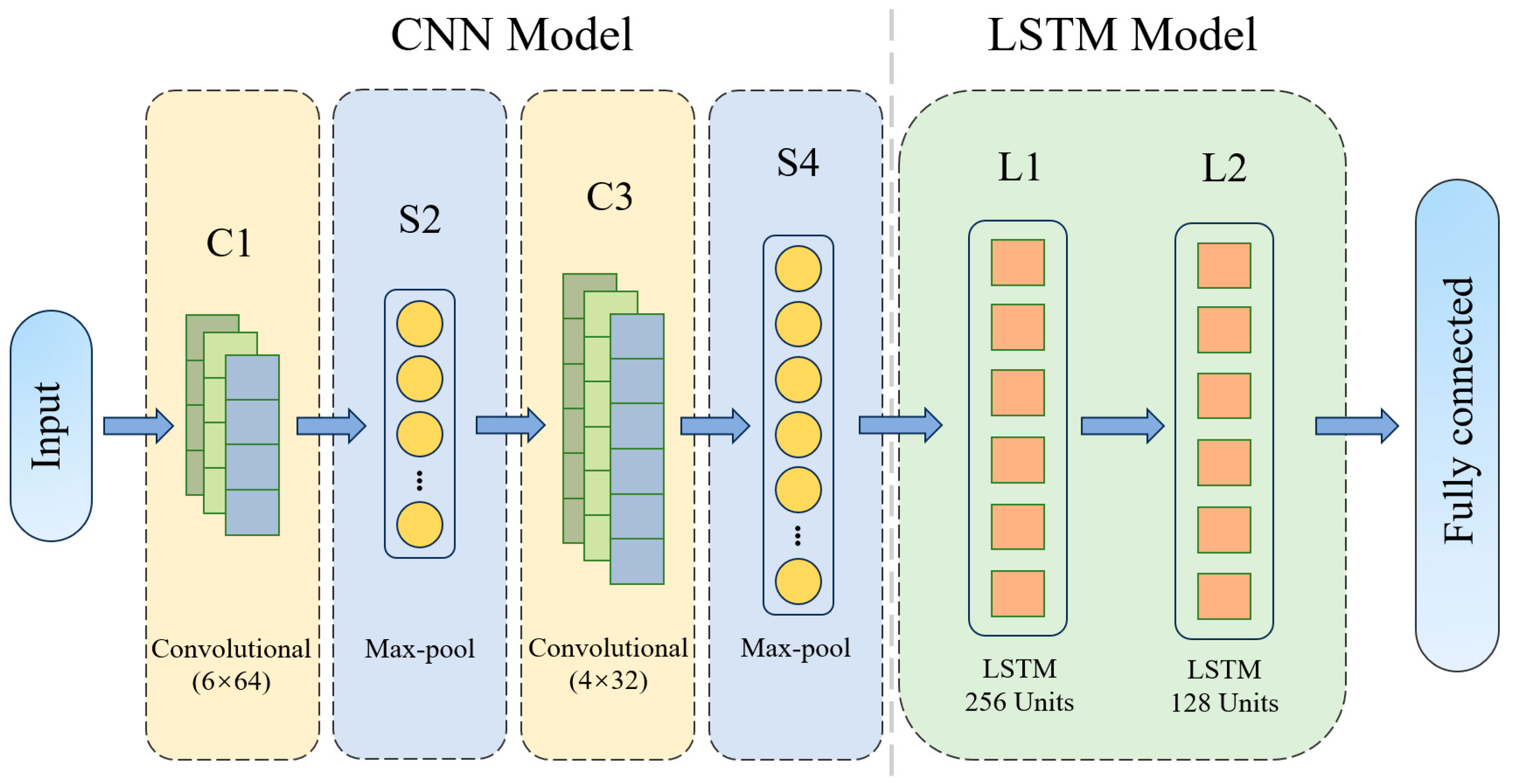
3.1. Construction of a CNN–LSTM-Based Maize Seedling Quality-Grading Model
3.1.1. CNN Network Architecture
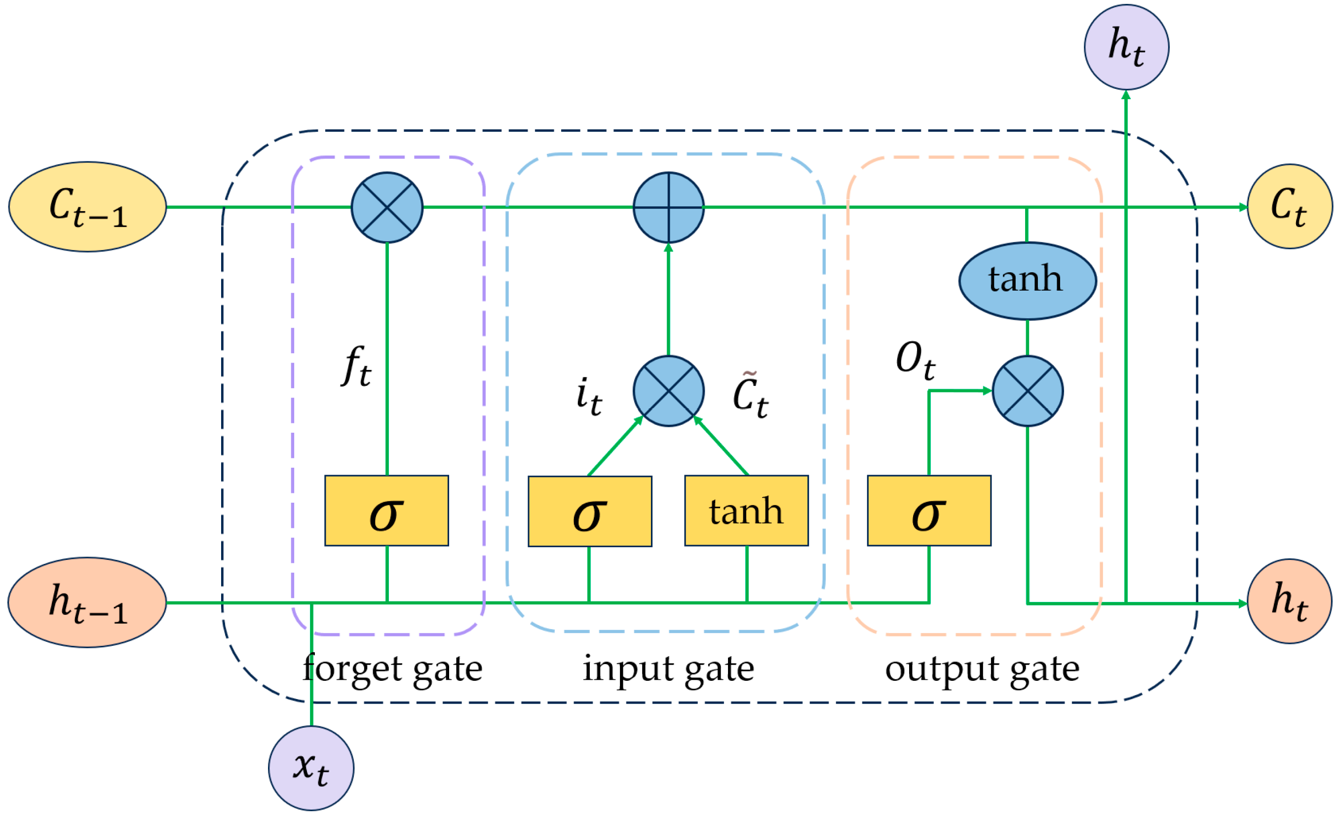
3.1.2. LSTM Network Structure
- Forget Gate. It is used to regulate the information in the memory unit from the preceding time step, which requires elimination. Using the forget gate, the LSTM unit can forget previous irrelevant information and retain only useful information. The forget gate assesses the and , when , and the information is discarded; however, when is used, the information is preserved. The formula for iswhere represents the weight of the forget gate, signifies the activation function, and defines the bias factor for the forget gate.
- Input Gate. It retains new information within the long-term state, comprising three components: initially, the layer generates a new vector of candidate values; subsequently, the input gate layer regulates the elements requiring updates; and ultimately, the new information is incorporated into the long-term state, represented by the following formula:where denotes the candidate value generated by the layer, and are the weight matrices of the memory cells, and is the bias coefficient of the memory cells. and denote the weight matrices of the input gates, denotes the activation function, denotes the bias coefficients of the input gates, is the input, and is the output.
- Output Gate. It regulates information retrieved from the memory cell for the current output. Initially, the output information is ascertained by the sigmoid layer, followed by processing of the long-term state by the layer, which is multiplied by the information filtered through the output gate to yield the final result. The output vector of the output gate is computed aswhere denotes the sigmoid activation function; and are the weight matrices of the output gates; and is the bias coefficient of the output gates.
3.1.3. Optimiser
| Algorithm 1: optimiser |
| Input: , , , |
| Initialise: , , |
| While do |
| was the gradient of the time step |
| was the first moment of the step |
| was the second moment of the step |
| , were the exponential decay rate coefficients |
| End while |
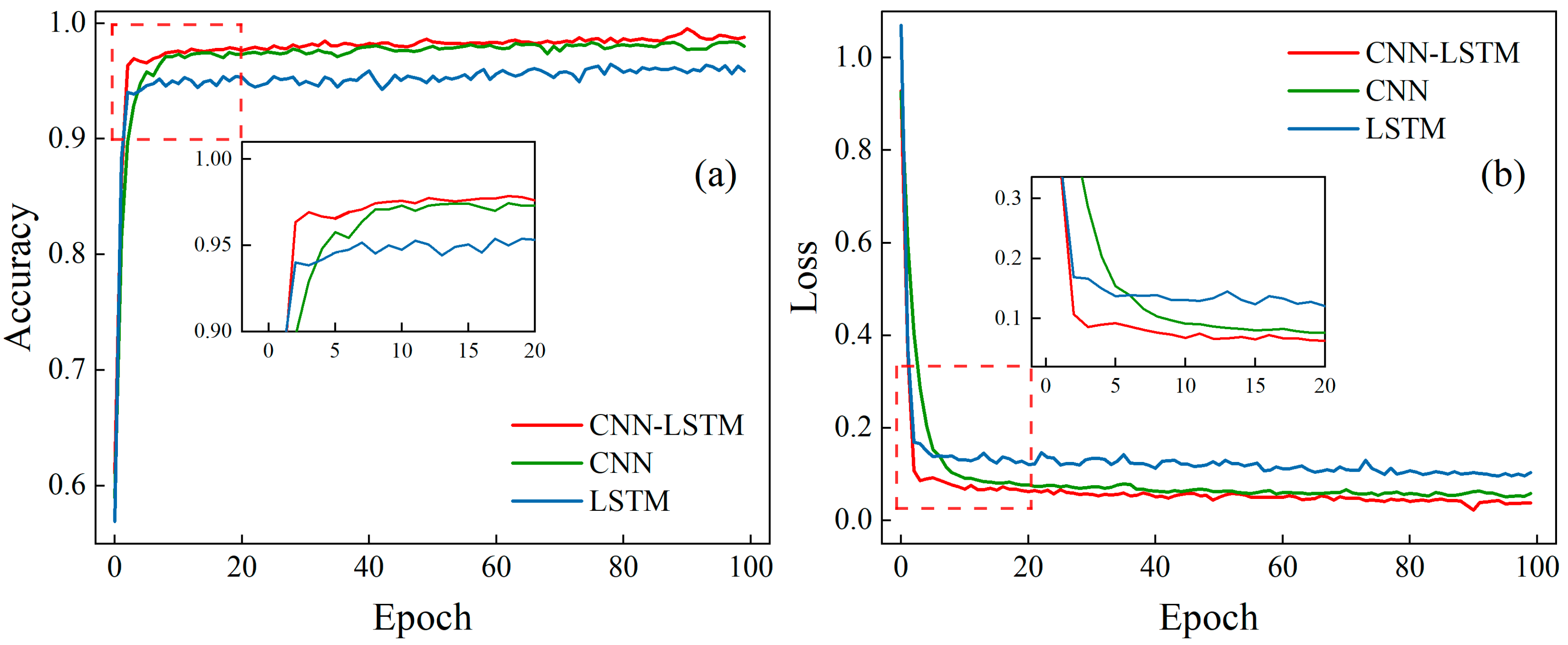
3.2. Model Training
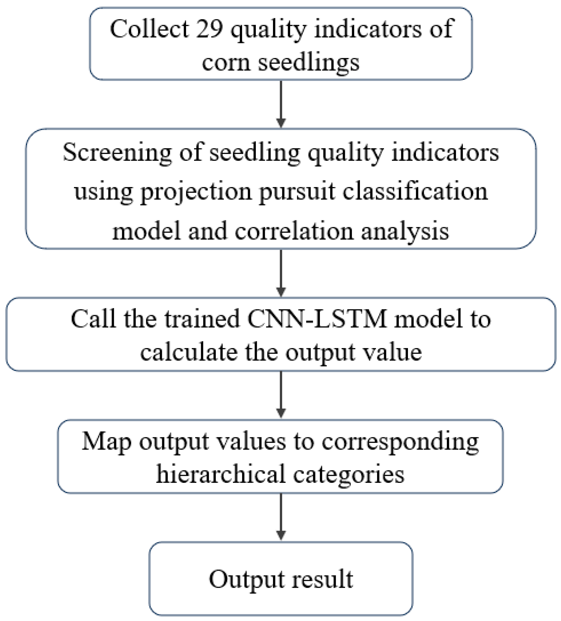
3.3. Model Simulation Testing
4. Discussion
4.1. Model Performance Evaluation
4.2. Limitations
4.3. Future Research Directions
5. Conclusions
Author Contributions
Funding
Data Availability Statement
Acknowledgments
Conflicts of Interest
References
- Han, X.; Dong, L.; Cao, Y.; Lyu, Y.J.; Shao, X.W.; Wang, Y.J.; Wang, L.C. Adaptation to climate change effects by cultivar and sowing date selection for maize in the Northeast China Plain. Agronomy 2022, 12, 984. [Google Scholar] [CrossRef]
- Zhao, J.; Yang, X.G.; Liu, Z.J.; Lv, S.; Wang, J.; Dai, S.W. Variations in the potential climatic suitability distribution patterns and grain yields for spring maize in Northeast China under climate change. Clim. Chang. 2016, 137, 29–42. [Google Scholar] [CrossRef]
- Jiang, R.; He, W.T.; He, L.; Yang, J.Y.; Qian, B.; Zhou, W.; He, P. Modelling adaptation strategies to reduce adverse impacts of climate change on maize cropping system in Northeast China. Sci. Rep. 2021, 11, 810. [Google Scholar] [CrossRef] [PubMed]
- Lin, Y.M.; Feng, Z.M.; Wu, W.X.; Yang, Y.Z.; Zhou, Y.; Xu, C.C. Potential impacts of climate change and adaptation on maize in Northeast China. Agron. J. 2017, 109, 1476–1490. [Google Scholar] [CrossRef]
- Zhang, J.Y.; Li, Y.C.; Zhang, Z.W.; Di, H.; Zhang, L.; Wang, X.R.; Wang, Z.H.; Zhou, Y. Combining ability and genetic diversity under low-temperature conditions at germination stage of maize (Zea mays L.). Euphytica 2021, 217, 125. [Google Scholar] [CrossRef]
- Zhao, Y.M.; Na, M.L.; Guo, Y.; Liu, X.P.; Tong, Z.J.; Zhang, J.Q.; Zhao, C.L. Dynamic vulnerability assessment of maize under low temperature and drought concurrent stress in Songliao Plain. Agric. Water Manag. 2023, 286, 108400. [Google Scholar] [CrossRef]
- Fan, D.J.; Song, D.P.; Jiang, R.; He, P.; Shi, Y.Y.; Pan, Z.L.; Zou, G.Y.; He, W.T. Modelling adaptation measures to improve maize production and reduce soil N2O emissions under climate change in Northeast China. Atmos. Environ. 2024, 319, 120241. [Google Scholar] [CrossRef]
- Li, X.F.; Guo, Q.G.; Gong, L.J.; Jiang, L.X.; Zhai, M.; Wang, L.L.; Wang, P.; Zhao, H.Y. Impact assessment of maize cold damage and drought cross-stress in Northeast China based on WOFOST model. Int. J. Plant Prod. 2024, 18, 1–12. [Google Scholar] [CrossRef]
- Qi, X.; Wan, C.; Zhang, X.; Sun, W.F.; Liu, R.; Wang, Z.; Wang, Z.N.; Ling, F.L. Effects of histone methylation modification on low temperature seed germination and growth of maize. Sci. Rep. 2023, 13, 5196. [Google Scholar] [CrossRef] [PubMed]
- Nguyen, H.T.; Leipner, J.; Stamp, P.; Guerra-Peraza, O. Low temperature stress in maize (Zea mays L.) induces genes involved in photosynthesis and signal transduction as studied by suppression subtractive hybridization. Plant Physiol. Biochem. 2009, 47, 116–122. [Google Scholar] [CrossRef] [PubMed]
- Li, S.X.; Yang, W.Y.; Guo, J.H.; Li, X.N.; Lin, J.X.; Zhu, X.C. Changes in photosynthesis and respiratory metabolism of maize seedlings growing under low temperature stress may be regulated by arbuscular mycorrhizal fungi. Plant Physiol. Biochem. 2020, 154, 1–10. [Google Scholar] [CrossRef] [PubMed]
- Lu, H.; Xia, Z.; Fu, Y.; Wang, Q.; Xue, J.; Chu, J. Response of soil temperature, moisture, and spring maize (Zea mays L.) root/shoot growth to different mulching materials in semi-arid areas of Northwest China. Agronomy 2020, 10, 453. [Google Scholar] [CrossRef]
- Xia, Z.; Zhang, G.; Zhang, S.; Wang, Q.; Fu, Y.; Lu, H. Efficacy of root zone temperature increase in root and shoot development and hormone changes in different maize genotypes. Agriculture 2021, 11, 477. [Google Scholar] [CrossRef]
- Li, L.J.; Gu, W.R.; Li, C.F.; Meng, Y.; Mu, J.Y.; Guo, Y.L.; Li, J.; Wei, S. Effect of DCPTA on antioxidant system and osmotic adjustment substance in leaves of maize seedlings under low temperature stress. Plant Physiol. J. 2016, 52, 1829–1841. Available online: https://link.cnki.net/doi/10.13592/j.cnki.ppj.2016.0138 (accessed on 20 December 2016).
- Gao, C.H.; Hu, J.; Zheng, Y.Y.; Zhang, S. Antioxidant enzyme activities and proline content in maize seedling and their relationships to cold endurance. Chin. J. Appl. Ecol. 2006, 6, 1045–1050. Available online: https://www.cjae.net/CN/abstract/abstract1204.shtml (accessed on 30 June 2006).
- Hu, S.L.; Sanchez, D.L.; Wang, C.L.; Lipka, A.E.; Yin, Y.H.; Gardner, C.A.C.; Lübberstedt, T. Brassinosteroid and gibberellin control of seedling traits in maize (Zea mays L.). Plant Sci. 2017, 263, 132–141. [Google Scholar] [CrossRef] [PubMed]
- Wang, Y.; Zhang, X.Y.; Chen, J.; Chen, A.J.; Wang, L.Y.; Guo, X.Y.; Niu, Y.L.; Liu, S.R.; Mi, G.H.; Gao, Q. Reducing basal nitrogen rate to improve maize seedling growth, water and nitrogen use efficiencies under drought stress by optimizing root morphology and distribution. Agric. Water Manag. 2019, 212, 328–337. [Google Scholar] [CrossRef]
- Yang, M.; Yang, J.; Su, L.; Sun, K.; Li, D.X.; Liu, Y.Z.; Wang, H.; Chen, Z.Q.; Guo, T. Metabolic profile analysis and identification of key metabolites during rice seed germination under low-temperature stress. Plant Sci. 2019, 289, 110282. [Google Scholar] [CrossRef] [PubMed]
- Kumar, R.; Chug, A.; Singh, A.P. Plant foliage disease diagnosis using light-weight efficient sequential CNN model. Opt. Mem. Neural Netw. 2023, 32, 331–345. [Google Scholar] [CrossRef]
- Sahu, K.; Minz, S. Adaptive segmentation with intelligent ResNet and LSTM–DNN for plant leaf multi-disease classification model. Sens. Imaging 2023, 24, 22. [Google Scholar] [CrossRef]
- Asiri, Y. Unmanned aerial vehicles assisted rice seedling detection using shark smell optimization with deep learning model. Phys. Commun. 2023, 59, 102079. [Google Scholar] [CrossRef]
- Qi, H.N.; Huang, Z.H.; Jin, B.C.; Tang, Q.Z.; Jia, L.Q.; Zhao, G.W.; Cao, D.D.; Sun, Z.Y.; Zhang, C. SAM-GAN: An improved DCGAN for rice seed viability determination using near-infrared hyperspectral imaging. Comput. Electron. Agric. 2024, 216, 108473. [Google Scholar] [CrossRef]
- Hao, X.; Jia, J.D.; Gao, W.L.; Guo, X.C.; Zhang, W.X.; Zheng, L.H.; Wang, M.J. MFC-CNN: An automatic grading scheme for light stress levels of lettuce (Lactuca sativa L.) leaves. Comput. Electron. Agric. 2020, 179, 105847. [Google Scholar] [CrossRef]
- Maginga, T.J.; Masabo, E.; Bakunzibake, P.; Kim, K.S.; Nsenga, J. Using wavelet transform and hybrid CNN–LSTM models on VOC & ultrasound IoT sensor data for non–visual maize disease detection. Heliyon 2024, 10, e26647. [Google Scholar] [CrossRef]
- Zhuang, S.; Wang, P.; Jiang, B.R.; Li, M.S. Learned features of leaf phenotype to monitor maize water status in the fields. Comput. Electron. Agric. 2020, 172, 105347. [Google Scholar] [CrossRef]
- Liu, X.; Cao, K.; Li, M. Assessing the impact of meteorological and agricultural drought on maize yields to optimize irrigation in Heilongjiang Province, China. J. Clean Prod. 2024, 434, 139897. [Google Scholar] [CrossRef]
- Guga, S.; Bole, Y.; Riao, D.; Bilige, S.; Wei, S.; Li, K.; Zhang, J.; Tong, Z.; Liu, X. The challenge of chilling injury amid shifting maize planting boundaries: A case study of Northeast China. Agr. Syst. 2025, 222, 104166. [Google Scholar] [CrossRef]
- Itroutwar, P.D.; Kasivelu, G.; Raguraman, V.; Malaichamy, K.; Sevathapandian, S.K. Effects of biogenic zinc oxide nanoparticles on seed germination and seedling vigor of maize (Zea mays). Biocatal. Agric. Biotechnol. 2020, 29, 101778. [Google Scholar] [CrossRef]
- Li, Y.; Zhang, Y.; Yang, K.; Lu, Y.; Wu, G.; Liu, H.; Liu, Y. Effects of freeze injury with different phases and various durations between sowing and seedling periods on growth and resistant physiological of maize seedlings. J. Maize Sci. 2022, 30, 73–82. [Google Scholar] [CrossRef]
- Evans, T.; Griscom, H. Comparing the effects of four propagation methods on hybrid chestnut seedling quality. Trees Forest. People 2021, 6, 100157. [Google Scholar] [CrossRef]
- Zhang, M.Y.; Qi, Q.; Zhang, D.J.; Tong, S.Z.; Wang, X.H.; An, Y.; Lu, X.G. Effect of priming on Carex schmidtii seed germination and seedling growth: Implications for tussock wetland restoration. Ecol. Eng. 2021, 171, 106389. [Google Scholar] [CrossRef]
- Liu, Y.; Guo, L.; Huang, Z.; López-Vicente, M.; Wu, G.L. Root morphological characteristics and soil water infiltration capacity in semi-arid artificial grassland soils. Agric. Water Manag. 2020, 235, 106153. [Google Scholar] [CrossRef]
- Chiango, H.; Figueiredo, A.; Sousa, L.; Sinclair, T.; da Silva, J.M. Assessing drought tolerance of traditional maize genotypes of Mozambique using chlorophyll fluorescence parameters. S. Afr. J. Bot. 2021, 138, 311–317. [Google Scholar] [CrossRef]
- Zhang, L.Y.; Han, W.T.; Niu, Y.X.; Chávez, J.L.; Shao, G.M.; Zhang, H.H. Evaluating the sensitivity of water stressed maize chlorophyll and structure based on UAV derived vegetation indices. Comput. Electron. Agric. 2021, 185, 106174. [Google Scholar] [CrossRef]
- Ma, J.F.; Chen, Y.P.; Wang, K.B.; Huang, Y.Z.; Wang, H.J. Re-utilization of Chinese medicinal herbal residues improved soil fertility and maintained maize yield under chemical fertilizer reduction. Chemosphere 2021, 283, 131262. [Google Scholar] [CrossRef] [PubMed]
- Zhang, Y.F.; Lu, Y.X.; Guan, H.O.; Yang, J.; Zhang, C.Y.; Yu, S.; Li, Y.C.; Guo, W.; Yu, L.H. A phenotypic extraction and Deep Learning-Based method for grading the seedling quality of maize in a cold region. Agronomy 2024, 14, 674. [Google Scholar] [CrossRef]
- Bai, Y.; Shi, W.H.; Xing, X.J.; Wang, Y.; Jin, Y.R.; Zhang, L.; Song, Y.F.; Dong, L.H.; Liu, H.B. Study on tobacco vigorous seedling indexes model. Sci. Agric. Sin. 2014, 6, 1086–1098. [Google Scholar] [CrossRef]
- Wu, X.L.; Zhang, Y.H. Coupling analysis of ecological environment evaluation and urbanization using projection pursuit model in Xi’an, China. Ecol. Indic. 2023, 156, 111078. [Google Scholar] [CrossRef]
- Fu, Q.; Xie, Y.G.; Wei, Z.M. Application of projection pursuit evaluation model based on real-coded accelerating genetic algorithm in evaluating wetland soil quality variations in the Sanjiang plain, China. Pedosphere 2003, 13, 249–256. [Google Scholar]
- Zhang, N.; Tan, Q.Y.; Song, W.C.; Li, Q.Y. Optimization of above-ground environmental factors in greenhouses using a multi-objective adaptive annealing genetic algorithm. Heliyon 2024, 10, e33036. [Google Scholar] [CrossRef] [PubMed]
- Pei, W.; Hao, L.; Fu, Q.; Ren, Y.T.; Li, T.X. Study on spring drought in cold and arid regions based on the ANOVA projection pursuit model. Ecol. Indic. 2024, 160, 111772. [Google Scholar] [CrossRef]
- Yan, J.H.; Ren, K.; Wang, T. Improving multidimensional normal cloud model to evaluate groundwater quality with grey wolf optimization algorithm and projection pursuit method. J. Environ. Manag. 2024, 354, 120279. [Google Scholar] [CrossRef]
- Semenoglou, A.A.; Spiliotis, E.; Assimakopoulos, V. Image-based time series forecasting: A deep convolutional neural network approach. Neural. Netw. 2023, 157, 39–53. [Google Scholar] [CrossRef] [PubMed]
- Chen, F.; Shen, Y.; Li, G.L.; Ai, M.; Wang, L.; Ma, H.Z.; He, W.D. Classification of wheat grain varieties using terahertz spectroscopy and convolutional neural network. J. Food Compos. Anal. 2024, 129, 106060. [Google Scholar] [CrossRef]
- Karki, S.; Basak, J.K.; Tamrakar, N.; Deb, N.C.; Paudel, B.; Kook, J.H.; Kang, M.Y.; Kang, D.Y.; Kim, H.T. Strawberry disease detection using transfer learning of deep convolutional neural networks. Sci. Hortic. 2024, 332, 113241. [Google Scholar] [CrossRef]
- Bai, Z.H. Residential electricity prediction based on GA-LSTM modeling. Energy Rep. 2024, 11, 6223–6232. [Google Scholar] [CrossRef]
- Ishida, K.; Ercan, A.; Nagasato, T.; Kiyama, M.; Amagasaki, M. Use of one-dimensional CNN for input data size reduction in LSTM for improved computational efficiency and accuracy in hourly rainfall-runoff modeling. J. Environ. Manag. 2024, 359, 120931. [Google Scholar] [CrossRef] [PubMed]
- Zhang, Z.Y.; Tian, J.W.; Huang, W.Z.; Yin, L.R.; Zheng, W.F.; Liu, S. A haze prediction method based on one-dimensional convolutional neural network. Atmosphere 2021, 12, 1327. [Google Scholar] [CrossRef]
- Moitra, D.; Mandal, R.K. Classification of non-small cell lung cancer using one-dimensional convolutional neural network. Expert Syst. Appl. 2020, 159, 113564. [Google Scholar] [CrossRef]
- Lu, X.Q.; Tian, J.; Liao, Q.; Xu, Z.W.; Gan, L. CNN-LSTM based incremental attention mechanism enabled phase-space reconstruction for chaotic time series prediction. J. Electron. Sci. Technol. 2024, 22, 100256. [Google Scholar] [CrossRef]
- Yu, M.; Ma, X.D.; Guan, H.O.; Zhang, T. A diagnosis model of soybean leaf diseases based on improved residual neural network. Chemom. Intell. Lab. Syst. 2023, 237, 104824. [Google Scholar] [CrossRef]
- Yang, J.; Ma, X.D.; Guan, H.O.; Yang, C.; Zhang, Y.F.; Li, G.B.; Li, Z.S.; Lu, Y.X. A quality detection method of corn based on spectral technology and deep learning model. Spectrochim. Acta A Mol. Biomol. Spectrosc. 2024, 305, 123472. [Google Scholar] [CrossRef] [PubMed]
- Wang, Q.; Xia, Z.Q.; Zhang, S.B.; Fu, Y.F.; Zhang, G.X.; Lu, H.D. Elevated temperature during seedling stage in different maize varieties: Effect on seedling growth and leaf physiological characteristics. Russ. J. Plant Physiol. 2022, 69, 138. [Google Scholar] [CrossRef]
- Li, G.Y.; Ma, Z.W.; Zhang, N.; Li, M.; Li, W.; Mo, Z.W. Foliar application of silica nanoparticles positively influences the early growth stage and antioxidant defense of maize under low light stress. J. Soil Sci. Plant Nutr. 2024, 24, 2276–2294. [Google Scholar] [CrossRef]
- Haque, M.A.; Marwaha, S.; Deb, C.K.; Nigam, S.; Arora, A.; Hooda, K.S.; Soujanya, P.L.; Aggarwal, S.K.; Lall, B.; Kumar, M.; et al. Deep learning-based approach for identification of diseases of maize crop. Sci. Rep. 2022, 12, 6334. [Google Scholar] [CrossRef] [PubMed]


| Quality Indicators of Seedlings | Number | Quality Indicators of Seedlings | Number | Quality Indicators of Seedlings | Number |
|---|---|---|---|---|---|
| Plant height | x1 | 3rd leaf length | x10 | F0 | x19 |
| Stem diameter | x2 | 3rd leaf width | x11 | Fm | x20 |
| Coleoptile length | x3 | Total leaf area | x12 | Fv/Fm | x21 |
| 1st leaf sheath length | x4 | Primary radicle length | x13 | Shoot fresh weight | x22 |
| 2nd leaf sheath length | x5 | Primary radicle diameter | x14 | Root fresh weight | x23 |
| 1st leaf length | x6 | Secondary radicle number | x15 | Residual seed fresh weight | x24 |
| 1st leaf width | x7 | Nodal root number | x16 | Shoot dry weight | x25 |
| 2nd leaf length | x8 | Root volume | x17 | Root dry weight | x26 |
| 2nd leaf width | x9 | SPAD value | x18 | Residual seed dry weight | x27 |
| Single Indicator | Projection Value | Single Indicator | Projection Value |
|---|---|---|---|
| Plant height (x1) | 0.85 ** | Secondary radicle number (x15) | 0.30 * |
| Stem diameter (x2) | 0.84 ** | Nodal root number (x16) | −0.39 * |
| Coleoptile length (x3) | 0.63 ** | Root volume (x17) | 0.72 ** |
| 1st leaf sheath length (x4) | 0.65 ** | SPAD value (x18) | 0.01 |
| 2nd leaf sheath length (x5) | 0.63 ** | F0 (x19) | −0.11 |
| 1st leaf length (x6) | 0.54 ** | Fm (x20) | −0.13 |
| 1st leaf width (x7) | 0.64 ** | Fv/Fm (x21) | −0.06 |
| 2nd leaf length (x8) | 0.68 ** | Shoot fresh weight (x22) | 0.84 ** |
| 2nd leaf width (x9) | 0.63 ** | Root fresh weight (x23) | 0.76 ** |
| 3rd leaf length (x10) | 0.56 ** | Residual seed fresh weight (x24) | −0.46 * |
| 3rd leaf width (x11) | 0.86 ** | Shoot dry weight (x25) | 0.65 ** |
| Total leaf area (x12) | 0.88 ** | Root dry weight (x26) | 0.65 ** |
| Primary radicle length (x13) | 0.23 | Residual seed dry weight (x27) | −0.47 * |
| Primary radicle diameter (x14) | −0.24 |
| Grade of Seedling Quality | Training Sets | Test Sets | Encoding Label |
|---|---|---|---|
| I | 918 | 305 | [1,0,0,0] |
| II | 864 | 288 | [0,1,0,0] |
| III | 702 | 234 | [0,0,1,0] |
| IV | 234 | 78 | [0,0,0,1] |
| Total | 2718 | 905 | -- |
| Model | Training Set | Test Set | ||||||
|---|---|---|---|---|---|---|---|---|
| Accuracy | Percentage Increase | Loss | Percentage Reduction | Accuracy | Percentage Increase | Loss | Percentage Reduction | |
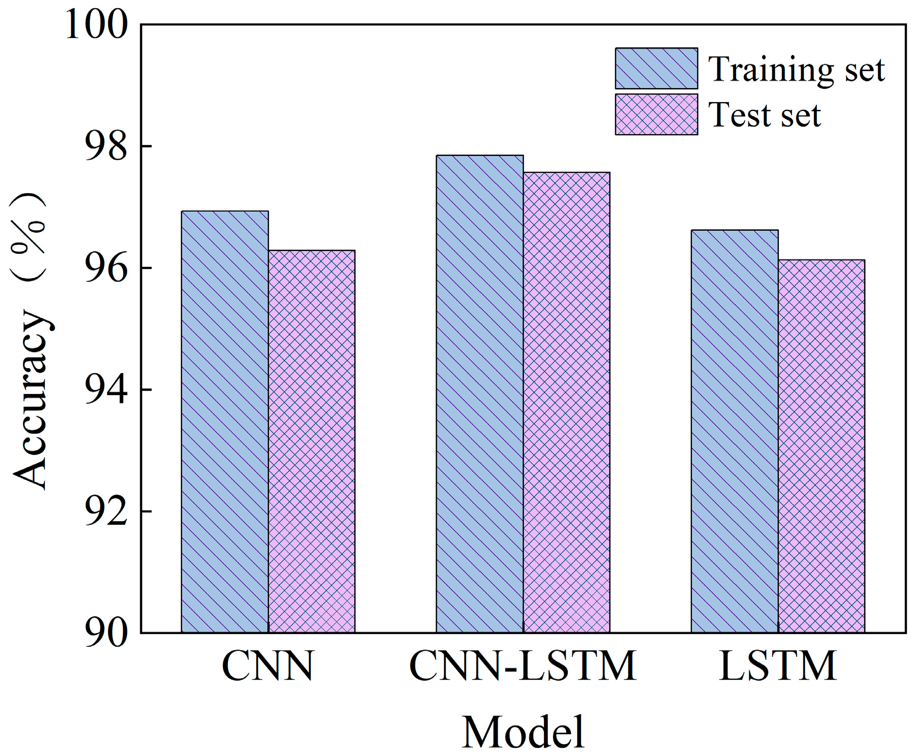
| CNN | 96.93% | 0.95% | 0.0909 | 34.67% | 96.29% | 1.33% | 0.0908 | 5.70% |
| LSTM | 96.62% | 1.27% | 0.1106 | 63.85% | 96.13% | 1.50% | 0.1312 | 52.74% |
| CNN–LSTM | 97.85% | — | 0.0675 | — | 97.57% | — | 0.0859 | — |
| Evaluation Seedling Grade | Training Set | Test Set | ||||
|---|---|---|---|---|---|---|
| Precision | Recall | F1 Score | Precision | Recall | F1 Score | |
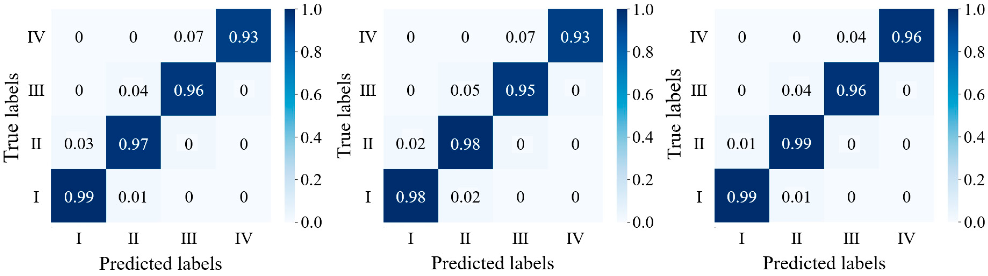
| Optimal seedling | 99.2% | 99.2% | 99.2% | 98.3% | 99.1% | 98.7% |
| Suboptimal seedling | 98.8% | 94.4% | 96.5% | 98.8% | 94.4% | 96.5% |
| Medium seedling | 95.8% | 98.9% | 97.3% | 95.8% | 98.9% | 97.3% |
| Weak seedling | 96.3% | 100.0% | 98.1% | 96.3% | 96.3% | 96.3% |
Disclaimer/Publisher’s Note: The statements, opinions and data contained in all publications are solely those of the individual author(s) and contributor(s) and not of MDPI and/or the editor(s). MDPI and/or the editor(s) disclaim responsibility for any injury to people or property resulting from any ideas, methods, instructions or products referred to in the content. |
© 2025 by the authors. Licensee MDPI, Basel, Switzerland. This article is an open access article distributed under the terms and conditions of the Creative Commons Attribution (CC BY) license (https://creativecommons.org/licenses/by/4.0/).
Share and Cite
Yu, S.; Lu, Y.; Zhang, Y.; Liu, X.; Zhang, Y.; Li, M.; Du, H.; Su, S.; Liu, J.; Yu, S.; et al. Development of an Efficient Grading Model for Maize Seedlings Based on Indicator Extraction in High-Latitude Cold Regions of Northeast China. Agronomy 2025, 15, 254. https://doi.org/10.3390/agronomy15020254
Yu S, Lu Y, Zhang Y, Liu X, Zhang Y, Li M, Du H, Su S, Liu J, Yu S, et al. Development of an Efficient Grading Model for Maize Seedlings Based on Indicator Extraction in High-Latitude Cold Regions of Northeast China. Agronomy. 2025; 15(2):254. https://doi.org/10.3390/agronomy15020254
Chicago/Turabian StyleYu, Song, Yuxin Lu, Yutao Zhang, Xinran Liu, Yifei Zhang, Mukai Li, Haotian Du, Shan Su, Jiawang Liu, Shiqiang Yu, and et al. 2025. "Development of an Efficient Grading Model for Maize Seedlings Based on Indicator Extraction in High-Latitude Cold Regions of Northeast China" Agronomy 15, no. 2: 254. https://doi.org/10.3390/agronomy15020254
APA StyleYu, S., Lu, Y., Zhang, Y., Liu, X., Zhang, Y., Li, M., Du, H., Su, S., Liu, J., Yu, S., Yang, J., Lv, Y., Guan, H., & Zhang, C. (2025). Development of an Efficient Grading Model for Maize Seedlings Based on Indicator Extraction in High-Latitude Cold Regions of Northeast China. Agronomy, 15(2), 254. https://doi.org/10.3390/agronomy15020254