Abstract
The application of autonomous navigation in intelligent agriculture is becoming more and more extensive. Traditional navigation schemes in greenhouses, orchards, and other agricultural environments often have problems such as the inability to deal with an uneven illumination distribution, complex layout, highly repetitive and similar structures, and difficulty in receiving GNSS (Global Navigation Satellite System) signals. In order to solve this problem, this paper proposes a new tightly coupled LiDAR (Light Detection and Ranging) inertial odometry SLAM (LIO-SAM) framework named April-LIO-SAM. The framework innovatively uses Apriltag, a two-dimensional bar code widely used for precise positioning, pose estimation, and scene recognition of objects as a global positioning beacon to replace GNSS to provide absolute pose observation. The system uses three-dimensional LiDAR (VLP-16) and IMU (inertial measurement unit) to collect environmental data and uses Apriltag as absolute coordinates instead of GNSS to solve the problem of unreliable GNSS signal reception in greenhouses, orchards, and other agricultural environments. The SLAM trajectories and navigation performance were validated in a carefully built greenhouse and orchard environment. The experimental results show that the navigation map developed by the April-LIO-SAM yields a root mean square error of 0.057 m. The average positioning errors are 0.041 m, 0.049 m, 0.056 m, and 0.070 m, respectively, when the density of Apriltag is 3 m, 5 m, and 7 m. The navigation experimental results indicate that, at speeds of 0.4, 0.3, and 0.2 m/s, the average lateral deviation is less than 0.053 m, with a standard deviation below 0.034 m. The average heading deviation is less than 2.3°, with a standard deviation below 1.6°. The positioning stability experiments under interference conditions such as illumination and occlusion were carried out. It was verified that the system maintained a good stability under complex external conditions, and the positioning error fluctuation was within 3.0 mm. The results confirm that the robot positioning and navigation accuracy of mobile robots satisfy the continuity in the facility.
1. Introduction
Autonomous navigation technology has been widely used in modern agriculture, especially in complex environments such as greenhouses and orchards, and its importance has become increasingly prominent [1]. The special environmental conditions in the greenhouse, such as narrow crop row spacing, large illumination changes, weak Global Navigation Satellite System signals, and the random distribution of obstacles, put forward extremely high requirements for the accuracy and reliability of the autonomous navigation system. Traditional navigation schemes, such as fixed orbit navigation and tracking navigation, can achieve autonomous navigation to a certain extent, but they have problems such as high costs and poor flexibility, which make it difficult to meet the complex needs of the greenhouse environment [2]. Therefore, multi-source data fusion navigation technology based on Simultaneous Localization and Mapping (SLAM) technology has gradually become the development direction of autonomous navigation technology for agriculture due to its advantages of high environmental adaptability, real-time navigation and obstacle avoidance, and no need to lay a fixed track [3]. At present, the autonomous navigation technology applied to facility agriculture can be mainly divided into three categories: fixed track, guided tracking, and multi-source data fusion based on SLAM technology. Fixed track is the most structured approach, where the robot’s path is physically or virtually constrained. It includes systems that follow pre-defined physical tracks, buried wires, or magnetic tapes. While offering a high reliability in repetitive tasks, it lacks flexibility and is unsuitable for dynamic or unstructured environments. The guided tracking navigation scheme includes beacon and landmark navigation. It is more concerned about ‘whether it can successfully reach the target point’, and which way to go is secondary. But the fixed trajectory tracking is concerned with ‘whether to strictly follow a given line’; such systems include systems in which the robot infers its path by tracking an external reference or beacon without physical constraints. A classic example is beacon-based navigation, which relies on a network of pre-installed artificial markers, such as Radio Frequency Identification (RFID), Bluetooth Low Energy (BLE), and Wi-Fi. Key examples include BLE for proximity and fingerprinting-based localization [4], Wi-Fi for an efficient indoor positioning system [5], and RFID for indoor dynamic positioning [6]. Another example is landmark navigation, such as GPS for in-motion coarse alignment using position loci [7]. Multi-source data fusion navigation methods based on SLAM are mainly classified as visual SLAM and laser SLAM navigation. Fusion processing usually makes use of LiDAR, camera, encoder, gyroscope, and other sensor information to achieve autonomous navigation. These navigation methods do not need to arrange the installation of a track, guide line, or base station, which saves the cost of initial installation and increases the scope of application and activity space of the navigation system [8]. However, the application of multi-source data fusion navigation based on SLAM technology in facility agriculture is still scarce, and the application of the 3D laser SLAM algorithm with higher robustness and accuracy is scarcer [9,10]. LiDAR-based SLAM has gained attention for its stability and robustness against lighting variations. Researchers have developed 2D/3D LiDAR-SLAM solutions to reduce computational load and improve mapping accuracy. However, in densely planted greenhouses, the presence of unstructured crops and irregular gaps can complicate the extraction of clear geometric features (e.g., walls, rows), leading to ambiguous map boundaries [11]. Furthermore, during seasons with sparse canopy coverage, the reduced structural features can adversely affect the accuracy of map matching and long-term positioning. While sensor fusion techniques, such as integrating ultrasonic technology [12], Ultra-Wideband (UWB) [13,14], IMU, and machine vision [15,16], have been employed to mitigate the accumulation of errors over time, challenges like positioning accuracy fluctuations and mapping distortions due to environmental symmetries persist. These limitations indicate that the existing SLAM solutions still struggle to achieve the high-precision, stable, and long-distance navigation required for reliable robotic operations in complex greenhouse environments. Although the application of SLAM technology in agricultural facilities has been explored, the existing technology, especially the navigation scheme based on two-dimensional laser SLAM and visual SLAM, still has difficulty in solving the problems of mapping distortion caused by similar characteristics between crop rows in facilities and the accumulation of positioning accuracy errors caused by rough roads [17]. Alhmiedat et al. [18] developed a SLAM navigation system based on an adaptive Monte Carlo localization (AMCL) algorithm for sensor-constrained Pepper robots. By fusing LiDAR and odometer data, an average positioning accuracy of 0.51 m is achieved in the indoor environment. However, such filter-based SLAM methods are prone to cumulative errors due to sensor noise and feature matching failure in long-strip and sparse greenhouse environments, resulting in map distortions and long-term positioning drift. In order to overcome the influence of illumination on visual navigation, Jiang et al. [19] innovatively fused the thermal imaging camera with a 2D laser and used the YOLACT deep learning algorithm to achieve navigation under low-light and no-light conditions. The average position error in the orchard is 0.20 m. This study shows the great potential of cross-modal perception. However, this kind of pure perception scheme still has problems such as difficulties in feature extraction and the failure of closed-loop detection when dealing with highly similar and unstructured crop ridges, and cumulative error is still a chronic disease that is difficult to completely solve. In view of the inherent limitations of natural feature SLAM, researchers have begun to re-examine and innovate the role of the ‘external beacon’, upgrading it from the original navigation core to a high-precision benchmark to assist the SLAM system in correcting cumulative errors. Traditional beacon navigation (such as low-cost GNSS-RTK used by Baltazar et al. [20]) is limited by signal occlusion and insufficient accuracy, and it is difficult to apply directly in greenhouses. However, the new generation of artificial visual beacons, such as Apriltag, provides an ideal tool for solving the cumulative error problem of SLAM because of their high recognition, computational efficiency, and ability to provide centimeter-level absolute pose information. Apriltag is a vision-based positioning technology that achieves high-precision 6-degree-of-freedom positioning by detecting specially designed 2D tags [21]. It has the characteristics of high robustness, high precision, and fast detection, and is suitable for robot navigation, drone positioning, augmented reality, and industrial automation. However, it also has shortcomings such as field angle limitation, distance limitation, and a dependence on visual sensors [22]. Compared with UWB and other devices, Apriltag has the advantage of low cost, and its hardware is mainly composed of ordinary cameras and self-printable tags. Its installation is easy to realize, and the label can be affixed to a variety of surfaces. The camera can be installed on robots, drones, or other equipment. The system has the advantage of flexible integration. It can be integrated with a variety of sensors, such as IMU and odometers, to form a more complete positioning system [23]. Zhang et al. [24] proposed a new method combining visual labeling and a factor graph by using Apriltag technology. Through multi-factor constraints and graph optimization, the accuracy and robustness of localization are significantly improved. This method can maintain centimeter-level positioning accuracy at different speeds and meet the operation requirements of agricultural robots. However, only the visual inertial factor graph optimization system based on Apriltag is used. The role of IMU here is to provide smooth constraints on inter-frame motion and help overcome image blur and short-term occlusion. However, the absolute positioning ability of the system comes entirely from the observations of Apriltag. It will be completely lost when the mark is not visible. The accurate use of specific markers in visual navigation by Chen et al. [25] also indirectly proves the reliability of highly recognizable artificial features in complex environments. Tan et al. [26] proposed a SLAM navigation system that integrates LiDAR and ultrasonic tags, which significantly improves the positioning robustness and accuracy in a repetitive structure environment. The system remains stable under high-speed motion. At a speed of 0.6 m/s, the maximum lateral error of navigation is 0.045 m, and the average lateral error is 0.022 m. This paper proposes adding Apriltag as a correction factor to LIO-SAM to build a more powerful, more general, and closer to industrial application. It makes up for the vulnerability of visual markers with the strong robustness of LiDAR and makes up for the systematic drift of LiDAR in a specific environment with the absolute accuracy of visual markers. The system can continue to work without being completely lost, even if all the markers are temporarily invisible.
In summary, there are many problems in achieving autonomous navigation in agricultural facilities such as greenhouses and orchards. The current two-dimensional laser SLAM and visual SLAM navigation schemes often cause mapping deviations due to similar characteristics between crop rows and accumulate positioning errors due to uneven roads. This study focuses on the autonomous navigation scenarios of greenhouses and orchards and proposes a positioning and navigation scheme based on the fusion of tightly coupled LiDAR inertial odometry via smoothing, mapping, and Apriltag, aiming to solve the problem of wheel odometer error accumulation and the similarity of environmental characteristics and finally realize the high-precision positioning and navigation of an agricultural scene autonomous walking system.
This paper presents a systematic approach to enhance LiDAR inertial SLAM in GNSS-denied environments by integrating visual fiducial markers. The main innovations and contributions are as follows:
- A General Framework for Visual-Enhanced LiDAR Inertial Odometry: This work presents a principled methodology for embedding sparse but high-fidelity visual fiducial markers into a tightly coupled LiDAR inertial odometry framework. The core contribution is to propose a method of integrating the Apriltag factor instead of the original GNSS factor into the factor graph, which provides global constraints and cumulative error correction for the robot in the GNSS-denied environment. By designing a tightly coupled Apriltag factor within the LIO-SAM backbone, we achieve more than just the substitution of GNSS. The system is specifically engineered to handle the intermittent nature of visual observations, effectively leveraging sporadic tag detections to correct long-term drift without relying on continuous GNSS signals. This approach effectively bridges the gap between dense, relative LiDAR measurements and sparse, absolute visual detections, establishing a generalizable paradigm for enhancing state estimation in GNSS-denied environments beyond the specific case of Apriltags.
- A Systematic Deployment Framework for Visual Fiducial Makers: A key contribution of this work is to transform the deployment of tags from a temporary process to a systematic, principle-driven practice. Through rigorous experiments, we established a quantitative relationship between tag spacing and positioning accuracy. We determined that the spacing of 3 m is an optimal balance point, which can achieve centimeter-level accuracy (0.06 m RMSE) while ensuring actual deployment efficiency. In addition, this study further proposes a systematic deployment strategy: the vertical bracket is used to deploy Apriltag vertically, and its spatial density can be flexibly adjusted according to different positioning accuracy requirements. This strategy fundamentally reduces the complexity and cost of large-scale deployment, making scalable and reliable deployment possible in a broad agricultural environment.
- Comprehensive Experimental Validation: We provide a thorough quantitative evaluation of the system’s performance. Analogy experiments simulating real-world experiments were conducted to rigorously validate not only the superior localization accuracy (achieving centimeter-level precision with dense tag deployment) but also the robustness and reliability of Apriltag detection under varying lighting conditions and viewing angles. This empirical validation offers strong evidence for the reliability and practicality of our proposed approach.
The rest of this paper is structured as follows: Section 2 describes the construction of the mobile detection platform used in this paper, introduces the proposed tightly coupled LiDAR inertial visual SLAM framework in detail, including the overall system architecture, data fusion method, Apriltag pose factor design and integration, map construction, and global positioning implementation details, describes the experimental design and setting. Section 3 and Section 4 analyzes the experimental results and discusses the factors affecting positioning accuracy in the study. Section 5 summarizes the research in this paper and gives directions for future improvement.
2. Materials and Methods
2.1. Mobile Robot Composition
The efficient operation of the greenhouse or orchard autonomous navigation system depends on a mobile robot platform that can adapt to complex environments and has high-precision positioning and navigation capabilities. The platform not only needs to drive between the narrow crop rows in the greenhouse, but also needs to stably complete the function of positioning and navigation in an environment with weak GNSS signals and strong illumination changes. Therefore, this paper integrates and develops a set of complex agricultural environment autonomous mapping robot systems. The system consists of a controller, a mobile chassis, and an environment-aware system. The hardware structure of the autonomous mapping robot is shown in Figure 1.
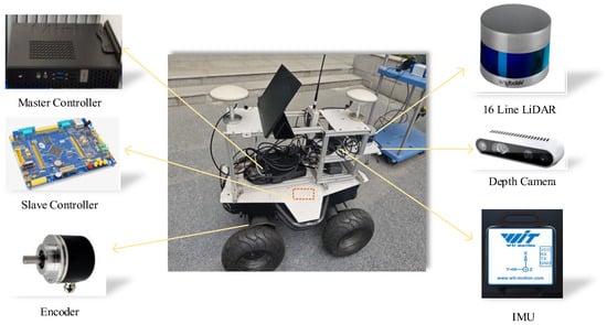
Figure 1.
Mobile robot hardware structure diagram.
2.2. Construction of the Moving Platform
2.2.1. Environmental Awareness Module
The mobile platform is equipped with a three-dimensional LiDAR (Velodyne, VLP-16, Velodyne LiDAR Inc., San Jose, CA, USA) and a nine-axis high-frequency inertial measurement unit (Witte, wit-hwt901, Shenzhen, China) to obtain the distance information of objects in the environment and posture of the platform. The Velodyne VLP-16 is a 16-beam mechanical rotating LiDAR system. It employs 16 vertically aligned laser emitters and receivers to perform 360° rotational scanning, utilizing the Time-of-Flight (ToF) principle to accurately perceive the environment and generate three-dimensional point cloud data. The maximum scanning distance is 100 m. Recognized for its revolutionary balance between performance and favorable cost-effectiveness, this sensor enabled real-time mid-to-long-range 3D environmental perception. It has been extensively deployed in autonomous vehicle development, robotic navigation, and 3D mapping applications, making seminal contributions to the advancement of related technological fields. The depth camera is a D435 (Intel Corp, Santa Clara, CA, USA). The minimum detection range is 0.105 m and the maximum one is about 10.0 m. It can provide high-resolution depth images with a high accuracy and is suitable for applications that require high-depth information, such as object recognition and three-dimensional reconstruction. The inertial measurement unit employed in this system is the WIT901 model, which features a triaxial accelerometer with a measurable range of ±16 g and a triaxial gyroscope capable of detecting angular velocities up to ±2000°/s. The attitude output ranges are ±180° for the roll (X) and yaw (Z) axes and ±90° for the pitch (Y) axis. The measured static accuracy of the attitude angles is 0.2° for the X and Y axes and 1° for the Z axis. The magnetometer range is ±49 Gauss, the nonlinearity is ±0.2% FS, and the noise density is 3 mGauss. The sensor outputs triaxial acceleration, triaxial angular velocity, and triaxial magnetic field data at a frequency of 200 Hz.
2.2.2. Chassis Module
The mobile platform uses a two-wheel differential drive system, with an encoder for each driving motor of the wheel to obtain the motion information of the platform in real time. Through the proportional–integral–differential control algorithm, the real-time speed is used as feedback information to improve the speed control accuracy. CAN communication is selected as the communication method. The detailed parameters of the chassis and the driving system can be found in Table A1 and Table A2 in Appendix A.
2.3. Mobile Robot Detection Platform Software Design
The software system architecture of the mobile robot is shown in Figure 2, which is divided into two major parts: the upper computer and the lower one. The upper computer software runs on the ROS(Melodic), and the software program mainly includes the sensor data processing function package and the navigation function package. The sensor data processing function package is used to realize the data acquisition and fusion calculation of the sensor, and the calculated corrected pose and IMU are output to the navigation function package. The sensor data processing function package consists of two parts: camera data processing and LiDAR data processing. Camera data processing includes the camera node, Apriltag node, and pose calculation node. LiDAR data processing includes 3D LiDAR nodes and RF2O nodes. The navigation function package is used to realize positioning and navigation, including the mapping node, localization node, and path-planning node. The real-time data transmission between the above ROS nodes is realized by the topic message communication mechanism based on the ‘publish/subscribe’ model [27]. The lower computer software runs on the embedded controller, which is responsible for receiving the linear velocity and angular velocity information issued by the upper computer, and outputs the control signal through the calculation program to drive and control the robot to walk and turn. The data communication between the upper computer and the lower computer is carried out through CAN/2.0B standard protocol, and the message format is in MOTOROLA format. The technical roadmap is shown in Figure 3.

Figure 2.
Mobile robot software system architecture.
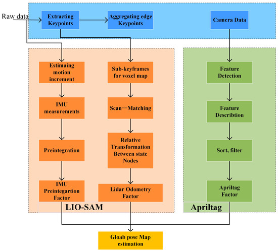
Figure 3.
Technical roadmap of navigation systems based on the integration of LiDAR and Apriltag.
2.4. Realization Principle of Autonomous Mapping and Navigation Function of Mobile Robot
2.4.1. Multi-Sensor Calibration and Time Synchronization
In order to achieve high-precision positioning, it is necessary to complete the necessary preparatory work to meet the accuracy requirements. The first step is to calibrate the internal parameters of the IMU, aiming to solve its inherent measurement errors. In this study, the imu_utils [28] toolbox developed by professor Shen Shaojie of Hong Kong University of Science and Technology was used for calibration, and four key calibration parameters were obtained. Multi-sensor joint calibration is the premise of realizing the spatial synchronization of different sensors and lays the foundation for data fusion. Specifically, the LiDAR_imu_calib [29] tool developed by professor Liu Yong of Zhejiang University is used to complete the external parameter calibration of LiDAR and IMU, and the spatial transformation relationship between the two coordinate systems is determined, which is characterized by a translation vector and a rotation matrix. The time synchronization between LiDAR and IMU data is realized by the built-in time synchronization mechanism of ROS. The mechanism automatically aligns the timestamp in the process of topic message publishing and subscribing, which ensures the accurate synchronization of data between sensors and provides an accurate and reliable basis for subsequent data fusion and processing.
The autonomous walking system needs to avoid collision with crop ridges when going straight and turning. However, due to the poor signal in the greenhouse, the traditional GNSS positioning may not work normally. The uneven ground may cause the wheels of the mobile platform to slip sideways, and the real-time positioning deviation of the traditional SLAM algorithm may be large. At the same time, the similarity of inter-row environmental features may be high, and single-line LiDAR cannot provide rich point cloud data [13]. Therefore, maps constructed by traditional 2D SLAM algorithms such as gmapping and cartographer will be severely distorted [30]. In order to solve this problem, the LIO-SAM [31] algorithm is selected as the SLAM scheme. Compared with FAST-LIO [32], although it is highly efficient and robust, it is essentially a filter that usually does not contain or only has a simple loopback detection module. In the absence of structured features or in the presence of a large number of similar scenarios (such as long corridors and dense forests), cumulative drift is difficult to be effectively eliminated. Although VINS-Fusion [33] is an excellent visual inertial SLAM, its LiDAR version is essentially a loosely coupled fusion scheme. The performance will be affected when visual failures (such as sudden illumination changes and texture loss) or point clouds are sparse. The mapping process includes point cloud preprocessing, feature detection and matching, loop closure detection, and dimension reduction processing. The schematic diagram is shown in Figure 4.

Figure 4.
April-LIO-SAM schematic diagram.
2.4.2. Point Cloud Preprocessing
The original point cloud data often contain outliers and noise caused by dust, haze, sensor errors, and other factors, which will seriously interfere with the subsequent geometric feature extraction. This paper uses a two-step method for data cleaning, and the specific process is shown in Figure 5.

Figure 5.
Point cloud processing sequence diagram.
Firstly, the obvious invalid points are quickly eliminated by setting the distance threshold. The point cloud within the effective measurement range is retained, and its mathematical expression is as follows:
where and represent the minimum and maximum effective distance thresholds, which are set to 0.5 m and 8.5 m, respectively, in this study. represents the filtered point cloud. represents the raw cloud.
In order to further remove the scattered noise points, an outlier removal filter based on statistics (SOR) is used. The algorithm is based on the distribution characteristics of the point cloud in the local neighborhood [34]. A point cloud set containing N points is given, where each point is a three-dimensional vector. For each point , we find its K nearest neighbors and calculate the Euclidean distance from the point to the K nearest neighbors. Then, the average distance is calculated:
Supposing that the average distance of normal points obeys Gaussian distribution, the global mean and standard deviation of the average distance of all points are calculated.
Set a distance threshold interval based on global statistics; if the average distance of a point exceeds this interval, it is determined to be an outlier and removed.
The amount of clean point cloud data is still huge. In order to reduce the computational burden and make the point cloud distribution more uniform, the voxel grid filter is used for downsampling. Calculate the centroid of these neighborhood points. The centroid represents the center position of the spatial distribution of these K points [35]. For a point , the calculation formula is as follows:
where is the calculated mean point (centroid), K is the number of selected nearest neighbor points, and are the coordinates of the j-th nearest neighbor point.
The voxel filter is used to downsample the point cloud data to reduce the amount of data and improve the computational efficiency. The point cloud set after filtering and downsampling is expressed as follows (M is filtered point number): , .
The ground point cloud removal mainly uses the random sample consensus (RANSAC) method. Randomly select a small number of samples from the point cloud set as the interior point candidate set (c is the number of point clouds as candidate interior points).
In order to solve the problem of inaccurate ground segmentation in complex terrains (such as slopes and walls) using the traditional RANSAC method, this study introduces the gravity direction provided by IMU as an a priori constraint. First, the direction of the gravity vector in the LiDAR coordinate system is extracted from the IMU data [36]. Assuming that the gravity vector is , the corresponding ground reference plane normal vector can be expressed as follows:
In the RANSAC plane fitting process, the angle constraint is applied to the candidate plane normal vector generated by each random sampling:
where θ is the maximum allowable angle deviation (set to 20°), and the plane is accepted as a valid ground candidate plane only when the angle between the normal vector of the candidate plane and the reference gravity direction is less than this threshold.
The function fit_model (C) of ground plane model fitting is used to fit the ground plane model of the candidate set C of interior points. According to the fitted ground plane model and the threshold distance df, the vertical distance from all data points to the model is calculated. The data points less than the threshold df are regarded as interior points, and the number of interior points is expressed as follows:
The optimal interior point set Iinlier is selected repeatedly according to the maximum number of interior points, and Iinlier is removed as a ground point. Finally, during the movement of the mobile platform, due to the presence of attitude changes and unstable factors, the data collected by the LiDAR may be affected by motion distortion, which has a negative impact on the accuracy of mapping and positioning. In order to solve this problem, the LIO-SAM algorithm uses the inertial measurement unit to measure the attitude and acceleration information of the platform. By jointly optimizing the pose information and the LiDAR data, the laser points are aligned in time to correct the data distortion of the LiDAR.
2.4.3. Feature Detection and Matching
The LIO-SAM algorithm uses a curvature-based feature detection method to extract geometric features from LiDAR data. The curvature value is used to measure the sharpness or change rate of point cloud data. According to the curvature in one scanning cycle, the point cloud is classified. The points with a larger curvature are divided into edge features, and the points with a smaller curvature are divided into plane features. Using the method referenced in [37], the calculation of the i-th curvature Ci is shown in the following formula:
In the formula, k represents the complete scanning period of the k-th LiDAR; L is the current coordinate frame of LiDAR; and i is the index of the target point for which the curvature is being calculated. S is the set of consecutive points of point i returned by the laser scanner in the same scan. represents the three-dimensional coordinates of the target point i in the LiDAR coordinate system L and in the scanning period k. represents the three-dimensional coordinates of the adjacent point i in the LiDAR coordinate system L in the scanning period k. Finally, RANSAC feature matching estimation is used to estimate the model parameters of feature points, and error matching is filtered to realize map building and robot pose tracking in the SLAM task [38].
Apriltag is a visual benchmark marking system based on two-dimensional code topology. Its positioning process is divided into three steps:
- (1)
- Label detection and decoding
Edge segmentation: The local adaptive binarization of image I is performed as follows:
where and are the mean and standard deviation of pixels in the sliding window, and = 0.3 is the empirical coefficient.
- (2)
- Homography matrix solution
Let the label corner homogeneous coordinate and the image coordinate satisfy the following:
- (3)
- Pose estimation
The rotation matrix and the translation vector of the camera to the label are obtained by decomposing the homography matrix H:
where is the column vector of H, and . is the standard basis vector .
2.4.4. Factor Graph Construction
The core of this system is based on the factor graph optimization framework of LIO-SAM. The key innovation is to replace the original GNSS factor with a novel Apriltag one to provide absolute pose constraints so as to effectively correct the inherent cumulative drift in the laser inertial odometer without relying on external satellite signals.
- (1)
- Factor graph model construction
The goal of back-end optimization is to estimate the optimal sequence of robot states (pose and speed) , usually containing the robot’s pose, , and speed. This is achieved by constructing a factor graph , where the node represents the unknown state variable to be estimated and the factor represents the probability constraint between these state variables measured by the sensor [39].
The optimal state estimation is obtained by maximizing the joint probability of all factors, which is equivalent to solving a nonlinear least squares problem:
where is the residual of the factor for a given measurement , and is the square of the Mahalanobis distance under the covariance matrix , representing the measurement uncertainty. In the original LIO-SAM, the factor set mainly includes the IMU pre-integration factor, a constraint between the continuous state and derived from the IMU data; the laser odometry factor, a ‘search match’ constraint from asynchronous states; the closed-loop factor, which identifies the constraints of the access location; and the GNSS factor (to be replaced), which provides an absolute position constraint .
- (2)
- From GNSS factor to Apriltag factor
Replacing the GNSS factor with the Apriltag one is the core contribution of this work, which transforms a sparse position-only constraint into a dense full pose constraint.
The original scheme GNSS factor provides the noise measurement of the robot’s global position . The residual function of the GNSS factor attached to the state is simply the difference between the measured position and the predicted position of the state estimation:
is the translation component of pose . This residual is a 3-dimensional vector. A significant limitation is that it only constrains the position of the robot and does not provide any orientation information.
The coordinate relationship in the positioning system is shown in Figure 6. When an Apriltag is detected, it provides an accurate 6-DOF transformation from the tag coordinate system to the camera coordinate system to measure T_. Given the external parameter transformation between the calibrated camera and the LiDAR and the global pose pre-measured by the tag in the world coordinate system W, we can calculate an absolute pose measurement of the robot at time k:
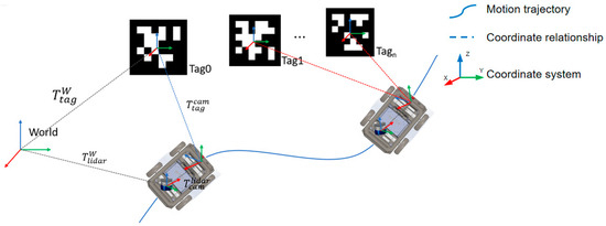
Figure 6.
The coordinate relationship in the positioning system.
The derived measured value is used as the observed value of our new factor. The residuals of the Apriltag factor are computed by the Lie algebra operator () formulated [40] in the tangent space of :
The residual is a 6-dimensional vector (3-dimensional rotation, 3-dimensional translation), which quantifies the difference between the estimated pose and the absolute measurement pose [41]. Compared with the GNSS factor, this provides a much stronger state constraint, effectively correcting both the position drift and the rotation (yaw) drift, and is the main error source of the odometer system.
The covariance matrix of the factor is very important. It reflects the uncertainty of visual inspection, which is usually a function of the distance from the tag to the camera, its direction relative to the optical axis, and the image resolution. This allows the optimizer to automatically weigh the confidence of each Apriltag observation relative to other constraints in the graph.
- (3)
- Integration factor graph
The overall objective function of the optimization system is changed into the following:
With as the residual of IMU, as the residual of Apriltag, as the residual of LiDAR, and as the residual of the closed loop.
As long as the tag is detected, the Apriltag factor is added to the graph to provide intermittent but high-precision absolute correction. The incremental solver iSAM2 effectively integrates these new constraints and updates the entire trajectory estimation to ensure global consistency in an environment equipped with visual markers.
2.5. Performance Experiments
2.5.1. Experimental Equipment and Materials
The performance evaluation indexes of the autonomous walking system mainly include the accuracy of SLAM, system positioning accuracy, and system navigation accuracy. The mapping accuracy refers to the matching degree between the size of the grid map and the actual scene size; the system positioning accuracy is the deviation between the position information obtained by the specified bit algorithm and the actual position. System navigation accuracy refers to the deviation between the preset path generated by the mobile platform and the actual motion path. The experiment is divided into two parts. The test scene is set in the school playground and the forest part to simulate the greenhouse environment and the hilly orchard part, respectively.
The simulated greenhouse environment (called Scene1 in the rest of this paper) is 25 m long and 8 m wide, including three ridges and four cultivation shelves. The inter-row feature similarity is high, and the experimental scene is shown in Figure 7a. The orchard environment (called Scene2 in the rest of this paper) is selected in the forest area in Jiangsu University. The ground is uneven, and the ground slope is different. The experimental scene is shown in Figure 7b.
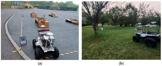
Figure 7.
Field experiment scene diagram; (a) Experimental scene greenhouse. (b) Experimental scene orchard diagram.
It should be noted that the RTK system is only used to provide a reliable true position value, and it does not participate in any positioning and navigation procedure in the proposed method. The RTK base station system is shown in Figure 8.
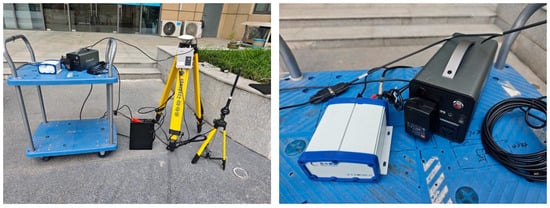
Figure 8.
Schematic diagram of base station system.
The production of Apriltag tags: The Apriltag tag is generated using the OpenMV IDE platform (OpenMV LLC, Cambridge, MA, USA) through a software-generated method. Selecting the TAG36H11 family in the Apriltag generator of the software’s machine vision can easily generate the required series of independently numbered Apriltag tags.
In designing the layout of the Apriltag label, this study considers various forms of achieving efficient, stable, and flexible label deployment in a complex agricultural environment. The first scheme is to post Apriltag tags on the ground. The advantage of this scheme is that the camera can quickly identify the tags and respond. However, the ground tags are easily affected by pollutants such as dust and soil, resulting in a decrease in positioning accuracy. In addition, the ease of posting on the ground is not enough. If it needs to be reused in other locations, it must be re-posted. Scheme 2 is to post Apriltag tags at specific locations (such as walls, columns, or cultivation shelves). Through plastic packaging treatment, it can resist fouling to a certain extent and protect the clarity and durability of the label. However, this kind of layout still has the problem of poor flexibility and has difficulty adapting to the changing agricultural operation scenarios. In view of the limitations of the above two schemes, this study finally tends to Scheme 3, that is, using vertical brackets to arrange Apriltag tags. Practice has proved that the vertical bracket can effectively avoid the fouling problem and greatly improve the flexibility of the label arrangement. In different agricultural facility environments, vertical supports can be quickly deployed without complex installation processes. In addition, by placing the label in a relatively open and less occluded position, the detection success rate of the label is significantly improved to ensure that the mobile platform can obtain the positioning information stably and accurately. This innovative layout scheme not only enhances the environmental adaptability of the system but also reduces the maintenance cost, which provides strong support for the promotion and application of agricultural navigation technology.
The layout of Apriltag tags should be flexibly planned according to specific application scenarios and environmental characteristics. In the greenhouse environment, it is recommended to use an equal spacing arrangement along the crop rows because it is highly matched with the structural features of the greenhouse rules, the deployment process is simplified. The spacing can be adjusted according to the actual density of the crop, and it is usually recommended to be controlled within 10 m. This arrangement helps to reduce the visual blind area and ensure that an effective overlapping area can be formed between adjacent tags during the scanning process, thereby maintaining the continuity and stability of the positioning. In the layouts in the relevant literature, which include the placement of Apriltag tags at the corners of the site and the placement of eight tags around the boundary, these experiences provide an important reference for this experiment. In order to explore the optimal arrangement distance of Apriltag tags in Scene1, the distance between Apriltags, ds, is set with different values, and each arrangement scheme was systematically tested. In Scene2, in addition to arranging labels between rows, additional labels should be added between trees to prevent signal loss in certain areas due to tree occlusion, so as to ensure the accuracy of positioning. This layout strategy considering environmental characteristics aims to improve the detection efficiency and positioning reliability of tags in complex agricultural environments.
In order to ensure the high precision and reliability of the experiment, the GNSS RTK (real-time kinematic measurement) system is used as the positioning reference. The RTK system can provide centimeter-level positioning accuracy in real time through the cooperative work of satellite signals and ground base stations, which greatly improves the accuracy of location data [42]. During the experiment, the RTK system will be used as a key positioning tool to provide accurate reference data for the driving path of the mobile robot. This not only helps to accurately measure the straight offset of the robot but also provides high-quality data support for subsequent navigation and control algorithm optimization. By using the RTK system, the straight-line driving performance of the robot can be evaluated more accurately, thus laying a solid foundation for the further improvement and development of the robot.
2.5.2. Comparison Test of Map Accuracy in Different Scenarios and Methods
In these experiments, the remote control terminal is used to control the autonomous mapping navigation robot, allowing it to travel in the experimental scene at a speed of 0.3 m/s, arrange Apriltag tags every 3.0 m, and detect and collect the information of 3D LiDAR, nine-axis IMU, and the monocular camera. The maps are constructed using the LIO-SAM, Gmapping, and April-LIO-SAM (the method proposed in this paper) algorithms, respectively. Seven positions are selected according to reference [30], and the absolute positions are obtained using RTK.
Regarding the establishment of a coordinate system, the corresponding definition is provided. Taking Scene1 as an example, an edge point in the experimental scene is recorded and its latitude and longitude are measured with RTK (119.50849415,32.20064772), using the method in Ref. [43]. Then, the converted UTM coordinates are recorded (x_rtk, y_rtk, z_rtk). At the same time, the initial attitude of the robot at this time (roll, pitch, yaw angle (φ, θ, ψ) in the UTM coordinate system) is recorded. This initial attitude is crucial, as it defines the orientation of the local odom coordinate system relative to the UTM coordinate system. The X axis is defined as pointing to the initial front of the robot. Then, the Y axis points to the initial left side of the robot (right hand rule). According to the initial attitude angle (φ, θ, ψ) and the initial position (x_rtk, y_rtk, z_rtk), a 4 × 4 homogeneous transformation matrix T (homogeneous transformation matrix) is constructed:
where c and s represent the cos and sin functions, respectively.
For the GNSS measurement value of any subsequent time point t, it is first converted from the latitude and longitude (LLA) to the UTM coordinate to obtain a point P_UTM = (x_rtk, y_rtk, z_rtk). In order to obtain the coordinate P_odom of the point in the odom coordinate system, it is necessary to invert the transformation matrix T and then apply the inverse transformation:
The obtained P_odom is the coordinate in the local Cartesian coordinate system with the starting point of the robot as the origin and the X-Y plane as the ground plane. The coordinates are converted with the entrance as the base point; seven static feature points (named as Pt1 to Pt7 in the rest of this paper), which are easy to recognize in the laser point cloud, are selected in the greenhouse. The best choices are as follows: corner root, fixed metal column foundation, permanent markers on the ground, etc. By attaching eye-catching markers (such as cross points) to each point, it is ensured that both the RTK centering rod and the laser point cloud are accurately aligned to the same position. Firstly, the RTK equipment (Beijing UniStrong Science & Technology Co., Ltd., Beijing, China) is used to measure and position the RTK centering rod accurately in the center of each marker point. After waiting for RTK to reach the fixed solution state, the three-dimensional coordinates of the point in the UTM coordinate system (x_rtk, y_rtk, z_rtk) are recorded. This is the ‘true position value’ of the point. Repeat this operation for all marker points to form a list of true value coordinates. Then, start the LIOSAM + Apriltag system designed in this paper; walk in the experimental scene and ensure that all the deployed landmarks are scanned and that the system also detects the deployed Apriltags and saves the final global point cloud map constructed by the system (usually in pcd format). Finally, use the point cloud processing software (CloudCompare, 2.14.alpha version) to enlarge the point cloud, find and select the corresponding position of the same marker point on the point cloud with the RTK measurement, and use the software’s ‘ranging’ tool to measure the center of the target surface. Record the coordinates of this point in the point cloud map (x_map, y_map, z_map) and repeat this operation for all check points. For each check point i, calculate its Euclidean distance error:
where , , represent the coordinates of the target point in the point cloud map, and , represent the three-dimensional coordinates of the target point in the UTM coordinate system measured by the RTK equipment.
After obtaining the Euclidean distance error, for each check point i, the Mean error and RMSE can be calculated:
where n represents the number of selected points, and represents the Euclidean distance error calculated above.
The layouts of Apriltag tags and selected static feature points are shown in Figure 9 for Scene1 and Scene2.
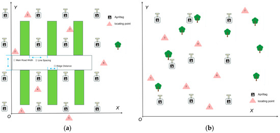
Figure 9.
Schematic diagram of map measurement points; (a) Schematic diagram of map Scene1. (b) Schematic diagram of map Scene2.
The constructed map effect is shown in Figure 10 and Figure 11; some markers can be seen (such as Apriltag, scaffold, bush), with blue arrows showing the one-to-one correspondence.
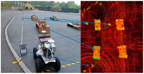
Figure 10.
The effect of April-LIO-SAM Scene1 mapping.
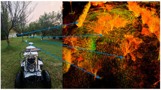
Figure 11.
The effect of April-LIO-SAM Scene2 mapping.
On the robot visualization (rviz) platform, the positions of Pt1–7 are obtained and calculated with the data of RTK measurement, and the absolute error, relative error, and root mean square error of the three mapping algorithms are obtained.
2.5.3. Testing the Relationship Between Tag Distance and Positioning Accuracy
In order to ensure the high precision and reliability of the experiments, different ds values are set as 3.0 m, 5.0 m, 7.0 m, and 10.0 m, respectively. By recording the positioning data of the robot at these positions and comparing with the actual positions, the offsets are calculated, and then the positioning accuracy of the combination of LIO-SAM and Apriltag is evaluated, which provides data support for the subsequent system optimization. The environmental factors are strictly controlled during the experiment, and the equipment is calibrated accurately to improve the credibility of the test results. The data measured in the two scenarios are recorded, and the trajectory data of RTK and the trajectory pairs output by LIO-SAM are shown in Figure 12. In order to study the effectiveness of adding Apriltag as a global constraint to the factor graph proposed in this paper, evo (Evolutionary Algorithm, https://github.com/MichaelGrupp/evo (accessed on 17 July 2025)), a Python3.13 package for the evaluation of odometry and SLAM, is used to evaluate positioning accuracy. The relative pose error (RPE) quantifies the accuracy of the estimated attitude relative to the real attitude in a fixed time interval and effectively evaluates the attitude result error. The RPE of frame i is the following:
where Ei represents the RPE of the i frame, Qi represents the true Apriltag pose value, Pi represents the estimated pose value, and ∆t represents a fixed interval time coefficient.
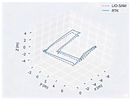
Figure 12.
Trajectory comparison diagram.
Suppose that the total number n and the interval are known; the n-∆t RPE values can be calculated. Then, we can use the root mean square error RMSE to count this error and obtain an overall value:
where represents the translation part of the RPE.
However, in the actual situation, we find that there are many choices for the selection of . In order to comprehensively measure the performance of the algorithm, we can calculate the average value of RMSE that traverses all :
2.5.4. Navigation Accuracy Experiments
As in the method of [25], the center line of the inter-row road in the test site is set as the target navigation path (Scene1), and the vehicle system travels along this path. A ridge is selected as the test environment, and the center line of the ridge is taken as the expected path. The vehicle system navigates autonomously along the preset path at the speeds of 0.20, 0.30, and 0.40 m/s; the lateral deviation and heading deviation are calculated by using the position coordinates and heading angle calculated by the robot in real time during autonomous navigation. Three experiments were carried out, respectively, and the maximum, average, and standard deviation of the lateral deviation and heading deviation were counted to evaluate the autonomous navigation performance of the mobile robot. The expansion radius of the obstacle is set to 0.5 m, the distance error limit between the center point of the robot and the target point on the x-y plane is set to 0.15 m, and the heading error limit is set to 0.2 rad.
The robot was commanded to navigate to the target position , and its actual position was measured as ; then, the lateral deviation is the following:
2.5.5. Apriltag Stability Experiments
In the case of outdoor interference, the system will give priority to the Apriltag detection algorithm and automatically switch to the occlusion target recognition algorithm when the target is under occlusion or other serious interference conditions. By analyzing the main interference factors of the outdoor environment, the most common and influential working environment conditions, such as different illuminations and occlusions, as well as different working distances, target positions (lateral displacement), and deflection angles, were selected for identification and positioning experiments [44]. The experiment is carried out on a high-precision translation stage. The Apriltag is installed on a precision-controlled dual-axis (X-Y) translation stage. The translation stage is driven by a stepper motor or a servo motor, and closed-loop feedback is performed through a grating ruler or a precision screw. The positioning accuracy can easily reach 0.01 mm or higher. The controller command translates the coordinates of the target position moved by the platform (for example, by 100.00 mm), and this value is the true value.
- (1)
- Occlusion experiments
The target may be partially occluded in the outdoor environment. In the experiments, we employed artificial occlusion to simulate potential occlusion scenarios, with the occlusion area set as 10%, 30%, and 50%, respectively. Success rate detection experiments were carried out a hundred times on the tags under different occlusion conditions at a vertical angle and a height of 0.5 m. Then, the working distance, the lateral distance, and the deflection angle of the target are changed to carry out the verification experiments to identify the positioning effect and positioning. The camera was fixed at 0.75 m (measured by laser range finder) above the vertical Apriltag, and the experiment was repeated ten times. The experimental diagram is shown in Figure 13.

Figure 13.
ApirlTag occlusion experiments. (a) Occlusion 10%; (b) Occlusion 30%; (c) Occlusion 50%.
- (2)
- Different illumination condition experiments
In the outdoor environment, the illumination conditions may be changing. In the experiments, the illumination intensity is increased from about 10 to 105 lx in turn. The light intensity was measured by a high-precision illumination sensor (0–157 k, LUX, RS485), and the camera was fixed at 0.75 m above the vertical Apriltag. The experiment was repeated ten times. At the same time, the working distance, the lateral distance of the target, and the deflection angle are changed to carry out the experiments. The experimental schematic diagram is shown in Figure 14.

Figure 14.
Different light intensity experiments. (a) Light intensity 10 lx; (b) Light intensity 102 lx; (c) Light intensity 103 lx; (d) Light intensity 104 lx; (e) Light intensity 105 lx.
- (3)
- Background interference and changing distance experiments
Various interference backgrounds, including a reflective background, clutter background, and multi-target interference, are applied in the outdoor environment, and the verification experiments are carried out by changing the working distance, the lateral distance, and the deflection angle of the target. We measured the positioning error under chaotic, two-target, and three-target interference. The positioning error within the distance of 1000–2000 mm is measured once every 200 mm. The experimental diagram is shown in Figure 15.
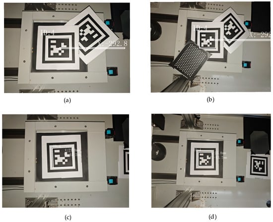
Figure 15.
Background interference experiments. (a) One interference; (b) Two interference; (c) 500 mm distance; (d) 1000 mm distance.
3. Results
3.1. The Results and Analysis of Map Construction with Different Methods
The accuracy of the three mapping algorithms is shown in Table 1.

Table 1.
Accuracy of three kinds of mapping in Scene1.
It can be seen that the accuracy of the Gmapping algorithm is the lowest, with a root mean square error (RMSE) of 0.630 m and an average error of 0.599 m. The results show that, as a pure laser SLAM algorithm based on a particle filter, Gmapping is susceptible to the cumulative error of LiDAR scanning matching in the absence of other sensor assistance, resulting in a limited mapping accuracy and difficulty in meeting the needs of high-precision applications. The performance of the LIO-SAM algorithm has been significantly improved. The RMSE is reduced to 0.372 m, and the average error is 0.316 m. This is due to its tightly coupled laser-IMU fusion framework. The IMU provides high-frequency pose change information, effectively constrains the cumulative error of scan matching, and maintains a higher stability in scenes with intense motion or missing features [45]. However, the error still reaches the decimeter level, indicating that the pure laser-IMU system still has the inherent drift problem. The April-LIO-SAM algorithm shows an overwhelming accuracy advantage. Its RMSE is only 0.057 m, and the average error is 0.049 m. The accuracy is one order of magnitude higher than that of LIO-SAM, reaching the centimeter level. This result fully proves the effectiveness of introducing a global, drift-free Apriltag visual reference point for closed-loop correction. This method successfully eliminates the cumulative error of the LIOM (laser inertial odometer) system and achieves globally consistent high-precision mapping. The experimental results show that the proposed method in this paper performs best in all the positions.
Due to the lack of features in the environment and high similarity in the two experimental sites, the uneven ground may lead to problems such as mobile site slippage, which will lead to the accumulation of distortion in the traditional SLAM algorithm relying on the LiDAR and odometer, resulting in the failure of mapping. However, the initial LIO-SAM algorithm lacks rich terrain features in the experimental site, which makes it difficult for the LiDAR to extract enough feature points for matching, affecting the positioning accuracy. At the same time, IMU errors will gradually accumulate in the absence of feature constraints, exacerbating positioning drift. If the system relies on GNSS correction, the GNSS signal difference will further reduce the global positioning accuracy and indirectly affect the LIO-SAM performance [46]. Since the Gmapping algorithm is a SLAM algorithm based on a particle filter, the robot position is mainly estimated by the characteristics of the laser scanning environment. The open environment lacks sufficient features (such as walls, obstacles, etc.), and the results of LiDAR scanning may be very sparse, even beyond the range of detecting, so it performs poorly in this environment.
3.2. Experimental Results and Analysis of Tag Distance and Positioning Accuracy
The positioning accuracy results obtained by the experiments are shown in Table 2.

Table 2.
Experimental results of positioning accuracy in different scenes.
From the experimental results, it can be seen that, when ds values are set as 3.0 m, 5.0 m, 7.0 m, and 10.0 m, respectively, the maximum deviations in the X direction and Y direction vary with the experimental scenes and the tag spacing. In Scene1, the maximum deviation in the X direction is 0.058 m, 0.098 m, 0.114 m, and 0.115 m, respectively, and in the Y direction is 0.073 m, 0.072 m, 0.096 m, and 0.094 m, respectively. In Scene2, the maximum deviations in the X and Y directions were 0.051, 0.057, 0.078, and 0.082 m and 0.046, 0.057, 0.068, and 0.102 m, respectively. The experimental results show that the deployment spacing of Apriltags has a decisive influence on the positioning accuracy and stability of the April-LIO-SAM system. Under the condition of dense deployment with a spacing of 3.0 m, the system achieves the best performance. The average positioning deviations in the X and Y directions are only 0.044 m and 0.052 m, respectively, and the standard deviations are the lowest (0.032 m and 0.027 m), which indicates that the system can provide high-precision and reproducible pose estimation. When the spacing increases to 7.0 m and 10.0 m, the positioning error shows a significant upward trend. The average deviations in the X and Y directions increase to 0.067 m and 0.084 m, respectively, and the standard deviation increases by more than 50%, reflecting the obvious degradation of positioning accuracy and consistency. Further analysis reveals that the system error has anisotropic characteristics. The accuracy in the Y direction (transverse) is more sensitive to the change in spacing, and the error increase is higher than that in the X direction (longitudinal). This suggests that the calibration accuracy of the external parameters of the sensor and the covariance setting in the pose graph optimization may be the key factors restricting the lateral performance. On the whole, because the terrain in the forest section is more complex and the feature points are rich, the positioning effect is better than that in Scene1, with fewer open feature points. It is more stable and closer to the lower limit than the original 5–12 cm, but the overall improvement of the positioning accuracy of the Apriltag tag is not as high as that of Scene1.
3.3. Navigation Accuracy Test Analysis
The navigation accuracy experiment results are shown in Table 3.

Table 3.
The result of navigation accuracy.
The navigation deviation in the X direction and the heading deviation at different speeds are shown in Figure 16.
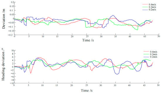
Figure 16.
Navigation deviation and heading deviation at different speeds.
From Table 3, it can be seen that, when the system is traveling at a speed of 0.2 m/s, the lateral deviation between the actual navigation path and the target path is less than 0.119 m, and the average angle error is 1.9°. When the system is traveling at a speed of 0.3 m/s, the lateral deviation between the actual navigation path and the target path is less than 0.116 m, and the average angle error is 1.8°. When the system is traveling at a speed of 0.4 m/s, the lateral deviation between the actual navigation path and the target path is less than 0.143 m, and the average angle error is 2.1°. Overall, at different speeds, the mean lateral deviation between the robot’s actual trajectory and the desired trajectory are less than 0.053 m, with standard deviations below 0.034 m. The mean heading deviation is consistently under 2.3°, and the standard deviation remains below 1.6°. Simultaneously, as the travel speed decreases, the standard deviations of both the lateral deviation and heading deviation gradually decrease, indicating a lower degree of dispersion between the robot’s navigation trajectory and the desired trajectory. In summary, at the three set speeds, the lateral deviation of the mobile robot’s autonomous navigation achieved a centimeter-level precision.
3.4. Results and Analysis of Apriltag Stability Experiments
The occlusion experiment results are shown in Figure 17 and Figure 18. From Figure 17, we can see that, when the occlusion is 10%, the recognition success rate is very high, reaching 96%. When the occlusion is 30%, the recognition success rate begins to decrease to 72%. When the occlusion is 50%, the recognition success rate decreases rapidly, reaching only 24%. The chart clearly shows that the recognition success rate of the Apriltag decreases sharply with the increase in occlusion area, especially after the occlusion is more than 30%; the success rate has dropped to a very low level, and the system becomes unstable. So, in practical application, the occlusion area should not exceed more than 50%, otherwise it may lead to the failure of recognition and positioning. From Figure 18a, the results show that the positioning errors of the system in the XY plane are less than 3.0 mm, the average error in the X direction is 2.3 mm, and the average error in the Y direction is 1.8 mm.
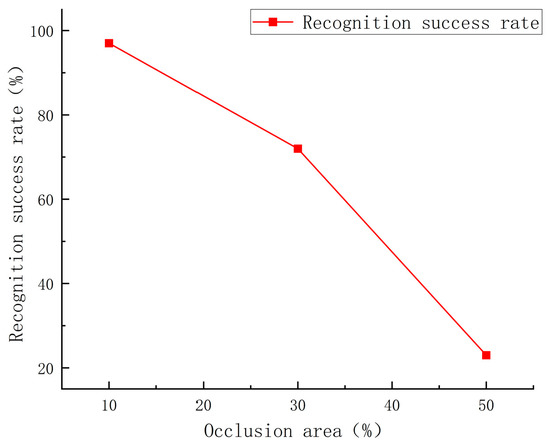
Figure 17.
Apriltag occlusion recognition success rate.
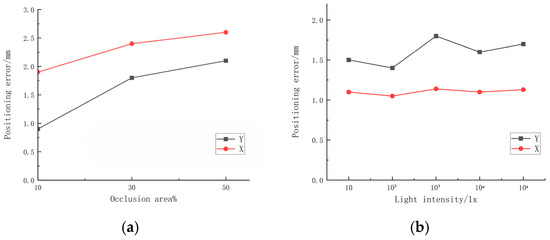
Figure 18.
Apriltag occlusion illumination experiment results. (a) Positioning error with changes in occlusion. (b) Positioning error with changes in light intensity.
The illumination condition results are shown in Figure 18b. In the illumination interference experiments, the positioning errors of the system in the XY plane are less than 2.0 mm, the average error in the X direction is 1.1 mm, and the average error in the Y direction is 1.6 mm. The change in light intensity has little effect on the positioning errors in the X and Y directions. The errors in the X direction are basically flat, and the errors in the Y direction fluctuate slightly, with the maximum fluctuation value at about 0.5 mm.
Apriltag distance and interference condition results are shown in Figure 19. It can be seen from Figure 19a that, in the case of an interference background, the positioning errors of the system in the XY plane are less than 1.0 mm, in which the average error in the X direction is 0.7 mm, and the average error in the Y direction is 0.4 mm. In addition, the experiments show that the interference background has little effect on the positioning errors in the X and Y directions. In addition to the background interference, in the outdoor environment, the target is usually moved due to vibrations, wind load, and other factors, so that the working distance is no longer a fixed value. In this case, the camera depth of field and system stability have high requirements. Therefore, various working conditions of the target in the range of 0.5 m before and after the focal plane of the camera were tested. In the outdoor environment, the initial working distance of 1.5 m is selected to focus the camera, and then the working distance is adjusted to ±0.5 m to verify the recognition and positioning of the camera in the ±0.5 m focus range. By changing the working distance, the lateral distance of the target, and the deflection angle, the recognition and positioning effect and the positioning error are shown in Figure 19b. The experimental results show that the system can effectively identify and locate in the range of ±0.5 m in the focal plane of the camera, and the positioning errors in the XY plane are less than 3.0 mm. The average error in the X direction is 1.5 mm, and the average error in the Y direction is 1.7 mm.
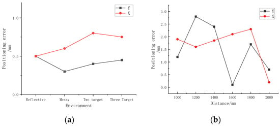
Figure 19.
Apriltag distance and interference experimental results diagram. (a) Positioning error with interference. (b) Positioning error with distance.
Under the recognition and positioning of the common and influential outdoor interference environment and working conditions, it can be seen from the experiments that the positioning errors in the XY plane in the outdoor interference environment are 1.36 mm and 1.44 mm, respectively, indicating that the Apriltag shows a high precision and quick recognition speed. In addition, after repeated experiments, the maximum fluctuation range of the positioning errors of the system are not more than 0.5 mm, indicating that the system is stable. In summary, Apriltag assisted positioning can achieve high-precision recognition and output positioning results in the case of outdoor light intensity changes, sudden occlusion, working distance changes, and interference background.
4. Discussion
It can be seen from the above experiments that the main factors affecting the positioning accuracy are the layout density and environmental conditions of Apriltags. In all the experiments, it can be seen that the density of Apriltag arrangement is directly related to the positioning accuracy. The denser the Apriltag arrangement, the higher the positioning accuracy. Under the same Apriltag layout density, the environmental factors also have a certain impact on the positioning accuracy. It can be seen from Table 2 that the positioning error of Scene1 is higher than that of Scene2 in general. This is because Scene1 is an open scene, and the feature points are sparse, so it is difficult to provide sufficient environmental information for mapping and positioning. For the orchard scene of Scene2, although its terrain is complex, due to the rich feature points (such as trunks, shrubs, etc.), it provides more reference information for the system, thereby improving the positioning accuracy. Therefore, the ‘complexity’ of the environment does not simply correspond to the positioning performance but needs to comprehensively consider multiple factors such as feature point density and ground flatness. From the X and Y direction errors of the experiments with different ds values, it can be seen that the overall errors in the Y direction are significantly greater than those in the X axis direction in Scenes 1 and 2, which strongly suggests that the system has a specific deviation source in the Y direction (such as inaccurate external parameter calibration). Considering that the joint calibration of IMU and LiDAR is inaccurate due to the small number of feature planes that can be extracted from the selected calibration scene [47], the scene is re-selected for calibration.
Considering the robustness and economic factors of the system in the specific environmental layout, for the areas with high precision requirements, such as nursery beds, we can use the distance of 3.0 m to arrange Apriltags. For the main channel with lower precision requirements, we can use the distance of 5.0 m to arrange Apriltags. And, in the equipment area and the edge area, we can use the distance of 10.0 m to arrange Apriltags.
However, there are still some shortcomings in the experiments. Due to limited time and conditions, we only carried out experiments in scenes similar to greenhouses or orchards. The validation of the proposed method needs more agricultural experiments and tests. We are planning to carry out long-term experiments on the actual corresponding scenarios in future research, observe the performance changes in the system during long-term operation, and discover and solve possible problems in time to ensure the reliability and practicability of the system.
In this design, we also consider the possibility of using UWB technology instead of GNSS as an absolute constraint. However, compared to UWB, Apriltag shows significant advantages, making it a more suitable choice for our application scenarios. First of all, Apriltag has a very low production cost and very simple system deployment, which has obvious advantages in large-scale applications and multi-scenario switching [48]. In addition, Apriltag has a wider adaptability to the environment and can maintain a stable performance both indoors and outdoors, even in greenhouses with complex and variable lighting conditions. This is mainly due to its strong robustness to changes in illumination and shooting angle, which is particularly important in challenging environments such as agricultural greenhouses. In terms of real-time performance, Apriltag also performs well. Its data update frequency is fast, and it can respond quickly to environmental changes, which is crucial for real-time positioning and navigation tasks. In contrast, although UWB technology can provide high-precision positioning in some scenarios, it is vulnerable to multipath effects and non-line-of-sight (NLOS) interference in complex environments, resulting in a reduced positioning accuracy. In addition, the data update frequency of UWB is relatively low, which makes it difficult to meet the real-time positioning requirements in a rapidly changing environment. In particular, the flexibility and ease of use of Apriltag are almost unparalleled. Its lightweight system design makes migration and reuse extremely convenient. It can be easily deployed and adjusted in different experimental environments and application scenarios, which greatly improves the efficiency of research and application. This convenience is particularly valuable in the ever-changing agricultural research environment and provides us with great convenience.
In practical applications, there are still some details that can be improved. Tags are susceptible to dirt, mud, water stains, and physical damage. Developing low-cost, self-cleaning or durable protective housings for tags is essential. Furthermore, investigating multi-spectral visual markers visible in specific wavelengths (e.g., near-infrared) could improve the reliability under varying lighting conditions and make the system less sensitive to visible-spectrum dirt and shadows. Additionally, for permanent installation in perennial crops (e.g., orchards, vineyards), the system must account for environmental changes. The software should incorporate a mechanism to detect and flag tags that may have been moved, rotated, or degraded over time, prompting recalibration or replacement. For fleet operations, a cloud-based infrastructure for storing and sharing the updated tag map among multiple robotic platforms would be necessary to ensure consistency and avoid repeated mapping procedures.
The system we designed has strong environmental adaptability and can be stably and accurately applied to various agricultural scenarios such as greenhouses and outdoor farmland. In the greenhouse planting environment and outdoor farmland, the traditional GNSS navigation scheme often fails due to signal occlusion and needs to be equipped with two sets of positioning equipment, which increases the cost and system complexity. Our system does not require hardware switching or a mode reset and can be seamlessly compatible with the greenhouse and farmland environment to achieve efficient autonomous operation and support the comprehensive planting management needs of modern agricultural parks.
5. Conclusions
In this paper, an agricultural autonomous positioning and navigation system based on Apriltag and LIO-SAM fusion positioning was designed. The moving platform was used to realize the mapping, straight turning, and obstacle avoidance of the autonomous positioning and navigation system in greenhouses, orchards, and other environments. The experimental analysis shows the following:
- (1)
- The average errors of the real-time map constructed by the Gmapping, LIO-SAM, and April-LIO-SAM algorithms in the greenhouse experimental scene were 0.599 m, 0.316 m, and 0.049 m, and the root mean square error was 0.630 m, 0.372 m, and 0.057 m, respectively. In the circumstances without a GNSS signal, the mapping accuracy of the April-LIO-SAM algorithm proposed in this paper is significantly better than other mapping algorithms. The navigation experiment results indicate that the average lateral deviation of autonomous navigation for mobile robots at different speeds is within the centimeter range, with the average heading deviation not exceeding 2.5°.
- (2)
- The positioning accuracy experiments of the autonomous positioning and navigation system were carried out in the greenhouse and orchard experimental environments. When the spacing is 3.0 m, 5.0 m, 7.0 m, and 10.0 m, the average deviations are 0.044 m, 0.057 m, 0.059 m, and 0.067 m in the X direction and 0.052 m, 0.060 m, 0.066 m, and 0.084 m in the Y direction in Scene1. In Scene2, the average deviations were 0.036 m, 0.039 m, 0.050 m, and 0.056 m in the X direction and 0.032 m, 0.040 m, 0.049 m, and 0.071 m in the Y direction. And the root mean square errors were 0.060, 0.069, 0.840, and 0.098 m in Scene1 and 0.059 m, 0.064 m, 0.079 m, and 0.082 m in Scene2. It can be seen that the autonomous positioning and navigation system designed in this paper still has a high accuracy in the greenhouse and orchard environments, meeting the operational requirements.
- (3)
- The Apriltag stability experiments were carried out with different occlusion and illumination conditions, background interference, and changing distance. The results show that the Apriltag recognition rate is high when the occlusion ratio is less than 30%. Apriltag positioning errors are within 3.0 mm under different interference conditions.
- (4)
- The autonomous navigation system designed in this study can effectively cope with the challenges of high similarity between rows in the greenhouse, poor GNSS signals, and uneven orchard terrain.
At present, the system implements basic navigation capabilities based on the basic move_base navigation function package in ROS. Future work will focus on improving navigation accuracy. Aiming at the problem of large amounts of calculation for traditional path planning algorithms in complex environments, it is planned to improve the heuristic function of the A* algorithm, introduce weight coefficients, and combine the Bezier curve to achieve trajectory smoothing. In order to improve the efficiency of the algorithm, we plan on reducing the computational and communication burden of the control platform so as to achieve smoother and more accurate motion in the greenhouse or orchard environment. At the same time, the stability of the Apriltag tags in the current design also needs to be improved. In the actual working environment, human activities or natural factors (such as wind blowing) may lead to label displacement, and plant growth may lead to label occlusion, which in turn affects positioning accuracy. Follow-up research will be devoted to solving these problems and improving the robustness and reliability of the system.
Author Contributions
Conceptualization and methodology, X.G.; software, H.G. and S.N.; methodology, H.G.; validation, X.G. and H.G.; formal analysis, X.G., Y.D. and H.G.; investigation, X.G., H.G. and S.N.; resources, X.G.; data curation, H.G. and Y.D.; writing—raw draft, H.G.; writing—review and editing, X.G. and Y.D.; visualization, H.G. and S.N.; supervision, X.G.; funding acquisition, X.G. All authors have read and agreed to the published version of the manuscript.
Funding
This work is funded by the Priority Academic Program Development of Jiangsu Higher Education Institutions (No. PAPD-2023-87).
Data Availability Statement
The original contributions presented in this study are included in the article. Further inquiries can be directed to the corresponding author.
Conflicts of Interest
The authors declare no conflicts of interest.
Abbreviations
The following abbreviations are used in this manuscript:
| GNSS | Global Navigation Satellite System |
| LIO-SAM | Tightly Coupled LiDAR Inertial Odometry via Smoothing and Mapping |
| IMU | Inertial Measurement Unit |
| SLAM | Simultaneous Localization and Mapping |
| LiDAR | Light Detection and Ranging |
| UWB | Ultra-Wide Band |
| AMCL | Adaptive Monte Carlo Localization |
| RANSAC | Random Sample Consensus |
| RTK | Real-Time Kinematic |
| RFID | Radio Frequency Identification |
| BLE | Bluetooth Low Energy |
| GPS | Global Positioning System |
Appendix A

Table A1.
Mobile chassis parameters.
Table A1.
Mobile chassis parameters.
| Appearance Size (Length × Width × Height) | 830 × 620 × 370 mm |
| Weight | 55 kg |
| Speed | 0–2.2 m/s |
| Steering characteristics | Differential drive |
| Drive battery specifications | 24 V 30 ah |
| Maximum climbing slope | 25° |
| Remote control communication frequency | 2.4 G/Hz |
| Remote control distance | 0–150 m |
| Rated self-rotating load | 75 kg |

Table A2.
Servo motor, encoder, and reducer related parameters.
Table A2.
Servo motor, encoder, and reducer related parameters.
| Motor rated power | 250 W |
| Encoder accuracy | 0.09° |
| Reducer speed ratio | 29.17 |
References
- Ma, Z.; Yang, S.; Li, J.; Qi, J. Research on SLAM Localization Algorithm for Orchard Dynamic Vision Based on YOLOD-SLAM2. Agriculture 2024, 9, 1622. [Google Scholar] [CrossRef]
- Guan, C.; Zhao, W.; Xu, B.; Cui, Z.; Yang, Y.; Gong, Y. Design and Experiment of Electric Uncrewed Transport Vehicle for Solanaceous Vegetables in Greenhouse. Agriculture 2025, 15, 118. [Google Scholar] [CrossRef]
- Zhang, E.; Ma, Z.; Geng, C.; Li, W. Control system for automatic track transferring of greenhouse hanging sprayer. J. China Agric. Univ. 2013, 18, 170–174. Available online: http://zgnydxxb.ijournals.cn/zgnydxxb/ch/reader/view_abstract.aspx?file_no=20130625&flag=1 (accessed on 18 September 2025).
- Aranda, F.J.; Parralejo, F.; Álvarez, F.J.; Paredes, J.A. Performance analysis of fingerprinting indoor positioning methods with BLE. Expert Syst. Appl. 2022, 202, 117095. [Google Scholar] [CrossRef]
- Abdullah, A.; Aziz, O.A.; Rashid, R.A.; Haris, M.; Sarijari, M.A. Robust and fast algorithm design for efficient Wi-Fi fingerprinting based indoor positioning systems. J. King Saud Univ. Comput. Inf. Sci. 2023, 35, 101696. [Google Scholar] [CrossRef]
- Jin, G.; Liu, Q.; Yu, Y. Indoor Dynamic Positioning Method Exploiting Passive RFID System. IEEE Access 2024, 12, 170451–170458. [Google Scholar] [CrossRef]
- Xu, X.; Xu, D.; Zhang, T.; Zhao, H. In-Motion Coarse Alignment Method for SINS/GPS Using Position Loci. IEEE Sens. J. 2019, 19, 3930–3938. [Google Scholar] [CrossRef]
- Yao, Z.; Zhao, C.; Zhang, T. Agricultural machinery automatic navigation technology. iScience 2024, 27, 108714. [Google Scholar] [CrossRef]
- Balaso, D.; Arima, S.; Ueka, Y.; Kono, M.; Nishina, H.; Kenji, H.; Takayama, K.; Takahashi, N. Development of a multi-operation system for intelligent greenhouses. IFAC Proc. Vol. 2013, 46, 158–178. [Google Scholar] [CrossRef]
- Jiang, S.; Qi, P.; Han, L.; Liu, L.; Li, Y.; Huang, Z.; Liu, Y.; He, X. Navigation system for orchard spraying robot based on 3D LiDAR SLAM with NDT_ICP point cloud registration. Comput. Electron. Agric. 2024, 220, 108870. [Google Scholar] [CrossRef]
- Bagagiolo, G.; Matranga, G.; Cavallo, E.; Pampuro, N. Greenhouse Robots: Ultimate Solutions to Improve Automation in Protected Cropping Systems—A Review. Sustainability 2022, 14, 6436. [Google Scholar] [CrossRef]
- Chen, X.; Wang, S.; Zhang, B.; Luo, L. Multi-feature fusion tree trunk detection and orchard mobile robot localization using camera/ultrasonic sensors. Comput. Electron. Agric. 2018, 147, 91–108. [Google Scholar] [CrossRef]
- Long, Z.; Xiang, Y.; Lei, X.; Li, Y.; Hu, Z.; Dai, X. Integrated indoor positioning system of greenhouse robot based on UWB/IMU/ODOM/LIDAR. Sensors 2022, 22, 4819. [Google Scholar] [CrossRef]
- Niu, Z.; Yang, H.; Zhou, L.; Farag Taha, M.; He, Y.; Qiu, Z. Deep learning-based ranging error mitigation method for UWB localization system in greenhouse. Comput. Electron. Agric. 2023, 205, 107573. [Google Scholar] [CrossRef]
- Li, Y.; Shen, H.; Fu, Y.; Wang, K. A method of dense point cloud SLAM based on improved YOLOV8 and fused with ORB-SLAM3 to cope with dynamic environments. Expert Syst. Appl. 2024, 255, 124918. [Google Scholar] [CrossRef]
- Lv, X.; Zhang, X.; Gao, H.; He, T.; Lv, Z.; Zhang, L. When crops meet machine vision: A review and development framework for a low-cost nondestructive online monitoring technology in agricultural production. Agric. Commun. 2024, 2, 100029. [Google Scholar] [CrossRef]
- Khan, M.S.U.; Ahmed, T.; Chen, H. A Review of SLAM Techniques for Agricultural Robotics: Challenges, Architectures, and Future Directions. In Proceedings of the 2025 IEEE 15th International Conference on CYBER Technology in Automation, Control, and Intelligent Systems (CYBER), Shanghai, China, 15–18 July 2025; pp. 598–603. [Google Scholar] [CrossRef]
- Alhmiedat, T.; M Marei, A.; Messoudi, W. A SLAM-Based Localization and Navigation System for Social Robots: The Pepper Robot Case. Machines 2023, 11, 158. [Google Scholar] [CrossRef]
- Jiang, A.; Ahamed, T. Development of an autonomous navigation system for orchard spraying robots integrating a thermal camera and LiDAR using a deep learning algorithm under low- and no-light conditions. Comput. Electron. Agric. 2025, 235, 110359. [Google Scholar] [CrossRef]
- Baltazar, J.D.A.; Coelho, A.L.D.F.; Valente, D.S.M.; Queiroz, D.M.D.; Villar, F.M.D.M. Development of a Robotic Platform with Autonomous Navigation System for Agriculture. AgriEngineering 2024, 6, 3362–3374. [Google Scholar] [CrossRef]
- Olson, E. AprilTag: A robust and flexible visual fiducial system. In Proceedings of the 2011 IEEE International Conference on Robotics and Automation, Shanghai, China, 9–13 May 2011; pp. 3400–3407. [Google Scholar] [CrossRef]
- Kalaitzakis, M.; Cain, B.; Carroll, S.; Ambrosi, A.; Whitehead, C.; Vitzilaios, N. Fiducial Markers for Pose Estimation: Overview, Applications and Experimental Comparison of the ARTag, AprilTag, ArUco and STag Markers. J. Intell. Robot. Syst. 2021, 101, 71. [Google Scholar] [CrossRef]
- Garrido-Jurado, S.; Muñoz-Salinas, R.; Madrid-Cuevas, F.J.; Medina-Carnicer, R. Generation of fiducial marker dictionaries using Mixed Integer Linear Programming. Pattern Recognit. 2016, 51, 481–491. [Google Scholar] [CrossRef]
- Zhang, W.; Gong, L.; Huang, S.; Wu, S.; Liu, C. Factor graph-based high-precision visual positioning for agricultural robots with fiducial markers. Comput. Electron. Agric. 2022, 201, 107295. [Google Scholar] [CrossRef]
- Chen, J.; Qiang, H.; Wu, J.; Xu, G.; Wang, Z.; Liu, X. Extracting the navigationpath of a tomato-cucumber greenhouse robot based on amedian point hough transform. Comput. Electron. Agric. 2020, 174, 105472. [Google Scholar] [CrossRef]
- Tan, H.; Zhao, X.; Fu, H.; Yang, M.; Zhai, C. A novel fusion positioning navigation system for greenhouse strawberry spraying robot using LiDAR and ultrasonic tags. Agric. Commun. 2025, 3, 100087. [Google Scholar] [CrossRef]
- Nishimura, K.; Ishikawa, T.; Sasaki, H.; Kato, S. RAPLET: Demystifying Publish/Subscribe Latency for ROS Applications. In Proceedings of the 2021 IEEE 27th International Conference on Embedded and Real-Time Computing Systems and Applications (RTCSA), Houston, TX, USA, 18–20 August 2021; pp. 41–50. [Google Scholar] [CrossRef]
- Qin, T.; Li, P.; Shen, S. VINS-Mono: A Robust and Versatile Monocular Visual-Inertial State Estimator. IEEE Trans. Robot. 2018, 34, 1004–1020. [Google Scholar] [CrossRef]
- Lv, J.; Xu, J.; Hu, K.; Liu, Y.; Zuo, X. Targetless Calibration of LiDAR-IMU System Based on Continuous-time Batch Estimation. arXiv 2007, arXiv:2007.14759. [Google Scholar] [CrossRef]
- Gimpelj, J.; Semolič, M.; Munih, M.; Šlajpah, S.; Mihelj, M. Navigation of a Mobile Platform in a Greenhouse, in Advances in Service and Industrial Robotics. Mech. Mach. Sci. 2023, 135, 393–400. [Google Scholar] [CrossRef]
- Shan, T.; Englot, B.; Meyers, D.; Wang, W.; Ratti, C.; Rus, D. LIO-SAM: Tightly-coupled Lidar Inertial Odometry via Smoothing and Mapping. In Proceedings of the 2020 IEEE/RSJ International Conference on Intelligent Robots and Systems, Las Vegas, NV, USA, 24 October 2020–24 January 2021; pp. 5135–5142. [Google Scholar] [CrossRef]
- Xu, W.; Zhang, F. FAST-LIO: A Fast, Robust LiDAR-Inertial Odometry Package by Tightly-Coupled Iterated Kalman Filter. IEEE Robot. Autom. Lett. 2021, 6, 3317–3324. [Google Scholar] [CrossRef]
- Qin, T.; Pan, J.; Cao, S.; Shen, S. A General Optimization-based Framework for Local Odometry Estimation with Multiple Sensors. arXiv 2019, arXiv:1901.03638. [Google Scholar] [CrossRef]
- Huang, X.; Mei, G.; Zhang, J.; Abbas, R. A comprehensive survey on point cloud registration. arXiv 2021, arXiv:2103.02690. [Google Scholar] [CrossRef]
- Rusu, R.B.; Cousins, S. 3D is here: Point Cloud Library (PCL). In Proceedings of the 2011 IEEE International Conference on Robotics and Automation, Shanghai, China, 9–13 May 2011; pp. 1–4. [Google Scholar] [CrossRef]
- Zhang, J.; Singh, S. Real-Time. In Robotics: Science and Systems X; Robotics: Science and Systems Foundation: College Station, TX, USA, 2014; Volume 12. [Google Scholar] [CrossRef]
- Hong, L.; Han, L.; Liu, H. Unstructured Road Slope Recognition Based on Improved RANSAC Algorithm. In Proceedings of the 2023 5th International Conference on Communications, Information System and Computer Engineering (CISCE), Guangzhou, China, 14–16 April 2023; pp. 322–325. [Google Scholar] [CrossRef]
- Wang, Y.; Zheng, J.; Xu, Q.-Z.; Li, B.; Hu, H.-M. An improved RANSAC based on the scale variation homogeneity. J. Vis. Commun. Image Represent. 2016, 40, 751–764. [Google Scholar] [CrossRef]
- Hartley, R.; Jadidi, M.G.; Gan, L.; Huang, J.-K.; Grizzle, J.W.; Eustice, R.M. Hybrid Contact Preintegration for Visual-Inertial-Contact State Estimation Using Factor Graphs. In Proceedings of the 2018 IEEE/RSJ International Conference on Intelligent Robots and Systems (IROS), Madrid, Spain, 1–5 October 2018; pp. 3783–3790. [Google Scholar] [CrossRef]
- Barfoot, T.D. State Estimation for Robotics; Cambridge University Press: Cambridge, UK, 2017; pp. 31–52. [Google Scholar]
- Nisar, B.; Foehn, P.; Falanga, D.; Scaramuzza, D. VIMO: Simultaneous Visual Inertial Model-Based Odometry and Force Estimation. IEEE Robot. Autom. Lett. 2019, 4, 2785–2792. [Google Scholar] [CrossRef]
- Yu, S.; Wu, T. Application research of GPS-RTK combined with total station in cadastral surveying in mountainous areas. Heilongjiang Hydraul. Sci. Technol. 2018, 46, 135–136. Available online: https://www.cnki.com.cn/Article/CJFDTotal-HSKJ201809045.htm (accessed on 18 September 2025).
- Moore, T.; Stouch, D. A Generalized Extended Kalman Filter Implementation for The Robot Operating System. Intell. Auton. Syst. 2016, 13, 335–348. [Google Scholar]
- Huang, Y.-H.; Lin, C.-T. Indoor Localization Method for a Mobile Robot Using LiDAR and a Dual Apriltag. Electronics 2023, 12, 1023. [Google Scholar] [CrossRef]
- Chen, J.; Zhu, F.; Guan, Z.; Zhu, Y.; Shi, H.; Cheng, K. Development of a combined harvester navigation control system based on visual simultaneous localization and mapping-inertial guidance fusion. J. Agric. Eng. 2024, 7, 7–13. [Google Scholar] [CrossRef]
- Li, B.; Huang, X.; Cai, J.; Ma, F. LB-LIOSAM: An improved mapping and localization method with loop detection. Ind. Robot Int. J. Robot. Res. Appl. 2025, 52, 381–390. [Google Scholar] [CrossRef]
- Pedersini, F. Simple Calibration of Three-Axis Accelerometers with Freely Rotating Vertical Bench. Sensors 2025, 25, 3998. [Google Scholar] [CrossRef] [PubMed]
- Zhou, J.; Mao, K.; Wang, R.; He, T.; Liang, H. Autonomous Navigation Method for UAV Based on the Fusion of Laser SLAM and Apriltag. J. Phys. Conf. Ser. 2025, 3012, 012002. [Google Scholar] [CrossRef]
Disclaimer/Publisher’s Note: The statements, opinions and data contained in all publications are solely those of the individual author(s) and contributor(s) and not of MDPI and/or the editor(s). MDPI and/or the editor(s) disclaim responsibility for any injury to people or property resulting from any ideas, methods, instructions or products referred to in the content. |
© 2025 by the authors. Licensee MDPI, Basel, Switzerland. This article is an open access article distributed under the terms and conditions of the Creative Commons Attribution (CC BY) license (https://creativecommons.org/licenses/by/4.0/).