Research on Spatiotemporal Combination Optimization of Remote Sensing Mapping of Farmland Soil Organic Matter Considering Annual Variability

Abstract

Soil organic matter (SOM) is a key indicator of cropland quality and carbon cycling. Accurate SOM mapping is essential for sustainable soil management and carbon sink assessment. This study investigated the effects of interannual climatic variability on SOM prediction using remote sensing and machine learning. Youyi Farm in the Sanjiang Plain, Heilongjiang Province, was selected as the study area, covering three representative years: 2019 (flood), 2020 (normal), and 2021 (drought). Based on multi-temporal Sentinel-2 imagery and environmental covariates, Random Forest models were used to evaluate single- and dual-period combinations. Results showed that combining bare-soil and crop-season images consistently improved accuracy, with optimal combinations varying by year (R² = 0.544–0.609). Incorporating temperature, precipitation, and elevation enhanced model performance, particularly temperature, which contributed most to prediction accuracy. Feature selection further improved model stability and generalization. Spatially, SOM showed a pattern of higher values in the northeast and lower in the central region, shaped by topography and cultivation. This study innovatively integrates interannual climatic variability with remote sensing temporal combination and feature selection, constructing a climate-adaptive SOM mapping framework and providing new insights for accurate inversion of cropland SOM under extreme climates, highlights the importance of multi-temporal imagery, environmental factors, and feature selection for robust SOM mapping under different climatic conditions, providing technical support for long-term cropland quality monitoring.

1. Introduction

Soil organic matter (SOM) is one of the most critical components of cropland soils and plays a fundamental role in maintaining soil health and ensuring sustainable agricultural development [1]. In the context of the global carbon cycle, SOM constitutes an essential part of the terrestrial carbon pool [2] and plays a key role in carbon sequestration and greenhouse gas balance [3]. Changes in SOM not only affect carbon cycling dynamics within agricultural systems but also directly influence global climate regulation mechanisms [4]. Regarding soil fertility, the functional mechanisms of SOM are complex and multifaceted. On one hand, SOM can enhance the retention of nutrients such as nitrogen, phosphorus, and potassium through adsorption and complexation processes [5]. On the other hand, it improves soil aggregate structure, thereby enhancing soil aeration and water-holding capacity [6]. However, in recent years, long-term cultivation has led to severe SOM degradation [7], and the consequent reduction in SOM content may accelerate soil degradation and pose a threat to food security [8]. Therefore, predicting the spatial distribution of SOM is crucial for land conservation and sustainable utilization.

Over the past decades, with the continuous development of remote sensing technology and machine learning algorithms, digital soil mapping (DSM) has been widely applied in the prediction of soil properties [9]. Remote sensing offers advantages such as wide spatial coverage, efficient data acquisition, and high temporal resolution [10], effectively overcoming the high costs and limited representativeness associated with traditional soil sampling. Consequently, it has gradually become a core technical approach for monitoring and assessing cropland SOM, providing abundant data sources for SOM mapping [11]. Meanwhile, machine learning algorithms can capture the complex nonlinear relationships between remote sensing data and soil organic matter, thereby improving mapping accuracy [12]. With the development of remote sensing technology and the introduction of machine learning methods, the accuracy and efficiency of spatial prediction of SOM have been significantly improved [13]. Traditional statistical methods often rely on linear assumptions during modeling, making it difficult to fully capture the complex nonlinear relationships among soil, climate, topography, and vegetation [13]. In contrast, machine learning approaches, such as Random Forest (RF), Gradient Boosting Trees (XGBoost), and Cubist, can handle high-dimensional, multi-source heterogeneous data and automatically identify nonlinear and interactive effects among variables, thus being widely applied in DSM [14]. Especially when estimating SOM using remote sensing data, machine learning models can fully exploit multi-temporal and multi-spectral information by integrating bare-soil and crop-season imagery with meteorological and topographic factors, thereby improving prediction accuracy and spatial generalization [15]. In addition, machine learning methods exhibit strong robustness, accommodating variations in data quality and sample distribution under different climatic conditions, enabling stable performance across drought, flood, and normal years. Furthermore, with the increasing availability of high-resolution remote sensing imagery and multi-source data, combining machine learning models with feature selection and data fusion strategies can effectively reduce redundant variables and enhance model interpretability. Collectively, integrating remote sensing imagery with machine learning methods allows for accurate estimation and spatial mapping of SOM in black soil regions under varying climatic conditions, providing a scientific basis for black soil conservation and sustainable agricultural development.

In this application process, the performance of remote sensing imagery in soil monitoring is constrained by surface cover conditions [16]. Images acquired during the bare-soil period can often provide more direct spectral information of the soil, thereby offering distinct advantages for SOM mapping [17]. However, imagery from the crop-growing season should not be overlooked. Vegetation growth is closely related to soil nutrient content and can indirectly reflect SOM levels [18]. Therefore, bare-soil and crop-season images are complementary. In recent years, an increasing number of studies have shown that the judicious combination of these two temporal datasets can significantly improve the accuracy of soil property predictions [19]. Nevertheless, the applicability and effectiveness of such combinations may vary across regions and climatic conditions, and scientifically selecting the appropriate temporal combination remains a key challenge in remote sensing-based soil mapping [20].

Climatic conditions are a key external factor influencing the spectral signals of soil and vegetation in remote sensing imagery [21]. Variations in precipitation and temperature can modify soil moisture, vegetation cover, and crop growth dynamics, thereby altering the spectral responses of both soil and vegetation [22]. In flood years, excessive precipitation increases soil saturation and promotes vigorous crop growth, resulting in a marked reduction in bare-soil areas. Under these conditions, soil reflectance is often masked by high moisture levels and dense vegetation cover, limiting the usability of bare-soil period imagery [23]. In such cases, crop-season imagery may play a more important role, as the growth state of crops directly reflects soil nutrient and moisture conditions, thereby indirectly providing information for SOM estimation [24].Conversely, in drought years, insufficient precipitation and dry soils suppress crop growth, resulting in relatively larger bare-soil areas. Under these conditions, bare-soil period imagery can more clearly capture soil spectral characteristics [25]. However, arid conditions may alter surface soil structure and reflectance, and without correction for moisture conditions, this can introduce biases in SOM estimation [26]. In normal years, moderate soil moisture and temperature conditions maintain a balance between crop cover and bare-soil exposure, allowing soil information to be obtained while vegetation signals indirectly reflect soil properties, thereby stabilizing the accuracy of image combinations. Overall, interannual climatic variability significantly modulates the spectral responses of soil and vegetation, potentially leading to differences in the optimal temporal combination strategies under different climatic conditions. Therefore, investigating the variation patterns of image features under various climatic scenarios and exploring optimal image combinations for flood, drought, and normal years are crucial for improving SOM mapping accuracy and enhancing the robustness of predictive models.

In summary, although DSM has made considerable progress across various regions and scales, existing studies have rarely systematically considered the effects of interannual climatic variability on the accuracy of remote sensing-based SOM predictions. In particular, the adaptability and functional mechanisms of multi-temporal image combination strategies, environmental covariates, and feature selection under different climatic conditions remain unclear in typical farmland ecosystems. This research gap can be attributed to three key constraints: First, historical DSM studies have often prioritized spatial variability of SOM while treating temporal dynamics as a secondary factor—many studies focus on single-year or short-term datasets, assuming relatively stable climatic conditions over the study period, which overlooks the modulatory role of interannual climate fluctuations on soil–vegetation spectral responses. Second, data availability and consistency pose practical challenges: Long-term, high-quality remote sensing datasets are often scarce, especially for regions with frequent extreme weather; meanwhile, matching multi-year remote sensing data with synchronous in situ SOM samples requires substantial labor and resource investment, which limits large-scale systematic investigations. Third, methodological limitations in integrating climate variability: Traditional machine learning models for DSM are often optimized for specific climatic conditions and lack adaptive frameworks to quantify how interannual changes in temperature/precipitation alter the predictive power of remote sensing features. To address this gap, this study focused on Youyi Farm in the Sanjiang Plain and selected three representative climatic years: 2019 (flood year), 2020 (normal year), and 2021 (drought year). By integrating multi-temporal Sentinel-2 imagery, environmental factors, and a RF model, we systematically evaluated the mapping performance of single-period and dual-period image combinations, examined the contributions of environmental covariates and feature selection to model accuracy and stability, and revealed the spatial distribution patterns of cropland SOM under different climatic conditions. Notably, this study innovatively links interannual climatic variability to the optimization of remote sensing temporal combinations for SOM mapping, avoiding the “one-size-fits-all” limitation of traditional fixed-period strategies. It also proposes an RF-RFE feature selection framework tailored to complex climatic scenarios, which enhances the robustness of SOM prediction by adaptively screening key features across flood, normal, and drought years. This study aims to refine the methodological framework for SOM mapping under complex climatic scenarios, providing both theoretical guidance and practical references for multi-year cropland quality monitoring, agricultural management, and carbon sink assessment.

2. Materials and Methods

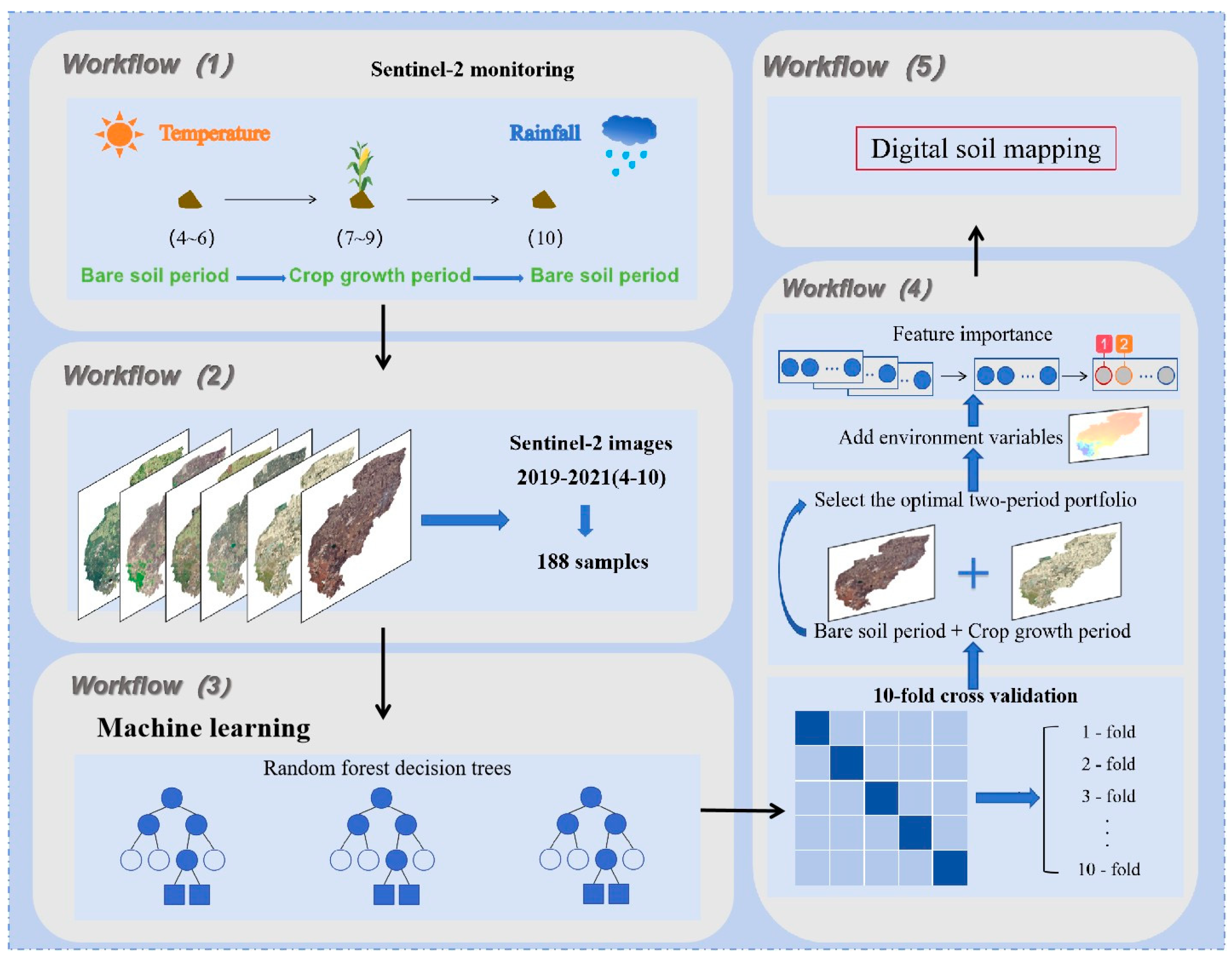
The basic flowchart of this study is shown in Figure 1.

2.1. Study Area

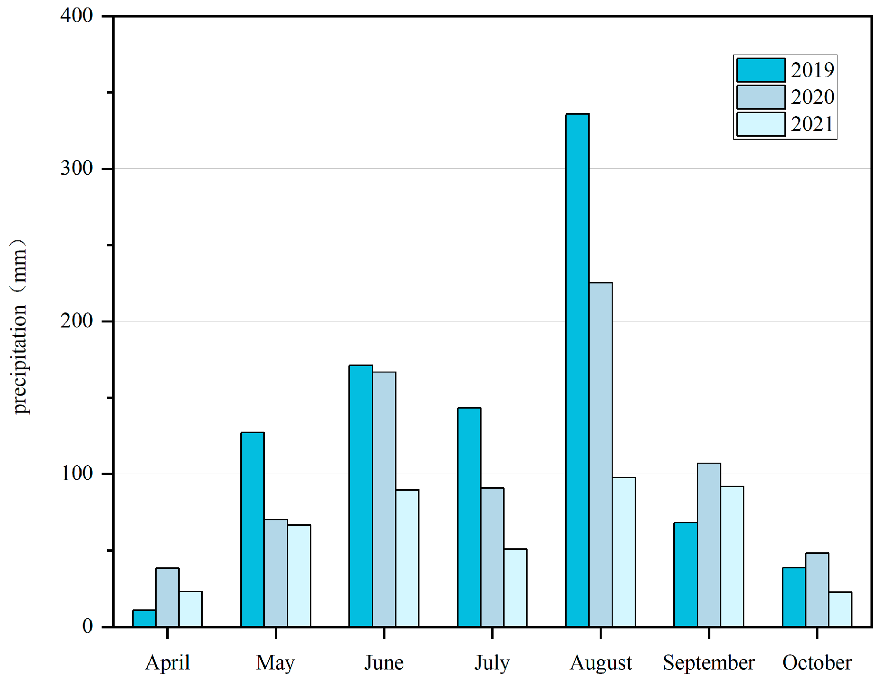
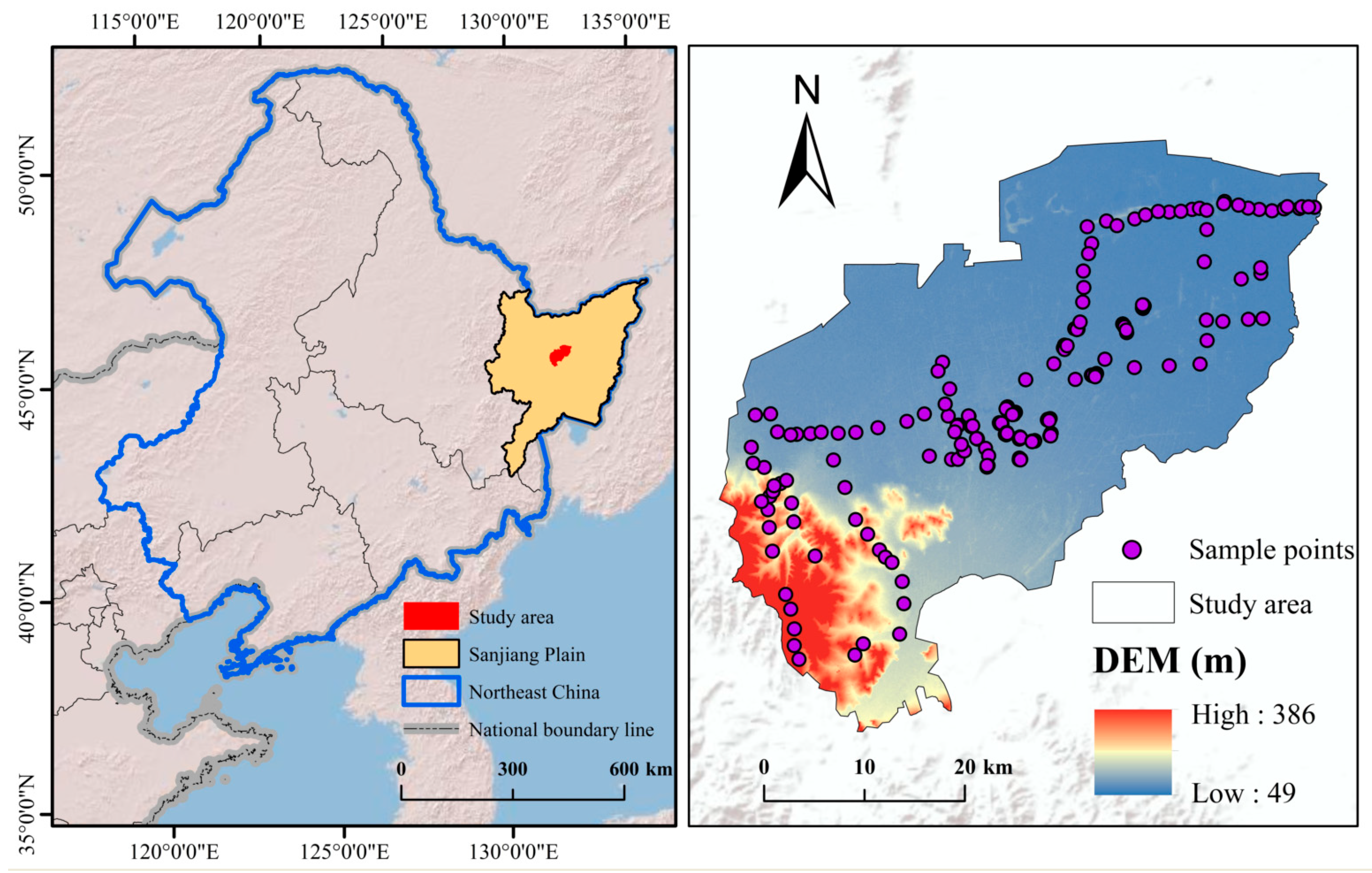
Youyi Farm is located in the central part of the Sanjiang Plain in Northeast China (131°15′–131°27′ E, 46°28′–46°59′ N) and is under the jurisdiction of Youyi County, of which the cultivated land area amounts to 1293.9 square kilometers (Figure 2). The region where Youyi Farm is situated has a temperate continental monsoon climate, featuring warm and rainy summers as well as cold and dry winters [27]. According to climatic records, the area has a long-term average annual precipitation of approximately 587.16 mm and a mean annual temperature of 3.1 °C (Figure 3). The terrain of the study area is generally flat with slight undulations. During the study period (2019–2021), Youyi Farm implemented standardized agricultural management under the regional “Black Soil Conservation Program,” resulting in a basically consistent agricultural practice model across years. The local crops are mainly soybeans, corn, and rice, which are harvested once a year. The dominant soil types are black soil and dark-brown soil, both widely distributed in Northeast China and exhibiting high fertility and representativeness. Black soil is rich in organic matter and highly fertile, representing an important high-quality cropland resource. Although dark-brown soil has slightly lower organic matter content, it possesses good structural properties and strong water- and nutrient-retention capacities, making it suitable for agricultural cultivation.

2.2. Data Sources

Remote sensing data were obtained from the Google Earth Engine (GEE) platform, comprising 20 Sentinel-2 surface reflectance scenes acquired from April to October during 2019–2021 (no imagery was available for July 2019), each with cloud coverage less than 5%. Using ArcGIS 10.8, suitable scenes were mosaicked into a single composite image via the “Mosaic to New Raster” tool. To maintain spatial consistency with other environmental variables, the mosaicked imagery was reprojected to the WGS_1984_UTM_Zone_52N coordinate system and resampled to a 10 m spatial resolution using the “Project Raster” tool. Bands that showed weak correlations with SOM or were mainly used for atmospheric correction (B1 and B10) were removed, retaining ten spectral bands (B2–B8A, B11, and B12) for subsequent analysis (

Table 1. Band details of the selected Sentinel-2 image [28].

Band Name	Description	Wavelength (nm)	Resolution (m)
B2	Blue	490	10
B3	Green	560	10
B4	Red	665	10
B5	Red Edge 1	705	20
B6	Red Edge 2	740	20
B7	Red Edge 3	783	20
B8	NIR	833	10
B8A	Red Edge 4	865	20
B11	SWIR 1	1610	20
B12	SWIR 2	2190	20

) [28].

A total of 188 soil samples were collected across the study area using a stratified random sampling approach, which comprehensively considered factors such as soil type, crop distribution, land-use patterns, and accessibility to ensure spatial representativeness. Field sampling was conducted in April 2021, during the early spring season before crop emergence, to minimize vegetation interference. At each sampling site, a 5 m × 5 m plot was established, and five subsamples were taken from the four corners and the center of the plot at a depth of 0–20 cm using a stainless-steel auger. The subsamples were thoroughly mixed to form a composite sample, yielding approximately 2 kg of soil per site. The precise geographic coordinates of each sampling point were recorded using a handheld GPS device to facilitate spatial modeling. All soil samples were air-dried, gently crushed, and sieved through a 2 mm mesh to remove coarse debris. Soil organic carbon SOC content was determined using the potassium dichromate oxidation (Walkley–Black) method. SOC values were then converted to SOM using the conventional conversion factor of 1.724 (SOM (g·kg⁻¹) = SOC (g·kg⁻¹) × 1.724) [28,29]. Next, using the centroid-based matching method in ArcGIS 10.8, each sampling point is spatially connected to the corresponding pixel in the Sentinel-2 image. The reflectance value of that pixel for each band was extracted and assigned to the corresponding SOM sample. This one-to-one matching method ensures spatial consistency between field observations and raster data, minimizing positional uncertainty. Since SOM changes are negligible over short timescales under stable management and climatic conditions, the 2021 samples were used for modeling SOM over a three-year period, providing a representative dataset for the study. The sampling point information for this paper is shown in

Table 2. Sampling point information.

Soil Indicators	Average Value	Minimum Value	Median	Maximum Value	Standard Deviation	Coefficient of Variation
SOM	3.92	0.48	3.59	9.91	1.41	35.93%

.

Environmental variables were derived from the Google Earth Engine (GEE), including the digital elevation model (DEM), average annual precipitation, and annual average temperature of the study area. Additionally, slope data were extracted from the DEM using ArcGIS 10.8 (

Table 3. Environmental variables information.

Environmental Variables	Unit	Data Type	Spatial Resolution
Annual Average Temperature	°C	raster	10 m
Average Annual Precipitation	mm	raster	10 m
DEM	m	raster	10 m
Slope	°	raster	10 m

). These variables capture the natural geographic conditions of the study area and serve as auxiliary information for SOM mapping [28].

2.3. Methodology

2.3.1. Multi-Temporal Combination Design

To evaluate the contribution of remote sensing information at different time scales to soil organic matter (SOM) prediction, we designed two modeling strategies:

Single-period modeling: Independent models were constructed using monthly imagery from April to October each year to assess the predictive power of each period and identify key time windows. Except for July 2019 (due to the lack of suitable imagery), one cloud-free Sentinel-2 image (cloud cover < 5%) was selected for analysis each month. This ensured consistency in temporal coverage over the three-year study period and minimized the impact of cloud contamination.

Two-period modeling: Building upon the single-period approach, imagery from two key months was fused, focusing on bare soil and representative periods of the crop-growing season. This strategy aimed to explore the improvement in model accuracy and interannual performance differences resulting from image fusion.

2.3.2. Feature Extraction and Preprocessing

Spectral features were extracted from preprocessed Sentinel-2 imagery to construct a feature dataset. The selected features included ten original spectral bands (B2–B8A, B11, and B12). Furthermore, the slope was calculated based on the DEM using ArcGIS 10.8’s “Slope” tool. Average temperature and precipitation datasets were obtained from the National Earth System Science Data Center (http://www.geodata.cn/) and the National Tibetan Plateau Data Center (https://data.tpdc.ac.cn/), respectively [28]. After processing with ArcGIS 10.8, annual average temperature and precipitation were calculated. Finally, after concatenation with sample points, the combination of spectral features, temperature, precipitation, and topographic features constituted the final input dataset for SOM prediction.

2.3.3. Feature Selection

Recursive Feature Elimination (RFE) is a feature selection method based on support vector machines [30]. The subsequently introduced Random Forest-based variant (RF-RFE) has gained widespread adoption in fields such as remote sensing due to its enhanced robustness and superior accuracy in handling complex data relationships. This method iteratively evaluates the contribution of each feature to model performance. In each iteration, a RF model is constructed using the current feature subset, and model performance is assessed using the coefficient of determination (R²) and root mean square error (RMSE) as metrics. Features are then ranked by importance and progressively removed from lowest to highest importance until a predefined feature subset size is reached, achieving optimal predictive performance (i.e., maximum R² and minimum RMSE). To minimize bias during the feature selection process, the final feature subset is validated using 10-fold cross-validation, ensuring stability and generalizability of the selected features.

2.3.4. Modeling and Accuracy Assessment

RF is a non-parametric machine learning algorithm based on the ensemble learning paradigm, which has been widely applied to both classification and regression tasks due to its high predictive accuracy, strong capability for nonlinear modeling, and robust fitting performance [31]. The RF model is constructed from an ensemble of regression trees, where each tree is generated using bootstrap sampling of the training dataset, and at each node split, a random subset of predictor variables is selected to determine the optimal partition. The final prediction is obtained by averaging the outputs of all individual trees, thereby enhancing model stability and generalization.

In this study, RF modeling was implemented in RStudio (R version 4.4.2). The algorithm was trained using the feature subset with the highest predictive relevance for soil organic matter inversion. Model optimization was conducted through k-fold cross-validation to ensure parameter robustness. The number of trees (ntree) was set to 1200, and the number of candidate variables at each split (mtry) was fixed at one-third of the total number of input features, in order to maximize prediction accuracy and model stability.

RF regression can be expressed as:

$$\widehat{y}={\displaystyle \frac{1}{T}}\sum _{t=1}^T{f}_t\left(x\right)$$

(1)

where $\widehat{y}$ is the final predicted value, $T$ is the number of regression trees, and ${\mathrm{f}}_{\mathrm{t}}\left(x\right)$ represents the prediction of the t tree for the input sample $x$.

In this study, a 10-fold cross-validation approach was employed to train and evaluate the performance of the SOM estimation model. The training dataset was randomly divided into 10 subsets. In each of the 10 folds, nine subsets were used for training and one subset for testing. The final estimate was obtained by averaging the results across all 10 folds. To assess model predictive performance, the coefficient of determination ($R^2$) and root mean square error ($RMSE$) were used as the primary evaluation metrics, calculated as follows:

$$R^2=1-{\displaystyle \frac{\sum _{i=1}^n{\left(y_i-{\widehat{y}}_i\right)}^2}{\sum _{i=1}^n{\left(y_i-{\overline{y}}_i\right)}^2}}$$

(2)

$$RMSE=\sqrt{{\displaystyle \frac{1}{n}}{\sum }_{i=1}^n{\left(y_i-{\widehat{y}}_i\right)}^2}$$

(3)

where $n$ is the total number of samples, $y_i$ is the observed value of sample $i$, ${\widehat{y}}_i$ i is the predicted value of sample $i$, and ${\overline{y}}_i$ is the mean of the observed values.

A well-performing model is typically characterized by a high $R^2$ value and a low $RMSE$. Specifically, an $R^2$ value approaching 1 indicates a good model fit, while a smaller $RMSE$ indicates that the deviation between predicted and observed values is low, reflecting higher predictive accuracy.

2.3.5. Modeling with Environmental Variables

Similarly, using the centroid matching method in ArcGIS 10.8, the coordinates of each sampling point were spatially matched with the corresponding 10 m resolution Sentinel-2 cell. The reflectance values of all bands of that cell, along with topographic variables (DEM, slope) and climate variables (annual mean precipitation and temperature) extracted within the same 10 m grid cell [32], were used as model inputs. This one-to-one matching method ensured spatial consistency between soil organic matter (SOM) measurements and environmental characteristics.

3. Results

Before presenting the modeling results, the configuration of predictor variables for each modeling scenario is summarized in

Table 4. Summary of predictor variables used in different modeling scenarios.

Model Type	Year (s)	Input Feature Categories	Number of Predictor Variables
Single-period	2019–2021	Spectral bands	10
Dual-period	2019–2021	Spectral bands (two months)	20
Dual-period + Environmental variables	2019–2021	Spectral + Environmental	24

. This table lists the categories and number of input features used in the single-period, dual-period, and integrated models.

3.1. Differences in Optimal Temporal Windows Under Different Climatic Years

Table 5. SOM prediction accuracy based on Sentinel-2 imagery for different months and years.

Date	R2	RMSE (g kg−1)	Date	R2	RMSE (g kg−1)
April 2019	0.383	1.103	August 2020	0.205	1.252
May 2019	0.426	1.064	September 2020	0.233	1.230
June 2019	0.311	1.166	October 2020	0.285	1.188
August 2019	0.260	1.208	April 2021	0.426	1.064
September 2019	0.198	1.258	May 2021	0.429	1.061
October 2019	0.157	1.290	June 2021	0.317	1.161
April 2020	0.355	1.128	July 2021	0.399	1.089
May 2020	0.507	0.986	August 2021	0.253	1.214
June 2020	0.510	0.983	September 2021	0.246	1.220
July 2020	0.438	1.053	October 2021	0.098	1.333

presents the single-period predictions of SOM based on Sentinel-2 imagery for 2019 (flood year), 2020 (normal year), and 2021 (drought year). Overall, climatic conditions had a significant impact on modeling accuracy.

In 2019, the model performed the poorest, with R² values ranging from 0.157 to 0.426 and RMSE from 1.064 to 1.290 g·kg⁻¹. The lowest accuracy was observed in October ($R^2$ = 0.157, RMSE = 1.290 g·kg⁻¹), likely due to excessive precipitation resulting in high soil moisture and enhanced vegetation masking effects. In 2021, although model accuracy was higher than in 2019, it remained lower than in 2020. May and April exhibited relatively better performance ($R^2$ = 0.429 and 0.426, respectively), while October showed a marked decline in accuracy ($R^2$ = 0.098, RMSE = 1.333 g·kg⁻¹). Under drought conditions, increased soil exposure facilitated the extraction of soil information, but the larger fluctuations in vegetation indices also introduced greater uncertainty. In contrast, 2020 exhibited the highest overall accuracy, with June and May achieving the best performance ($R^2$ = 0.510 and 0.507, respectively), benefiting from a relatively stable climate that strengthened the correlation between vegetation and SOM.

In summary, remote sensing-based modeling achieved the highest accuracy under normal climatic conditions. In contrast, during extreme years, interference from vegetation growth and soil moisture conditions significantly affected the remote sensing signals, leading to a decline in model performance.

3.2. Effect of Combining Bare Soil and Crop Growth Period Imagery

Table 6. SOM prediction accuracy based on dual-period Sentinel-2 imagery.

	Year/Month	2019		2020		2021
		R2	RMSE	R2	RMSE	R2	RMSE
Combination	4 + 7	-	-	0.476	1.017	0.468	1.025
	4 + 8	0.398	1.090	0.394	1.093	0.461	1.032
	4 + 9	0.388	1.099	0.400	1.088	0.448	1.044
	5 + 7	-	-	0.547	0.946	0.520	0.973
	5 + 8	0.437	1.054	0.512	0.981	0.480	1.013
	5 + 9	0.471	1.021	0.509	0.984	0.441	1.050
	6 + 7	-	-	0.563	0.928	0.410	1.079
	6 + 8	0.364	1.121	0.527	0.966	0.331	1.149
	6 + 9	0.384	1.102	0.525	0.968	0.373	1.113
	10 + 7	-	-	0.463	1.029	0.434	1.057
	10 + 8	0.287	1.186	0.285	1.188	0.286	1.187
	10 + 9	0.266	1.204	0.355	1.129	0.250	1.216

presents the modeling results based on dual-period imagery for different climatic years. Overall, the combination of bare-soil and crop growth period images outperformed single-period imagery.

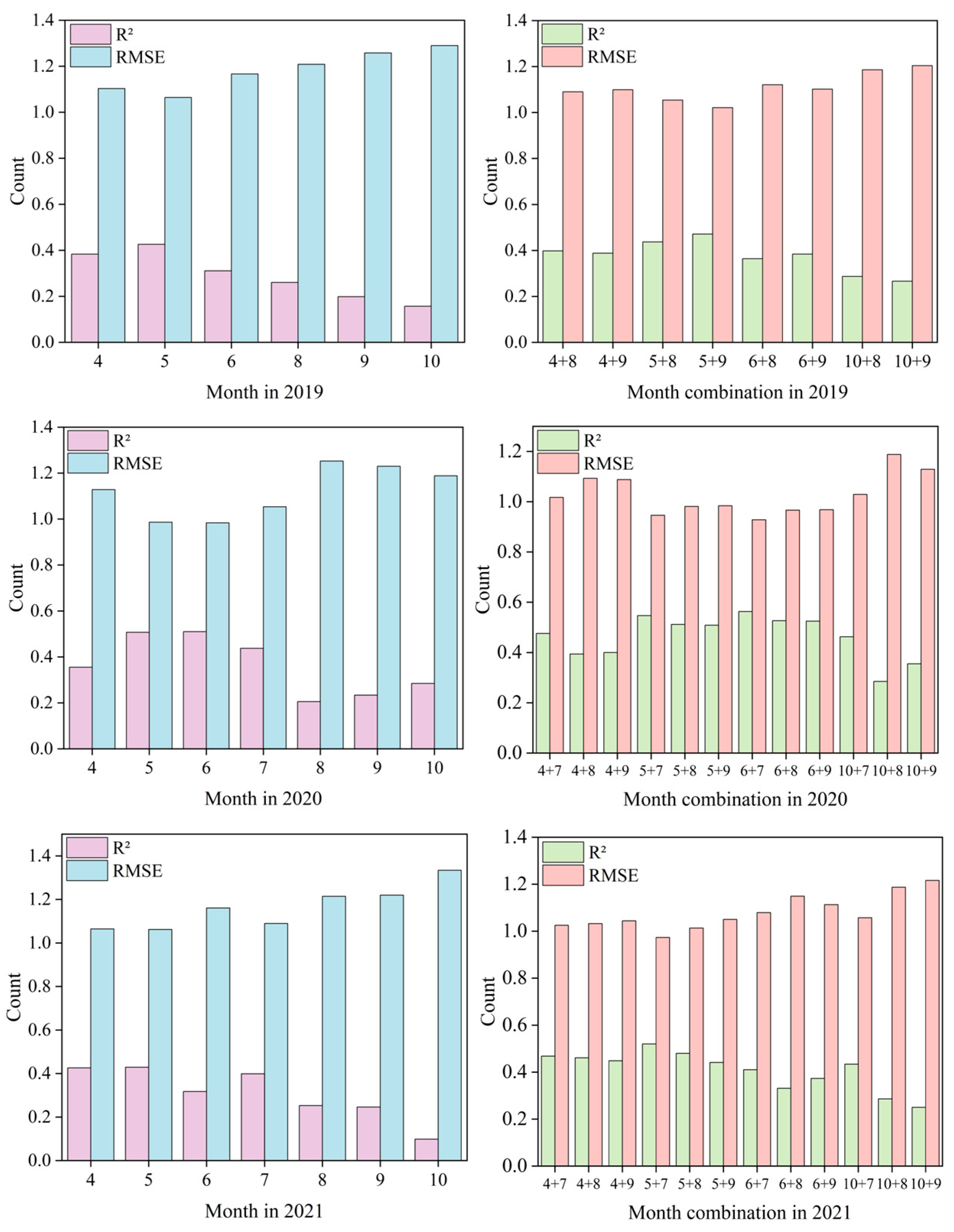
In 2019, the optimal combination was May and September ($R^2$ = 0.471, RMSE = 1.021 g·kg⁻¹); in 2020, June and July ($R^2$ = 0.563, RMSE = 0.928 g·kg⁻¹); and in 2021, May and July ($R^2$ = 0.520, RMSE = 0.973 g·kg⁻¹). All these optimal combinations included one bare-soil period and one crop growth period, indicating their complementary roles in SOM prediction: the bare-soil period captures soil background information, while the crop growth period provides information on vegetation growth.

The differences in optimal combinations across years also highlight the significant modulating effect of climate. In 2020, with vigorous crop growth, the crop growth period contributed more prominently, whereas in 2019 and 2021, the models relied more heavily on bare-soil imagery, likely due to unstable vegetation signals under flood and drought conditions. Notably, combinations involving October imagery consistently performed poorly, suggesting that post-harvest soil disturbance and crop residues negatively affected the remote sensing signals.

3.3. Improvement of Mapping Accuracy by Environmental Variables

Table 7. Comparison of SOM prediction accuracy for dual-period combinations before and after including environmental variables.

Year/Month		Combination		Combination + E
		R2	RMSE	R2	RMSE
2019	4 + 8	0.398	1.090	0.519	0.974
	4 + 9	0.388	1.099	0.531	0.962
	5 + 8	0.437	1.054	0.530	0.963
	5 + 9	0.471	1.021	0.537	0.956
	6 + 8	0.364	1.121	0.449	1.043
	6 + 9	0.384	1.102	0.466	1.026
	10 + 8	0.287	1.186	0.452	1.040
	10 + 9	0.266	1.204	0.452	1.040
2020	4 + 7	0.476	1.017	0.538	0.954
	4 + 8	0.394	1.093	0.528	0.965
	4 + 9	0.400	1.088	0.520	0.973
	5 + 7	0.547	0.946	0.588	0.901
	5 + 8	0.512	0.981	0.580	0.910
	5 + 9	0.509	0.984	0.575	0.915
	6 + 7	0.563	0.928	0.569	0.922
	6 + 8	0.527	0.966	0.566	0.926
	6 + 9	0.525	0.968	0.552	0.940
	10 + 7	0.463	1.029	0.512	0.981
	10 + 8	0.285	1.188	0.448	1.043
	10 + 9	0.355	1.129	0.491	1.003
2021	4 + 7	0.468	1.025	0.525	0.968
	4 + 8	0.461	1.032	0.549	0.944
	4 + 9	0.448	1.044	0.536	0.957
	5 + 7	0.520	0.973	0.566	0.926
	5 + 8	0.480	1.013	0.564	0.927
	5 + 9	0.441	1.050	0.547	0.946
	6 + 7	0.410	1.079	0.500	0.993
	6 + 8	0.331	1.149	0.502	0.992
	6 + 9	0.373	1.113	0.499	0.994
	10 + 7	0.434	1.057	0.508	0.985
	10 + 8	0.286	1.187	0.483	1.010
	10 + 9	0.250	1.216	0.477	1.016

compares the dual-period modeling results before and after the inclusion of environmental variables. The results indicate that environmental factors improved model accuracy across all three climatic years, with R² increasing by 0.05–0.10 and RMSE generally decreasing.

In 2019, the optimal combination (May + September) saw R² increase from 0.471 to 0.537, and RMSE decrease from 1.021 to 0.956 g·kg⁻¹. In 2020, the optimal combination (May + July) achieved an R² increase from 0.547 to 0.588 and RMSE decrease from 0.946 to 0.901 g·kg⁻¹. In 2021, the optimal combination (May + July) showed R² improvement from 0.520 to 0.566 and RMSE reduction from 0.973 to 0.926 g·kg⁻¹.

3.4. Differences in the Improvement of Mapping Accuracy Across Climatic Years by Feature Selection

Table 8. Comparison of SOM prediction accuracy for dual-period combinations before and after feature selection.

Year	Month	Combination + E		Combination + E + RFE
		R2	RMSE	R2	RMSE
2019	5 + 9	0.537	0.956	0.544	0.949
2020	5 + 7	0.588	0.901	0.609	0.879
2021	5 + 7	0.566	0.926	0.578	0.913

presents the performance of the optimal image combinations after feature selection, based on models that already incorporated environmental variables, across different climatic years. The results indicate that the feature selection strategy led to varying degrees of accuracy improvement in all three years.

In 2019, the optimal combination was May + September, with R² increasing from 0.537 to 0.544 and RMSE decreasing from 0.956 to 0.949 g·kg⁻¹, showing a limited improvement. The most pronounced effect was observed in 2020, where the optimal combination (May + July) achieved R² of 0.609 and RMSE of 0.879 g·kg⁻¹ after feature selection, representing the largest improvement among the three years. This suggests that the original feature set in 2020 contained more redundant or noisy variables, and feature selection effectively removed interfering information, thereby enhancing model generalization and stability. The notable improvement may also be associated with 2020 being a normal climatic year, where the remote sensing and environmental variables were well-balanced, making it easier for the selection strategy to identify key driving variables. In 2021, the May + July combination saw R² increase from 0.566 to 0.578 and RMSE decrease from 0.926 to 0.913 g·kg⁻¹ after feature selection. Although the improvement was smaller than in 2020, it still outperformed 2019, demonstrating a certain degree of robustness.

Overall, feature selection improved SOM prediction accuracy across different climatic years, although its effectiveness was significantly influenced by the climatic context and the quality of the original feature set. In years with stable climate conditions and complete remote sensing information, feature selection could fully exploit the structural relationships among variables, leading to substantial improvements in model accuracy. In contrast, during flood or drought years, although remote sensing signals were more disturbed and the improvement was relatively limited, the selection strategy still enhanced model robustness and resistance to noise. Therefore, in practical applications, feature selection strategies should be flexibly adjusted according to the characteristics of the climatic year: in normal years, the elimination threshold can be set based on the minimum decrease in the model’s R², ensuring the retention of features with weak information but no noise; in extreme climatic years, the threshold needs to be tightened to remove features that have even minor negative impacts on model stability, thereby avoiding interference from climate-induced abnormal spectral signals and ultimately retaining key information while improving the adaptability and reliability of SOM mapping.

3.5. Spatial Distribution Mapping of SOM in Farmland

Based on the optimal image combinations for each year (May + September for 2019, and May + July for 2020 and 2021) (Table 8), the spatial distribution of soil organic matter (SOM) in the study area from 2019 to 2021 was predicted (Figure 4). The results indicate that the overall spatial pattern of SOM remained consistent across the three years, with high-value areas in the northeast and low-value areas in the central region, exhibiting a clear spatial gradient.

Specifically, the SOM content ranged from 0.91 to 7.96 g·kg⁻¹ in 2019, 0.93 to 7.98 g·kg⁻¹ in 2020, and 0.97 to 8.30 g·kg⁻¹ in 2021. High-value areas were mainly concentrated in the northeastern part, forming large, continuous distributions, with small patches occasionally appearing in the southwest. The high-value regions remained stable over the three years, showing no significant expansion or contraction. Low-value areas were primarily located in the central region, often forming linear or patchy distributions, with persistently low SOM content, resulting in a pronounced “central–peripheral” contrast.

4. Discussion

4.1. Applicability of Combining Bare Soil and Crop Growth Period Imagery Under Different Climatic Conditions

In this study, SOM inversion models were constructed by integrating multi-temporal remote sensing imagery with environmental variables. The applicability of temporal–spatial combination strategies under different climatic years was evaluated, along with the enhancement effects of environmental variables and feature selection. Additionally, the limitations of the methods and potential directions for future optimization were discussed.

The results indicate that the combination of bare-soil and crop growth period imagery consistently outperformed single-period imagery across different climatic years (Figure 5), although the optimal combination exhibited clear climate dependency. Under normal climatic conditions, vegetation cover and the management practices within individual crop types are relatively stable, which makes the complementarity between bare-soil and crop growth period imagery more prominent. In drought years, due to low crop coverage and high soil exposure, remote sensing imagery can more directly capture the reflectance characteristics of the soil surface, making bare-soil imagery a decisive factor in SOM prediction and the core information source of the model. Meanwhile, crop growth period imagery, although affected by vegetation shading, can still indirectly reflect soil fertility through parameters such as vegetation indices. It is important to note that agricultural management practices such as crop rotation, residue incorporation, and tillage intensity significantly interact with these spectral responses. In this study area, agricultural management practices implemented under the regional Black Soil Conservation Program follow relatively standardized patterns, providing a stable background for interpreting interannual variability. These practices include conservation tillage with reduced soil disturbance, retention of crop residues on the soil surface, and residue incorporation after harvest. Moderate fertilization following provincial guidelines ensures relatively uniform nutrient input across years, contributing to stable vegetation growth and predictable spectral behavior, while occasional supplementary irrigation in drought years partially mitigates moisture stress. These standardized practices help explain the consistent soil–vegetation spectral relationships observed in normal years and their modulation under extreme climatic conditions.

Under normal climatic conditions, vegetation cover and the prevailing agricultural management regime are relatively stable, meaning that the types of crops cultivated and the general patterns of field operations (e.g., irrigation, planting) do not undergo drastic interannual changes. This stability fosters more predictable soil–vegetation spectral patterns, making the complementarity between bare-soil and crop growth period imagery more prominent [19]. In contrast, during flood years, imagery is affected by clouds, rain, and waterlogging, leading to larger fluctuations in the data quality of the crop growth period and reduced stability and usability of the information. Agricultural management adjustments to extreme weather, such as altered planting schedules or temporary drainage operations, further complicate spectral responses. Although the duration of bare-soil periods is shorter, the imagery is less disturbed and thus more stable, making bare-soil information critical for improving accuracy in flood years. These findings highlight that, under extreme climatic conditions, obtaining high-quality bare-soil imagery is essential for achieving high mapping accuracy, while accounting for management adaptations.

4.2. The Role of Environmental Variables and Feature Selection in Enhancing Prediction Accuracy

Temperature consistently ranked as the primary environmental variable across the three years, demonstrating a stable dominant role (Figure 6). Precipitation and elevation alternated as secondary factors depending on the climatic year, reflecting the coupled effects of hydrological processes under temperature–moisture conditions and topographic control. These results suggest that temperature should be emphasized in SOM remote sensing modeling, while precipitation and topographic factors should be flexibly incorporated according to the climatic context to enhance model robustness [33].

The incorporation of environmental variables significantly improved mapping accuracy across all climatic years, with particularly pronounced effects in drought years [34]. Under drought conditions, although remote sensing imagery better captures soil reflectance characteristics, its capacity to indirectly account for temperature–moisture processes is limited. In such cases, environmental variables (e.g., temperature, precipitation, and DEM) can effectively complement the process-related information missing from remote sensing data, thereby enhancing the overall explanatory power and stability of the model [35]. Furthermore, these variables help contextualize management effects, as practices like irrigation or conservation tillage interact with climatic conditions to influence SOM dynamics.

Feature selection, as a further means to enhance model performance, also exhibited variability across different climatic years. In normal years, the selection process effectively removed noisy information, thereby improving model robustness and generalization capability. Although data quality fluctuated considerably during flood years, feature selection still yielded measurable performance gains, indicating its capacity to mitigate interference under complex data conditions. In drought years, the original feature set was already reasonably informative, resulting in limited improvement after selection, which suggests that the potential for optimization depends on the structure of the original variables [36]. Therefore, feature selection is not only a tool for improving accuracy but also a crucial step for enhancing model interpretability and computational efficiency, requiring flexible application in accordance with the climatic context and variable structure [36].

4.3. Limitations and Future Perspectives

Although this study validated the effectiveness of integrating multi-temporal remote sensing imagery with environmental variables for SOM prediction, certain limitations remain in data acquisition and modeling approaches. First, the temporal resolution of the remote sensing imagery constrained the observation of key agricultural stages, particularly during the rainy season, which affected the ability to capture the temporal dynamics of SOM [37]. Second, the study primarily relied on multi-spectral remote sensing data, which offer limited spectral information, making it difficult to fully capture signals related to certain soil properties [38]. Most importantly, our modeling approach did not explicitly incorporate detailed agricultural management data, which represent critical controls on SOM dynamics through practices such as fertilization, tillage, crop rotation, and residue management.

Future studies could incorporate hyperspectral remote sensing data to enhance sensitivity to soil organic components, and integrate multi-source data such as synthetic aperture radar (SAR) and light detection and ranging (LiDAR) to improve modeling capability under complex meteorological and surface disturbance conditions [39]. Methodologically, combining deep learning with process-based models could further exploit the nonlinear relationships between remote sensing and environmental information [40]. Furthermore, different crop types exhibit variation in nutrient return mechanisms and planting density. Therefore, future research should prioritize crop-specific zoning modeling to evaluate the generality and limitations of SOM mapping methods under diverse management practices [41].

4.4. Comparison of the Results of This Study with Those of Previous Research

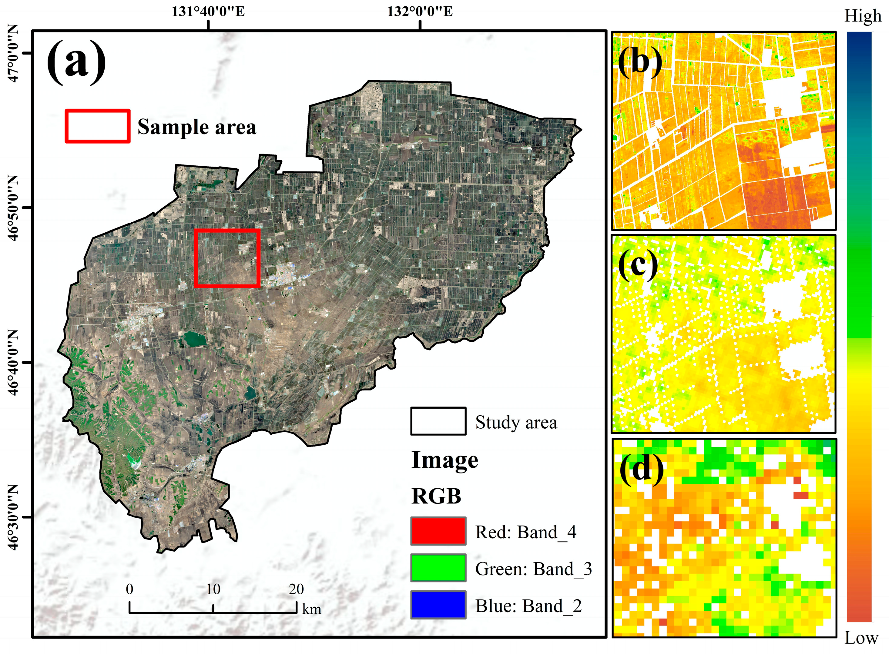
We compared the soil organic matter mapping results from this study with data from existing studies (Figure 7). The comparative data came from the China National Soil Information Product (spatial resolution of 90 m) developed by Liu et al. (2021) [42] and the Global Gridded Soil Information Product (spatial resolution of 250 m) developed by Hengl et al. [28,43]. A comparative analysis was conducted between the soil organic matter (SOM) distribution map generated in this study and existing datasets, specifically the 90 m resolution China Soil Information Product (CSIP) developed by Liu et al. and the 250 m resolution global gridded soil information product by Hengl et al. Sentinel-2 imagery from 2020 was utilized in our work. A representative sample area exhibiting a distinct dark-to-light color gradient was selected from true-color composites for detailed comparison. Our SOM map reveals a general decreasing trend from north to south, a spatial pattern consistent with the broad distributions observed in the two aforementioned reference products. In contrast, the other two datasets exhibit greater spatial heterogeneity and fail to capture this clear gradation in soil properties. The mapping methodology employed in this study demonstrates superior accuracy, enabling a more detailed representation of soil environmental characteristics. Consequently, our SOM predictions are more accurate and consistent at finer scales, exhibiting improved cartographic trends, spatial resolution, and overall precision. Therefore, the results presented herein provide a more comprehensive and detailed depiction of the spatial distribution of SOM within the study area.

5. Conclusions

This study systematically evaluated the spatiotemporal combination strategies and model optimization mechanisms for remote sensing-based mapping of cropland SOM under different climatic conditions, using multi-temporal Sentinel-2 imagery and environmental variables from 2019 to 2021. The results indicate that multi-temporal imagery generally outperforms single-date imagery, with combined use of bare soil and crop growth period images showing notable differences across climatic years: in drought years, bare soil information contributed most to model predictions; in normal years, the dual-date fusion achieved the best performance; while in flood years, bare soil imagery dominated the prediction accuracy. The incorporation of environmental variables significantly enhanced model performance, particularly under conditions of limited remote sensing information or strong ecological process influence, with temperature consistently identified as the most influential factor, highlighting the dominant role of water–heat conditions in controlling SOM spatial distribution. Furthermore, feature selection effectively reduced redundant information, improving model robustness and generalization, with the greatest impact observed in climatically stable years. From a methodological perspective, this study’s first innovation lies in explicitly linking interannual climatic variability to the optimization of remote sensing temporal combinations, establishing a climate-adaptive SOM mapping framework that avoids the inaccuracy of fixed-period strategies in extreme climates. The second innovation is the development of a RF-RFE feature selection method tailored to complex climatic scenarios, which adaptively retains key features to ensure model stability across different climatic conditions—an improvement over traditional feature selection methods that lack scenario adaptability. Overall, this study demonstrates the feasibility of integrating differentiated spatiotemporal combinations, environmental variables, and feature selection to enhance SOM mapping accuracy under complex climatic conditions, providing scientific support and technical guidance for regional cropland quality monitoring, agricultural resource management, and carbon cycle assessment.

References

1. Carter, M.R. Soil quality for sustainable land management: Organic matter and aggregation interactions that maintain soil functions. Agron. J. 2002, 94, 38–47. [Google Scholar] [CrossRef]
2. Rumpel, C.; Kögel-Knabner, I. Deep soil organic matter—A key but poorly understood component of terrestrial C cycle. Plant Soil 2011, 338, 143–158. [Google Scholar] [CrossRef]
3. Soussana, J.-F.; Tallec, T.; Blanfort, V. Mitigating the greenhouse gas balance of ruminant production systems through carbon sequestration in grasslands. Animal 2010, 4, 334–350. [Google Scholar] [CrossRef]
4. Lal, R. Global potential of soil carbon sequestration to mitigate the greenhouse effect. Crit. Rev. Plant Sci. 2003, 22, 151–184. [Google Scholar] [CrossRef]
5. Gerke, J. The central role of soil organic matter in soil fertility and carbon storage. Soil Syst. 2022, 6, 33. [Google Scholar] [CrossRef]
6. Boyle, M.; Frankenberger, W., Jr.; Stolzy, L. The influence of organic matter on soil aggregation and water infiltration. J. Prod. Agric. 1989, 2, 290–299. [Google Scholar] [CrossRef]
7. Liu, X.; Zhang, X.; Wang, Y.; Sui, Y.; Zhang, S.; Herbert, S.; Ding, G. Soil degradation: A problem threatening the sustainable development of agriculture in Northeast China. Plant Soil Environ. 2010, 56, 87–97. [Google Scholar] [CrossRef]
8. Gomiero, T. Soil degradation, land scarcity and food security: Reviewing a complex challenge. Sustainability 2016, 8, 281. [Google Scholar] [CrossRef]
9. Ma, Y.; Minasny, B.; Malone, B.P.; Mcbratney, A.B. Pedology and digital soil mapping (DSM). Eur. J. Soil Sci. 2019, 70, 216–235. [Google Scholar] [CrossRef]
10. Ma, Y.; Wu, H.; Wang, L.; Huang, B.; Ranjan, R.; Zomaya, A.; Jie, W. Remote sensing big data computing: Challenges and opportunities. Future Gener. Comput. Syst. 2015, 51, 47–60. [Google Scholar] [CrossRef]
11. Zhang, M.; Zhang, M.; Yang, H.; Jin, Y.; Zhang, X.; Liu, H. Mapping regional soil organic matter based on sentinel-2a and modis imagery using machine learning algorithms and google earth engine. Remote Sens. 2021, 13, 2934. [Google Scholar] [CrossRef]
12. Emadi, M.; Taghizadeh-Mehrjardi, R.; Cherati, A.; Danesh, M.; Mosavi, A.; Scholten, T. Predicting and mapping of soil organic carbon using machine learning algorithms in Northern Iran. Remote Sens. 2020, 12, 2234. [Google Scholar] [CrossRef]
13. Chen, D.; Chang, N.; Xiao, J.; Zhou, Q.; Wu, W. Mapping dynamics of soil organic matter in croplands with MODIS data and machine learning algorithms. Sci. Total Environ. 2019, 669, 844–855. [Google Scholar] [CrossRef]
14. Li, M.; Yan, Y. Comparative analysis of machine-learning models for soil moisture estimation using high-resolution remote-sensing data. Land 2024, 13, 1331. [Google Scholar] [CrossRef]
15. Dou, X.; Wang, X.; Liu, H.; Zhang, X.; Meng, L.; Pan, Y.; Yu, Z.; Cui, Y. Prediction of soil organic matter using multi-temporal satellite images in the Songnen Plain, China. Geoderma 2019, 356, 113896. [Google Scholar] [CrossRef]
16. Sommer, S.; Hill, J.; Megier, J. The potential of remote sensing for monitoring rural land use changes and their effects on soil conditions. Agric. Ecosyst. Environ. 1998, 67, 197–209. [Google Scholar] [CrossRef]
17. Chabrillat, S.; Ben-Dor, E.; Cierniewski, J.; Gomez, C.; Schmid, T.; van Wesemael, B. Imaging spectroscopy for soil mapping and monitoring. Surv. Geophys. 2019, 40, 361–399. [Google Scholar] [CrossRef]
18. Murphy, B. Impact of soil organic matter on soil properties—A review with emphasis on Australian soils. Soil Res. 2015, 53, 605–635. [Google Scholar] [CrossRef]
19. Zhang, Y.; Luo, C.; Zhang, Y.; Gao, L.; Wang, Y.; Wu, Z.; Zhang, W.; Liu, H. Integration of bare soil and crop growth remote sensing data to improve the accuracy of soil organic matter mapping in black soil areas. Soil Tillage Res. 2024, 244, 106269. [Google Scholar] [CrossRef]
20. Zhu, X.; Cai, F.; Tian, J.; Williams, T.K.-A. Spatiotemporal fusion of multisource remote sensing data: Literature survey, taxonomy, principles, applications, and future directions. Remote Sens. 2018, 10, 527. [Google Scholar] [CrossRef]
21. Xue, J.; Su, B. Significant remote sensing vegetation indices: A review of developments and applications. J. Sens. 2017, 2017, 1353691. [Google Scholar] [CrossRef]
22. Yang, J.; Gong, P.; Fu, R.; Zhang, M.; Chen, J.; Liang, S.; Xu, B.; Shi, J.; Dickinson, R. The role of satellite remote sensing in climate change studies. Nat. Clim. Chang. 2013, 3, 875–883. [Google Scholar] [CrossRef]
23. Ben-Dor, E.; Irons, J.; Epema, G. Soil reflectance. Remote Sens. Earth Sci. Man. Remote Sens. 1999, 3, 111–188. [Google Scholar]
24. Weil, R.R.; Magdoff, F. Significance of soil organic matter to soil quality and health. In Soil Organic Matter in Sustainable Agriculture; CRC Press: Boca Raton, FL, USA, 2004; pp. 1–43. [Google Scholar]
25. Panigada, C.; Tagliabue, G.; Zaady, E.; Rozenstein, O.; Garzonio, R.; Di Mauro, B.; De Amicis, M.; Colombo, R.; Cogliati, S.; Miglietta, F.; et al. A new approach for biocrust and vegetation monitoring in drylands using multi-temporal Sentinel-2 images. Prog. Phys. Geogr. Earth Environ. 2019, 43, 496–520. [Google Scholar] [CrossRef]
26. Babaeian, E.; Sadeghi, M.; Jones, S.B.; Montzka, C.; Vereecken, H.; Tuller, M. Ground, proximal, and satellite remote sensing of soil moisture. Rev. Geophys. 2019, 57, 530–616. [Google Scholar] [CrossRef]
27. Zhang, Y.; Luo, C.; Zhang, W.; Wu, Z.; Zang, D. Mapping Soil Organic Matter in Black Soil Cropland Areas Using Remote Sensing and Environmental Covariates. Agriculture 2025, 15, 339. [Google Scholar] [CrossRef]
28. Kong, D.; Luo, C.; Liu, H. Integrative remote sensing and machine learning approaches for SOC and TN spatial distribution: Unveiling C: N ratio in Black Soil region. Soil Tillage Res. 2026, 255, 106809. [Google Scholar] [CrossRef]
29. Jin, X.; Du, J.; Liu, H.; Wang, Z.; Song, K. Remote estimation of soil organic matter content in the Sanjiang Plain, Northest China: The optimal band algorithm versus the GRA-ANN model. Agric. For. Meteorol. 2016, 218–219, 250–260. [Google Scholar] [CrossRef]
30. Guyon, I.; Weston, J.; Barnhill, S.; Vapnik, V. Gene selection for cancer classification using support vector machines. Mach. Learn. 2002, 46, 389–422. [Google Scholar] [CrossRef]
31. Svetnik, V.; Liaw, A.; Tong, C.; Culberson, J.C.; Sheridan, R.P.; Feuston, B.P. Random forest: A classification and regression tool for compound classification and QSAR modeling. J. Chem. Inf. Comput. Sci. 2003, 43, 1947–1958. [Google Scholar] [CrossRef]
32. Liu, S.; An, N.; Yang, J.; Dong, S.; Wang, C.; Yin, Y. Prediction of soil organic matter variability associated with different land use types in mountainous landscape in southwestern Yunnan province, China. Catena 2015, 133, 137–144. [Google Scholar] [CrossRef]
33. Zhang, D.; Zhou, G. Estimation of soil moisture from optical and thermal remote sensing: A review. Sensors 2016, 16, 1308. [Google Scholar] [CrossRef] [PubMed]
34. Samuel-Rosa, A.; Heuvelink, G.; Vasques, G.; Anjos, L. Do more detailed environmental covariates deliver more accurate soil maps? Geoderma 2015, 243–244, 214–227. [Google Scholar] [CrossRef]
35. Xiao, X.; He, Q.; Ma, S.; Liu, J.; Sun, W.; Lin, Y.; Yi, R. Environmental variables improve the accuracy of remote sensing estimation of soil organic carbon content. Sci. Rep. 2024, 14, 18964. [Google Scholar] [CrossRef]
36. Chen, Y.; Ma, L.; Yu, D.; Zhang, H.; Feng, K.; Wang, X.; Song, J. Comparison of feature selection methods for mapping soil organic matter in subtropical restored forests. Ecol. Indic. 2022, 135, 108545. [Google Scholar] [CrossRef]
37. Guo, L.; Fu, P.; Shi, T.; Chen, Y.; Zeng, C.; Zhang, H.; Wang, S. Exploring influence factors in mapping soil organic carbon on low-relief agricultural lands using time series of remote sensing data. Soil Tillage Res. 2021, 210, 104982. [Google Scholar] [CrossRef]
38. Abdulraheem, M.I.; Zhang, W.; Li, S.; Moshayedi, A.J.; Farooque, A.A.; Hu, J. Advancement of remote sensing for soil measurements and applications: A comprehensive review. Sustainability 2023, 15, 15444. [Google Scholar] [CrossRef]
39. Samadzadegan, F.; Toosi, A.; Dadrass Javan, F. A critical review on multi-sensor and multi-platform remote sensing data fusion approaches: Current status and prospects. Int. J. Remote Sens. 2025, 46, 1327–1402. [Google Scholar] [CrossRef]
40. Chen, M.; Qian, Z.; Boers, N.; Jakeman, A.J.; Kettner, A.J.; Brandt, M.; Kwan, M.-P.; Batty, M.; Li, W.; Zhu, R.; et al. Iterative integration of deep learning in hybrid Earth surface system modelling. Nat. Rev. Earth Environ. 2023, 4, 568–581. [Google Scholar] [CrossRef]
41. Di, X.; Wang, X. Method for Zoning Corn Based on the NDVI and the Improved SOM-K-Means Algorithm. J. ASABE 2023, 66, 943–953. [Google Scholar] [CrossRef]
42. Liu, F.; Wu, H.; Zhao, Y.; Li, D.; Yang, J.-L.; Song, X.; Shi, Z.; Zhu, A.-X.; Zhang, G.-L. Mapping high resolution national soil information grids of China. Sci. Bull. 2021, 67, 328–340. [Google Scholar] [CrossRef] [PubMed]
43. Hengl, T.; Mendes de Jesus, J.; Heuvelink, G.B.M.; Ruiperez Gonzalez, M.; Kilibarda, M.; Blagotić, A.; Shangguan, W.; Wright, M.N.; Geng, X.; Bauer-Marschallinger, B.; et al. SoilGrids250m: Global gridded soil information based on machine learning. PLoS ONE 2017, 12, e0169748. [Google Scholar] [CrossRef] [PubMed]
Figure 1. Basic flowchart of the study.
Agronomy 15 02714 g001
Figure 2. Overview of the study area.
Agronomy 15 02714 g002
Figure 3. Annual precipitation in the study area.
Agronomy 15 02714 g003
Figure 4. (ac) represent the predicted spatial distributions of SOM for 2019, 2020, and 2021, respectively.
Agronomy 15 02714 g004
Figure 5. Comparison of R2 and RMSE between single-period and dual-period imagery across different years.
Agronomy 15 02714 g005
Figure 6. (ac) represent the importance ranking of environmental variables in 2019, 2020, and 2021, respectively.
Agronomy 15 02714 g006
Figure 7. Comparison of mapping results between this study and other studies. (a) Sentinel-2 image of the study area from May 2020; (b) Zoomed-in view of the SOM map from this study; (c) Zoomed-in view of the corresponding map from Liu et al. (2021) [42]; (d) Zoomed-in view of the corresponding map from Hengl et al. (2017) [43].
Agronomy 15 02714 g007