Article

A New Approach to Sensible Heat Flux via CFD-Surface Renewal Integration

School of Agricultural Engineering, Jiangsu University, Zhenjiang 212013, China
*
Author to whom correspondence should be addressed.
Agronomy 2025, 15(12), 2708; https://doi.org/10.3390/agronomy15122708
Submission received: 8 October 2025 / Revised: 19 November 2025 / Accepted: 21 November 2025 / Published: 25 November 2025

Abstract

This study integrates surface renewal theory (SR) with computational fluid dynamics (CFD) models to explore the estimation of sensible heat flux in tea plantations. SR describes the turbulent transport processes at the air–water interface and has been widely applied in sensible heat flux estimation. However, its practical application faces challenges, such as determining the calibration coefficient (α) and the reliability of high-frequency temperature sensors (10 hz). This research addresses these issues by combining large eddy simulation (LES) models with CFD simulations to simulate high-frequency temperature variations in flat tea plantation fields. The results indicate that the LES model accurately simulates temperature fluctuations across different timescales (1 min, 30 min), with R2 values ranging from 0.72 to 0.99, suggesting its suitability for precise sensible heat flux calculations. Furthermore, a new method for determining the calibration coefficient α using CFD simulations is proposed, which accounts for variations in atmospheric stability and terrain, thus improving the accuracy and applicability of SR in heterogeneous environments. The findings demonstrate that the CFD-based approach offers a cost-effective alternative to traditional eddy covariance systems, simplifying field measurements and enhancing the precision of sensible heat flux calculations under various atmospheric conditions (sunny, cloudy, overcast, nighttime), thereby broadening the potential applications of surface renewal theory in crop water requirement research.

1. Introduction

Combining high-frequency temperature observation data with the surface renewal theory enables highly accurate estimation of the evapotranspiration of target vegetation [1,2,3,4]. Evapotranspiration accounts for 80–95% of total farmland water consumption, serving as a core link in the agricultural water cycle. Accurate ET estimation can address the blindness of irrigation management and realize the early warning of crop water stress, which is crucial for optimizing water use efficiency and ensuring agricultural sustainability. Although SR theory has been widely applied in fields such as crop water requirement estimation [5,6,7,8], in practical applications, some key issues remain inadequately resolved [9,10].
With the development of CFD technology, researchers have begun to recognize the potential of CFD in the field of meteorology. Li et al. [11] studied the sensitivity of the wind field using LES, and pointed out that, as the grid resolution increases, the CFD model can better capture the spatiotemporal distribution of small-scale turbulence. Sun et al. [12] conducted a numerical analysis of meso-scale and large-scale flow fields using the LES model, and found that the large-scale flow fields can better reflect the vertical fluctuations of the near-surface wind fields. Although existing CFD studies mainly focus on the changes in wind speed and direction [13,14,15,16], they provide theoretical and methodological support for using CFD to solve the problem of estimating vegetation evapotranspiration by combining high-frequency temperature with the surface renewal method. It is also expected to provide new ideas and methods for solving existing problems.
The determination of the calibration coefficient α (full name: calibration coefficient for heat exchange efficiency of near-surface air parcels) is a crucial and complex issue when using the surface renewal method to estimate sensible heat flux. It is introduced by scaling the local average gradient of air temperature with the temperature step change in the air microparcel updated per unit ground area, and is primarily used to describe the uniformity of heating in the air [15]. An air microparcel refers to a small-volume air unit with relatively uniform physical properties and dynamic motion in the near-surface atmosphere (0.1–2 m above the ground, i.e., the crop canopy area), which is distinct from the “air mass” in meteorology in terms of scale and research scenarios. Typically, α is set to 1 to indicate uniform heating (the temperature of a single measurement point can represent the average temperature of the entire region). However, its value is influenced by various factors, such as crop type and meteorological conditions, necessitating calibration using independent flux observation instruments, such as eddy covariance systems. Due to the high cost and operational complexity of eddy covariance systems, the widespread application of the surface renewal method is limited. To address this, Castellvi et al. [17] combined this method with the Monin–Obukhov similarity theory—a core theory in atmospheric boundary layer meteorology that uses the Monin–Obukhov length (L) to characterize the balance between buoyancy and turbulent viscous forces—and derived an analytical solution for the calibration coefficient under specific meteorological conditions. However, the accuracy of this method remains questionable in complex terrains, such as mountainous areas and densely built environments.
Additionally, fine-wire thermocouples have a shorter temperature response time but are more prone to breakage and have a shorter lifespan, particularly small-diameter thermocouples (e.g., 13 μm and 25 μm Type E) [18]. In the estimation of sensible heat flux above the canopy in tea plantations, Hu et al. [19] found that high-frequency temperature sensors often produce anomalous values (“dead points”) in high-temperature (≥35 °C), high-humidity (≥85%) or low-temperature (≤5 °C), high-humidity environments. Moreover, these sensors are prone to corrosion and damage in harsh environments, which can affect the reliability, continuity, and accuracy of the data.
Large eddy simulation (LES) is a numerical method for simulating turbulent flow that directly simulates large-scale eddies (dominant in momentum and energy transfer) and parameterizes small-scale eddies using subgrid-scale models (e.g., Smagorinsky model), balancing computational accuracy and efficiency. Compared with traditional CFD methods (e.g., RANS models), LES avoids high-frequency information loss caused by “averaging processing”, making it suitable for simulating small-scale turbulent motion that drives high-frequency temperature variations. However, LES also has limitations such as high computational cost and slow speed.
To address this issue, the present study aims to construct a CFD model of the plant canopy and near-surface atmosphere, using the LES turbulence model to quantitatively analyze the thermal environment characteristics and vorticity distribution near the canopy in open areas (flat regions without tall buildings within 50 m, no dense trees with DBH < 10 cm and spacing ≥ 10 m, and slope < 5°) [20,21,22,23]. Temperature monitoring points will be designed to focus on the temperature variation trends at specific canopy heights and the dynamic changes in calibration coefficients, with the CFD model’s predictions being validated against experimental data to provide theoretical and data support.
This study aims to verify the feasibility of using the CFD model to calculate high-frequency temperatures and calibration coefficients, offering support for the estimation of sensible heat flux using surface renewal theory in canopy environments [24,25,26,27]. Additionally, it will provide a deeper analysis of the applicability and underlying mechanisms of surface renewal theory under varying environmental conditions.

2. Materials and Methods

2.1. Test Tea Garden Experiments

The experiment was conducted at the Dantu Tea Plantation in Jiangsu Province (32°01′35″ N, 119°40′21″ E) as shown in Figure 1. The tea plantation is situated in the gently sloping hills of the middle and lower reaches of the Yangtze River in China, with an average altitude of 18.5 m. This area experiences a subtropical climate, with an average annual precipitation of approximately 1029 mm and an average temperature of about 288.6 K. As one of the primary production regions for China’s premium green tea, the experimental site features 7-year-old Mao Lu (Maolu) tea plants. The soil type of the experimental site is yellow-brown soil, with a loose texture and good water retention capacity. The agricultural management measures include regular pruning (twice a year), organic fertilizer application (once in spring), and drip irrigation (when soil moisture content is below 60% of field capacity). During the observation period (April–October 2023), the tea plants went through sprouting, growing, and dormancy stages, with the main observation period focusing on the summer growing stage (late July to mid-August).

2.2. Experimental Design and Data Analysis Methods

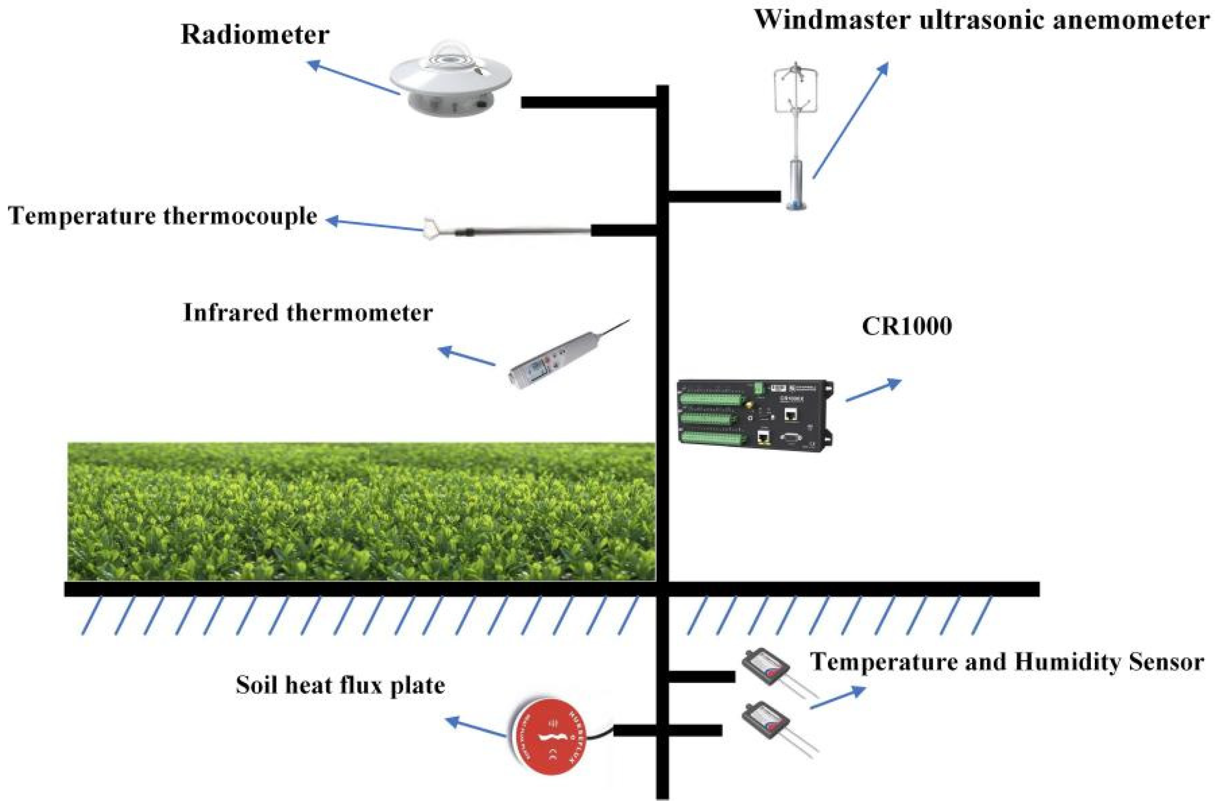
In this experiment, the micrometeorological observation system for surface renewal in the tea plantation primarily consisted of a data logger (CR3000, Campbell Scientific, Logan, UT, USA), a temperature and humidity sensor (HC2S3, Campbell Scientific, USA), a four-component net radiometer (CNR4, Kipp & Zonen, Delft, The Netherlands), a three-dimensional ultrasonic anemometer (Windmaster, Gill, UK), a soil heat flux plate (HFP01SC, Hukseflux, Delft, The Netherlands), an air temperature and humidity sensor (HC2S3, Campbell Scientific, Logan, UT, USA), Type E thermocouples (COCO-03, Omega, Norwalk, CT, USA), and an infrared temperature sensor (SI-111, Apogee Instruments, Logan, UT, USA), as shown in Figure 2.
To evaluate the accuracy of the model’s computational results in fitting the experimental data and assess the precision of the surface renewal method in calculating sensible heat flux, the selected statistical variables and key analytical parameters include the correlation coefficients (R2, Pearson’s r), and three fundamental variables in the sensible heat flux equation: Ta, representing the amplitude or magnitude of high-frequency temperature slope variations (K); τ , denoting the period of slope changes (s); and T a / τ , indicating the slope value of these variations. A high correlation in R2, Pearson’s r indicates a strong relationship between the simulated and observed values, reflecting a high degree of agreement between the model predictions and the experimental data. The calculation Equations (4) and (5) are as follows [28]:
R 2 = 1 i = 1 n ( y i y ^ i ) 2 i = 1 n ( y i y ¯ ) 2
p e a r s o n s = ( x x ¯ ) ( y y ¯ ) ( x x ¯ ) 2 × ( y y ¯ ) 2
In the equation, y i represents the actual observed values (K); y ^ i represents the model-predicted values (K); y ¯ represents the mean of the observed values (K); and x ¯ represents the mean of the simulated values (K).

2.3. Estimation of Sensible Heat Flux by the SR Method

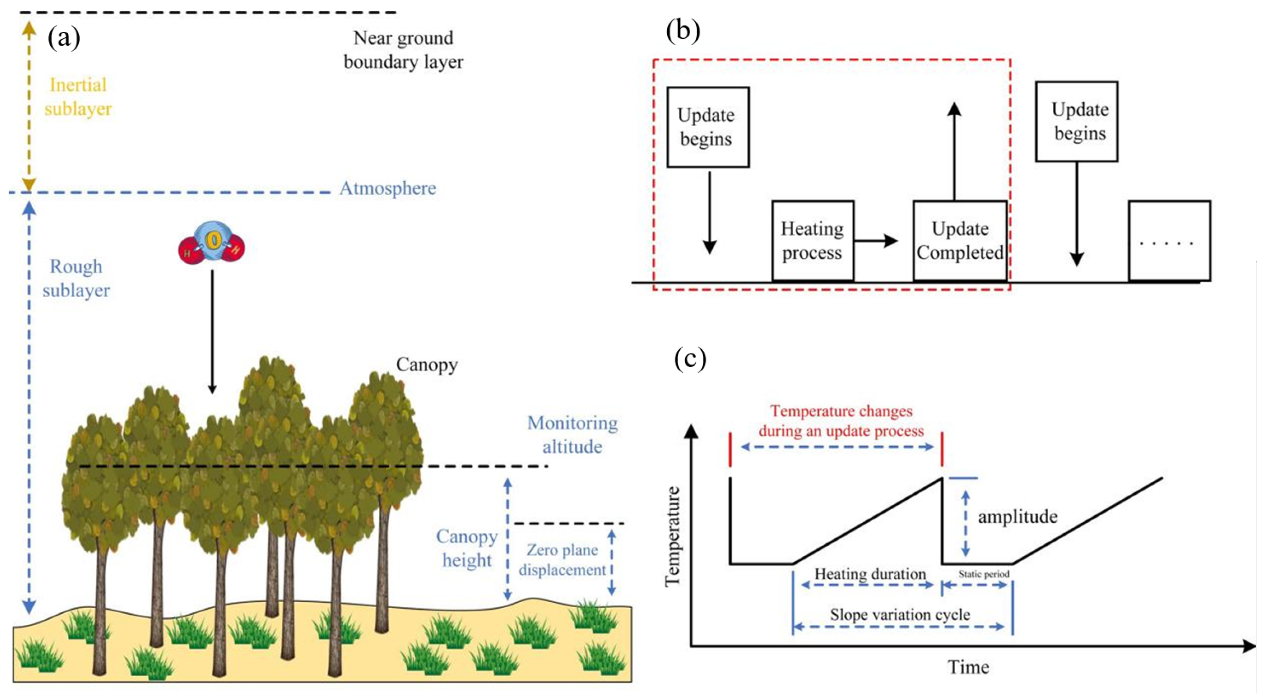
The fundamental concept of sensible heat flux is that the net heat exchange is determined by all slope events (temperature rise/fall processes showing slope-like changes) occurring over a specified time period, as depicted by the slope changes in Figure 3.
From this, the mathematical expression for sensible heat flux (Hsr) can be derived [29,30]. Equations (3) and (4) are as follows:
H sr = ρ C p T a L r + L q ( α z ) = ρ C p T a τ ( α z )
α = { [ z d k π φ h ( ζ ) τ u * ] 1 / 2 [ z 2 k π z * φ h ( ζ ) τ u * ] 1 / 2 if   ( z d ) > z * if   h ( z d ) z *
In the equation, ρ and C p represent air density (kg·m−3) and specific heat at a constant pressure of air (J·kg−1·K−1), respectively; a represents the amplitude or amplitude of high-frequency temperature ramp change (K); and α describes the uniformity of heating in a unit volume of air. When the air is heated evenly, α reaches 1; z represents the observation height of the high-frequency temperature sensor (m); h represents the canopy height (m); d is the zero plane displacement height (m); ζ is the stability parameter or a dimensionless buoyancy parameter defined as ζ = ( z d ) / L o , and Lo is the Obukhov length [31,32,33,34]; τ denotes the ramp change period (s), which is the sum of the time period for the temperature to change in a ramp-like manner (or heating duration, Lr) and the stationary period (Lq) during which the temperature does not change with time (s). Both Ta and τ can be solved using the temperature structure function Sn(r) proposed by Liu et al. [24].

2.4. CFD Method for Flow Field Simulation

2.4.1. Model Construction and Mesh Generation

In this study, the temperature and humidity fields of both the flat and sloped tea plantations in Dantu were simulated. The tea plantations are located in the gently sloping hilly areas of the middle and lower reaches of the Yangtze River in China, with an average elevation of 18.5 m. The fluid flow in the model adheres to four fundamental conservation laws: mass conservation, momentum conservation, energy conservation, and species conservation. A three-dimensional model with a 1:1 scale was constructed based on the actual dimensions of the tea plantations. The simplification made is that the ground surface evaporation was neglected, and the focus was solely on the canopy evaporation. The plant canopy model adopts a one-layer canopy energy balance model, and key parameters such as inertial drag coefficient (0.25) and viscous drag coefficient (0.01) are defined to characterize the resistance of tea plants to airflow. The construction of the geometric model and the mesh generation of the tea plantations are shown in Supplementary Figure S1.
Structured meshing was performed using the Workbench Icem module, with mesh refinement applied to the canopy region and the rough sublayer above the canopy. Mesh quality was controlled according to the EquiAngle Skewness criterion, ensuring that the mesh met the necessary standards for subsequent simulations.

2.4.2. Boundary Condition Setup

The eastern boundary of the external flow domain was specified as a velocity inlet, while the southern, western, and northern boundaries were defined as pressure outlets. The ground surface was assigned a wall boundary condition with convective heat transfer, and the plant canopy was modeled as a coupled heat transfer wall. The material properties are provided in Table 1.

2.4.3. Control Equations and Numerical Formats

The solver selected for this study was ANSYS FLUENT 2022R1, utilizing a transient simulation approach. A second-order upwind scheme was employed for spatial discretization. The turbulence models selected were the LES model. To simulate the impact of solar radiation on the tea plantation environment, the discrete ordinates (DO) radiation model and the solar ray tracing model were applied. The Boussinesq model was adopted to account for the thermal buoyancy effects of air and water vapor. The operating temperature was set to the ambient environmental temperature. The couple algorithm was employed for pressure–velocity coupling.
The CFD model adheres to the fundamental governing equations during the solution process, including the continuity equation, momentum equation, energy equation, and species transport equation. The equations are as follows [35].
Continuity equation:
ρ t + div ( ρ u i ) = 0
Momentum equation:
( ρ u ) t + div ( ρ u v ) = P x + div ( μ grad u ) + S u
( ρ v ) t + div ( ρ υ v ) = P y + div ( μ grad υ ) + S υ
( ρ ω ) t + div ( ρ ω v ) = P z + div ( μ grad ω ) + S ω
Energy equation:
( ρ ω ) t + div ( ρ ω v ) = P z + div ( μ grad ω ) + S ω
In the equation, t is time (s); υ is the velocity vector (m·s−1); u, v, w are the components of velocity in x, y, z directions (m·s−1); μ is the air turbulence viscosity (kg·m−1·s−1); T is the air temperature (K); k is the thermal conductivity of air (W·m−1·K−1); and ST is the energy source term (W).
The LES model separates instantaneous turbulent motion into large- and small-scale eddies via a filtering function. After filtering the continuity and momentum equations, the following equations are derived [36,37,38,39]:
ρ t + ρ u ˜ i x i = 0
ρ u ˜ i x i + ρ u ˜ i u ˜ j x j = p ˜ x j + x j ( μ i x i τ i j )
τ i j = 2 μ S ¯ i j + 1 3 τ k k δ i j
In the equation, ρ is the density of the mixed phase (kg·m−3); u ˜ i and u ˜ j are the velocity components in the i and j directions after filtering, respectively (m·s−1); p ˜ represents the filtered pressure (Pa); μ denotes the dynamic viscosity coefficient of the mixed phase (Ns·m−2); τ i j refers to the subgrid stress term (N·m−2); S ¯ i j indicates the average strain rate tensor (1/s); δ i j represents the Kronecker delta function; and τ k k stands for the isotropic part of the subgrid-scale stress (N·m−2).

2.4.4. Verification of Grid Independence

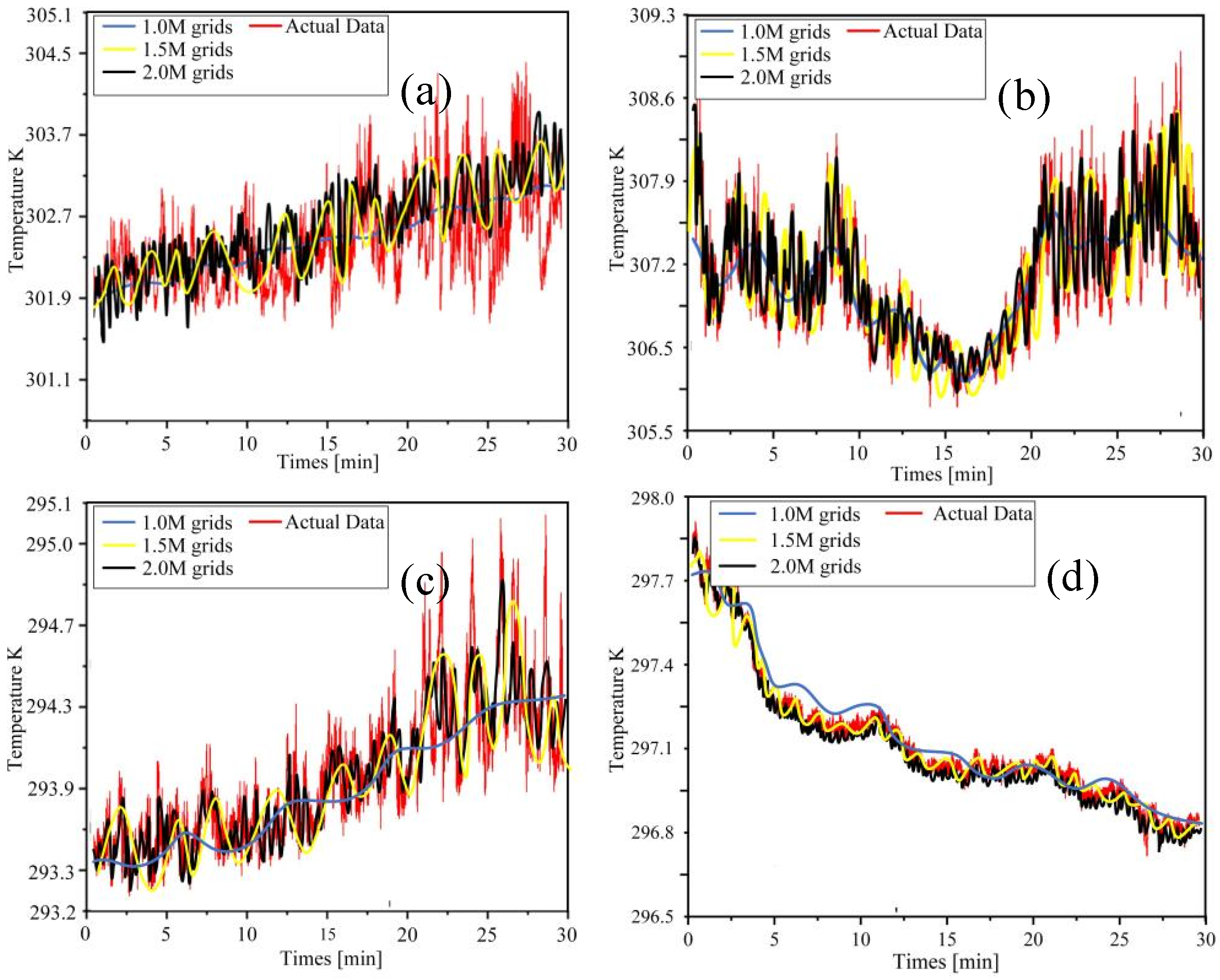
Based on large eddy simulation, a study on temperature changes under different weather conditions (sunny, cloudy, overcast, and nighttime) with different grid numbers was carried out, as shown in Figure 4. From the results, it can be seen that, as the number of grids increases from 1 million to 2 million, the simulated temperature fluctuation becomes closer to the actual temperature fluctuation data. This indicates that the greater the number of grids, the more accurately the transient temperature fluctuation characteristics can be identified. The simulated temperature fluctuation can better provide a more precise temperature dynamic basis for calculating the sensible heat flux using the surface renewal method, and can significantly improve the calculation accuracy of the sensible heat flux. In the following, the number of simulation grids is selected as 2.5 million to carry out relevant simulation research.

3. Results

3.1. Extraction and Application of the Flow Field Heat Flux Calibration Coefficient α Based on Large Eddy Simulation

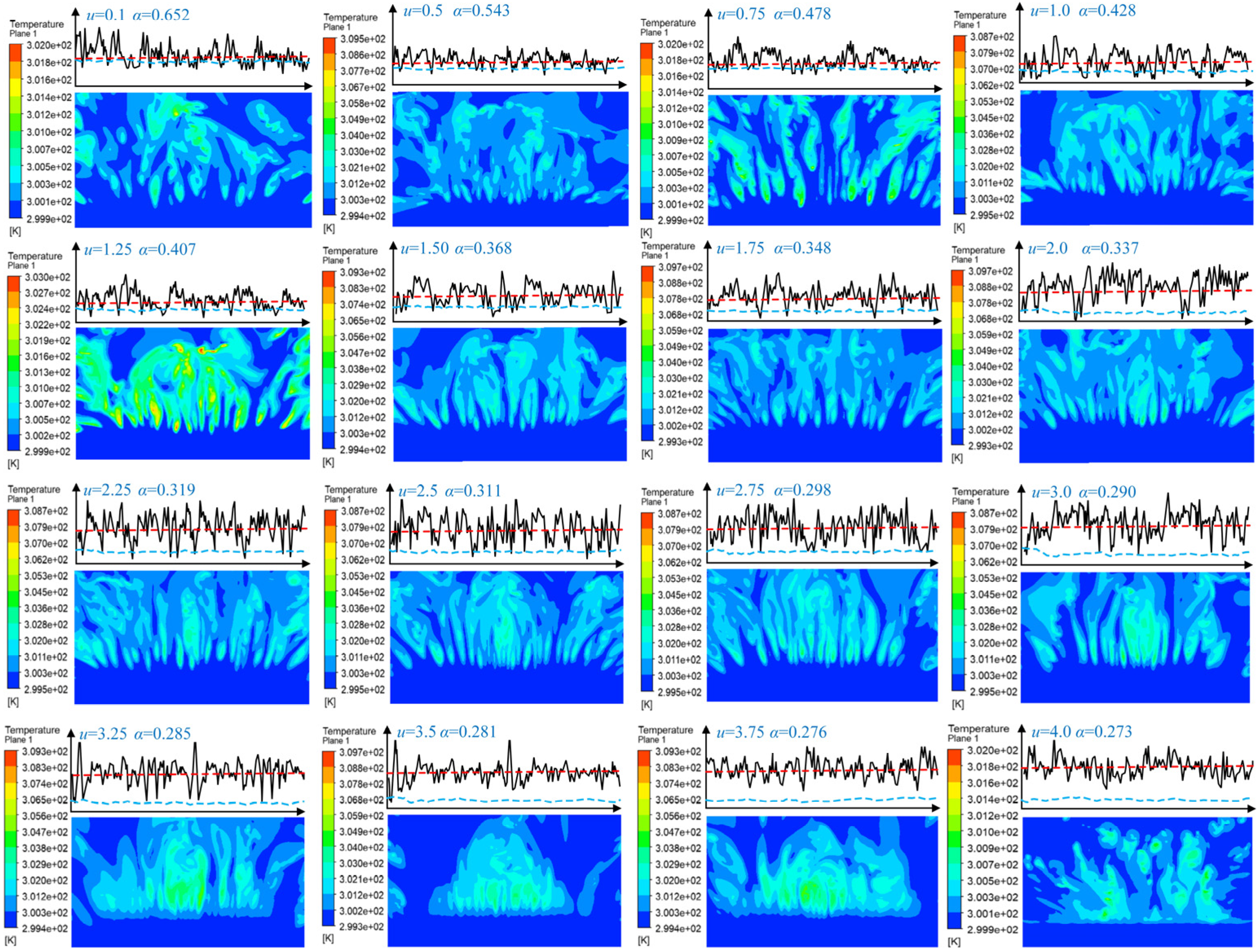
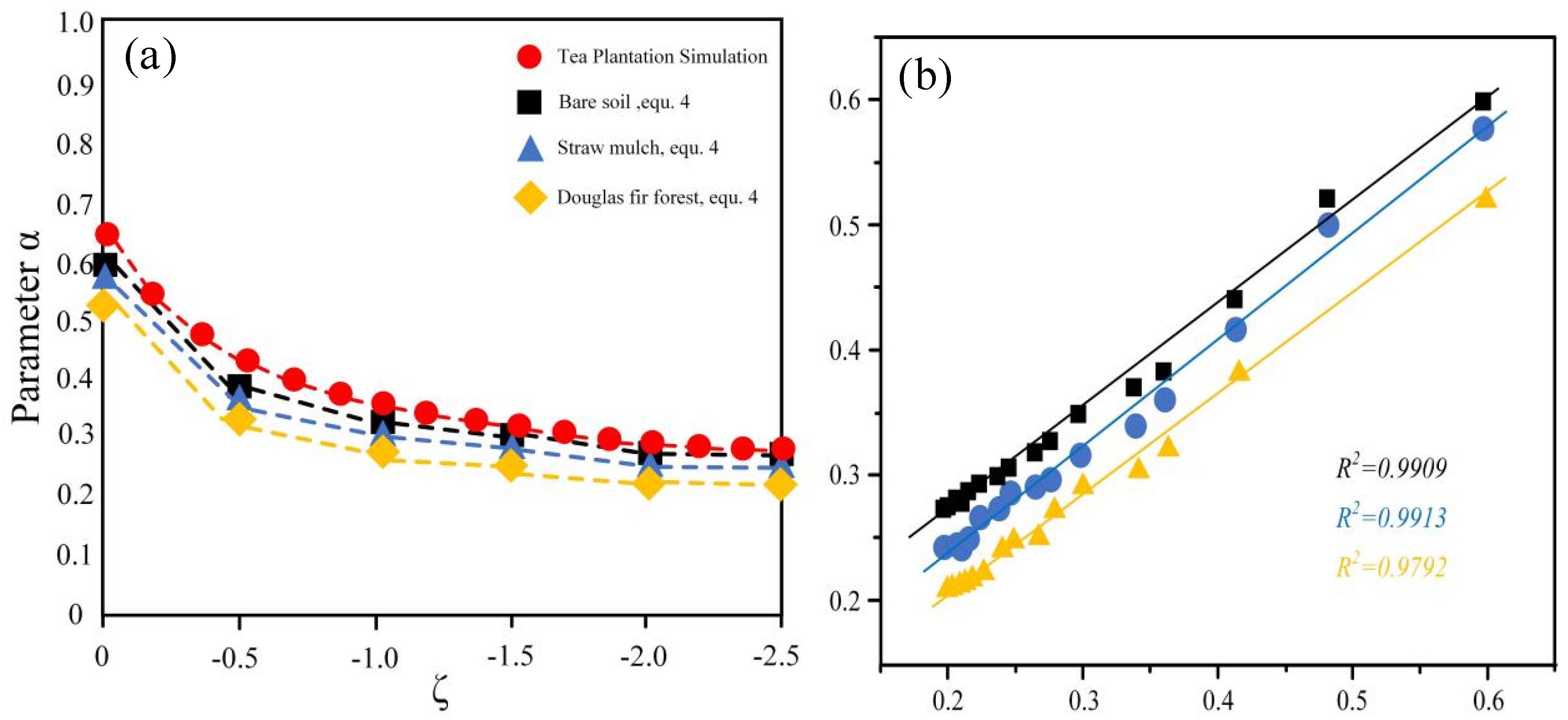
In order to investigate the variation in the flux calibration coefficient under different atmospheric stability parameters, this study constructed a three-dimensional model of a flat tea plantation and carried out CFD simulations, as shown in Figure 5. The three-dimensional model of the flat tea plantation covers the variation range of atmospheric stability parameters from 0 to −2.5. Each model underwent 16 simulations, with each simulation representing a specific atmospheric stability condition. By utilizing the simulation data, this study analyzed the average high-frequency temperature oscillations at the canopy height of 2 m and multiplied them by the calibration coefficient α. Subsequently, the obtained results were converted into the average temperature within the entire computational domain. In this way, the flux variations within the entire computational domain can be represented by the data from a single monitoring point.
It can be analyzed from Figure 6 that the calculated calibration coefficients exhibit a strong linear relationship with the coefficients proposed by Castellvi et al. [17]. Although there are some differences in the calibration coefficients among different plants, the deviations of these differences are relatively small, with the maximum error being approximately 0.1. This is because there are differences in canopy roughness among different crops, which lead to variations in the transition of near-surface airflow states. Nevertheless, the variation trends of the calibration coefficients remain consistent, with correlation coefficients of 0.9909, 0.9913, and 0.9792, respectively. This indicates that the changes in the calibration coefficients of different plants follow similar patterns.

3.2. Study on the Mechanism of the Surface Renewal Theory Based on Large Eddy Simulation

Based on Supplementary Figure S2, it can be concluded that the LES model produces more detailed results for temperature, water vapor, and vorticity. The LES model enables the observation of spatial temperature fluctuations and the temporal evolution of water vapor disturbances. The analysis reveals that the temperature fluctuations and water vapor disturbances follow an almost identical pattern, consistent with the theory proposed by Kermani and Shen [40]. Their theory posits that temperature fluctuations are driven by the continuous replenishment of liquid or air masses from below, which sustains the turbulent exchange at the interface (Supplementary Figure S3). This suggests that the fundamental cause of high-frequency temperature fluctuations, as described by the surface renewal theory, is the continuous variation in water vapor concentration within the space. At the same time, it also lays a theoretical and practical foundation for combining computational fluid dynamics with the surface renewal theory to calculate the sensible heat flux.

3.3. Analysis of High-Frequency Temperature Results from Actual and Simulated Data at Large Time Scales Under the Large Eddy Simulation

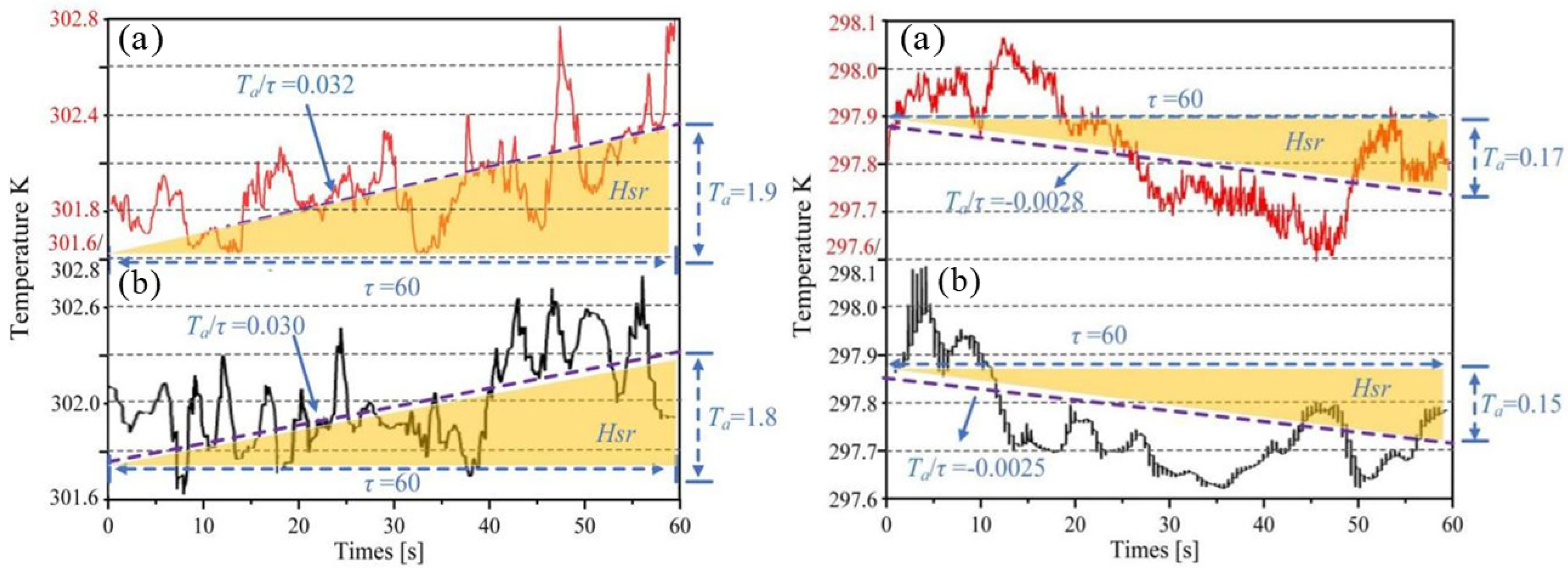
The high-frequency temperature data on a small time scale (60 s) for both daytime and nighttime (Figure 7) periods were analyzed in terms of temperature correlation (Supplementary Figure S4). The analysis revealed that both time periods exhibit a strong linear correlation.
The R2 during the daytime was 0.72 and the Pearson’s r was 0.82. The R2 at night was 0.85 and the Pearson’s r was 0.91. This indicates that the variation trends of the high-frequency temperature obtained through actuality and simulation over time were the same during both the daytime and the nighttime.
The coefficients for calculating sensible heat flux from high-frequency temperature actualities and simulations during the daytime were as follows: Ta values of 1.9 and 1.8, τ values of 60 for both, and T a / τ values of 0.032 and 0.030, respectively. For the nighttime, the actual and simulated coefficients were as follows: Ta values of 0.17 and 0.15, τ values of 60 for both, and T a / τ values of −0.0028 and −0.0025, respectively.
Therefore, it can be concluded that the high-frequency temperature variations and sensible heat flux values derived from actualities and simulations show a tendency towards consistency under both daytime and nighttime conditions on small time scales (60 s).

3.4. Analysis of High-Frequency Temperature Results from Actual and Simulated Data at Small and Large Time Scales Under the Large Eddy Simulation

Correlation analyses of actual and simulated high-frequency temperature values were performed across various conditions, including sunny day, cloudy day, overcast day, nighttime, and throughout the entire day. These analyses were conducted at larger time scales (30 min and 24 h).
It was observed that, at larger time scales, the simulated high-frequency temperature values for sunny day, cloudy day, overcast day, nighttime, and the entire day demonstrated a strong linear relationship with the actual values.
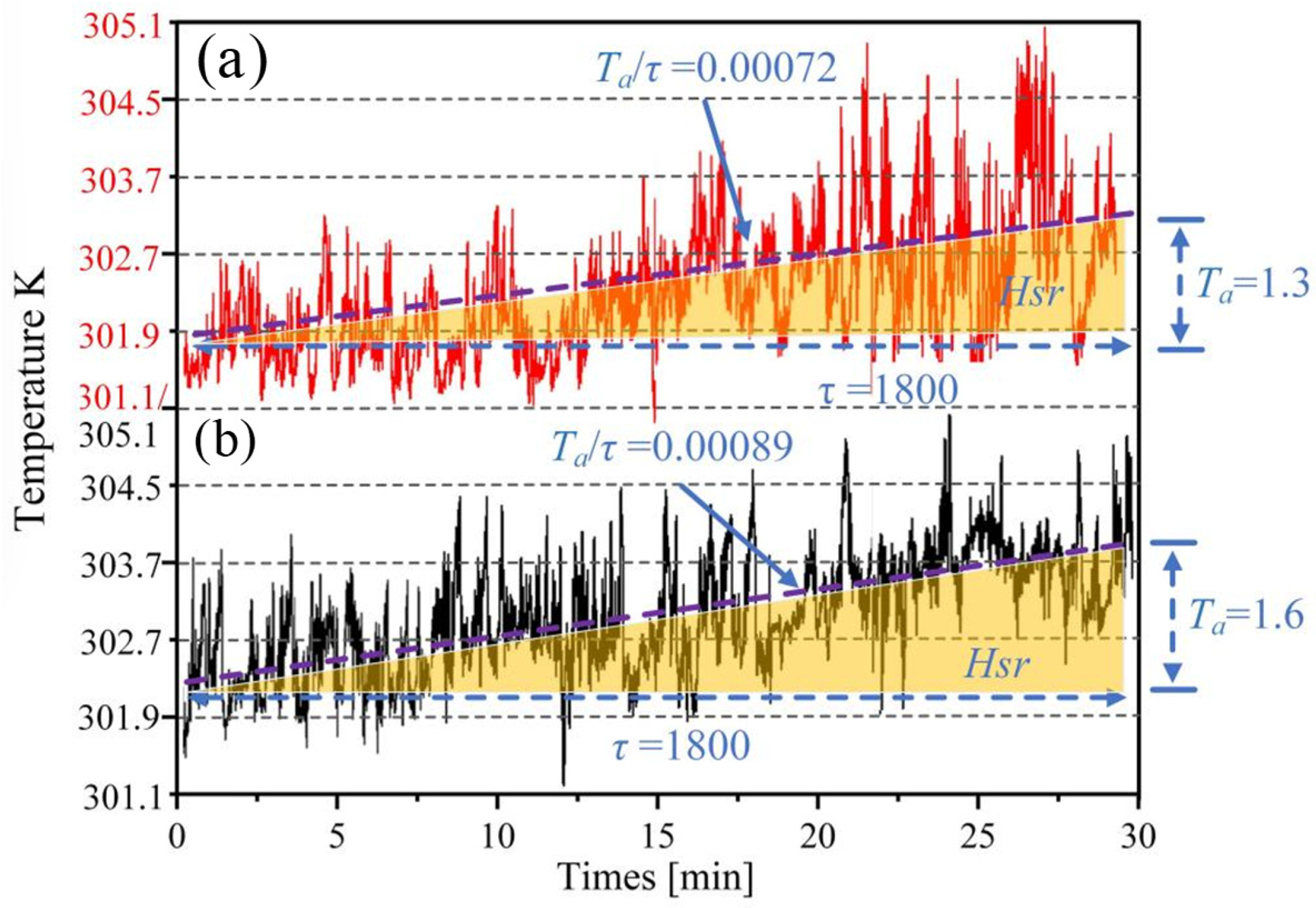
The boundary conditions for the tea garden on sunny days at larger time scales were established based on the foregoing content, with the time interval extended from the previous 60 s to 30 min. High-frequency temperature variations over this 30 min period for the LES model during the daytime were calculated using CFD simulations, as illustrated in Figure 8b. From the figure, it can be observed that the oscillation range of the simulated high-frequency temperature lies between 301.1 K and 305.1 K. As time progresses and radiation values increase, the temperature exhibits a gradual upward trend. Notably, the oscillation range and variation trend closely resemble the oscillation patterns of the actual daytime high-frequency temperatures presented in Figure 8a.
As illustrated in Figure 8, the coefficients for calculating sensible heat flux from actual and simulated high-frequency temperatures on clear days at larger time scales are as follows: Ta values of 1.3 and 1.6, τ values of 1800 for both, and T a / τ values of 0.00072 and 0.00089, respectively.
Thus, it can be concluded that the high-frequency temperature variations and calculated sensible heat flux values obtained from both actualities and simulations exhibit consistency at larger time scales on a sunny day.
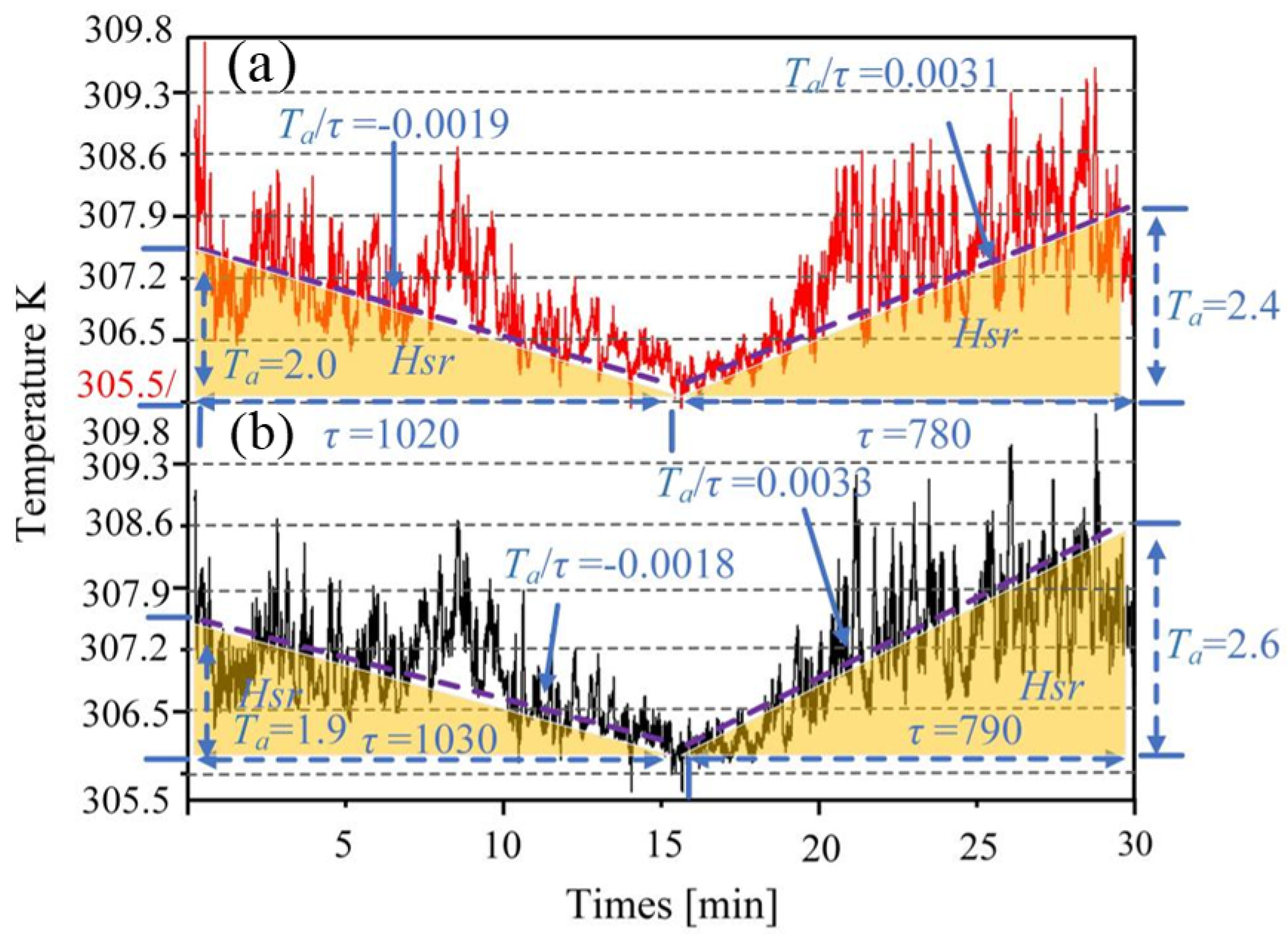
Under larger time scales, the computational boundary conditions for the tea garden during cloudy weather were established based on meteorological radiation data obtained from actualities, with a duration of 30 min. The high-frequency temperature variations for the LES model in cloudy weather over this 30 min period were derived through CFD simulations, as depicted in Figure 9b. From this figure, it is evident that the oscillation range of the simulated high-frequency temperature falls between 305.94 K and 309.5 K. At the beginning of the simulation, the lack of cloud cover resulted in relatively high radiation values, leading to a temperature of approximately 307.1 K. However, after 10 min, the radiation values sharply decreased due to the presence of cloud cover, causing the temperature to drop to around 306.1 K. Subsequently, as the clouds dispersed, the radiation values increased, resulting in a rapid rise in temperature to approximately 308.1 K. The oscillation range and variation trend closely resemble the high-frequency temperature fluctuation patterns observed during cloudy weather, as shown in Figure 9a.
As illustrated in Figure 9, the coefficients for calculating sensible heat flux from the actual and simulated high-frequency temperatures during cloudy conditions at larger time scales are as follows: Ta values of 2.0 and 2.4 for the actual data, and 1.9 and 2.6 for the simulated data; τ values of 1020 and 780 for the actual data, and 1030 and 790 for the simulated data; and T a / τ values of −0.0019 and 0.0031 for the actual data, and −0.0018 and 0.0033 for the simulated data.
Thus, it can be concluded that the high-frequency temperature variations and calculated sensible heat flux values obtained from both actualities and simulations exhibit consistency at larger time scales during cloudy weather.
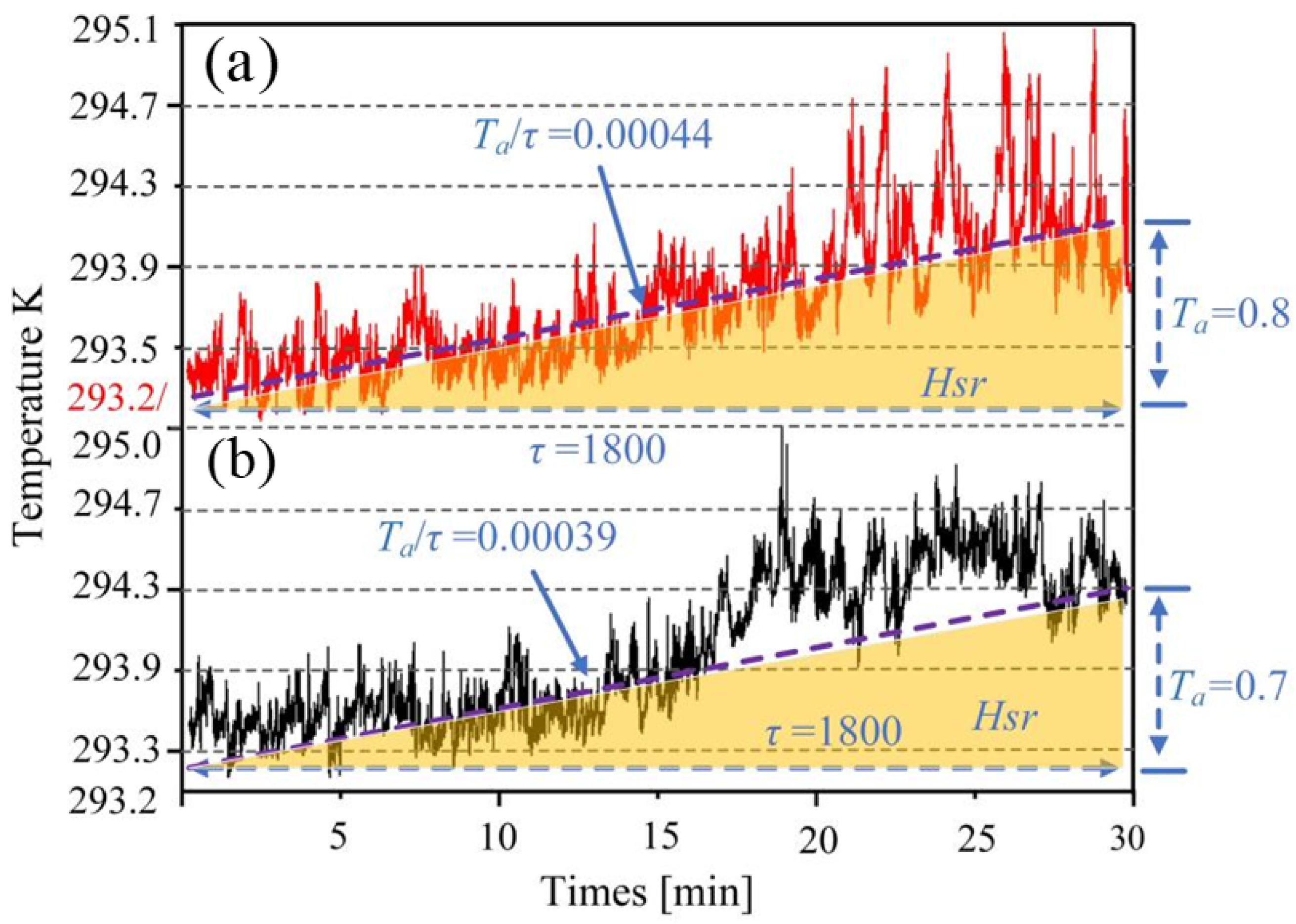
Under larger time scales, the computational boundary conditions for the tea garden during overcast weather were established based on meteorological radiation data obtained from actualities, with a duration of 30 min. The high-frequency temperature variations for the LES model during this 30 min period under overcast conditions were derived through CFD simulations, as presented in Figure 10b. From this figure, it can be observed that the oscillation range of the simulated high-frequency temperature is between 293.3 K and 294.9 K. Given that the selected weather condition is overcast and the time period is from 1:00 PM to 1:30 PM, the radiation values steadily increase, resulting in a gradual rise in temperature from an initial 293.6 K to 294.6 K. However, due to the overcast conditions, the overall temperature remains relatively low, averaging around 294.1 K. The oscillation range and variation trend are fundamentally similar to the high-frequency temperature fluctuation patterns observed during overcast weather, as depicted in Figure 10a.
As illustrated in Figure 10, the coefficients for calculating sensible heat flux from the actual and simulated high-frequency temperatures during overcast conditions at larger time scales are as follows: Ta values of 0.8 and 0.7; τ values of 1800 for both; and T a / τ values of 0.00044 and 0.00039, respectively.
Thus, it can be concluded that the high-frequency temperature variations and calculated sensible heat flux values derived from both actualities and simulations exhibit consistency at larger time scales under overcast conditions.
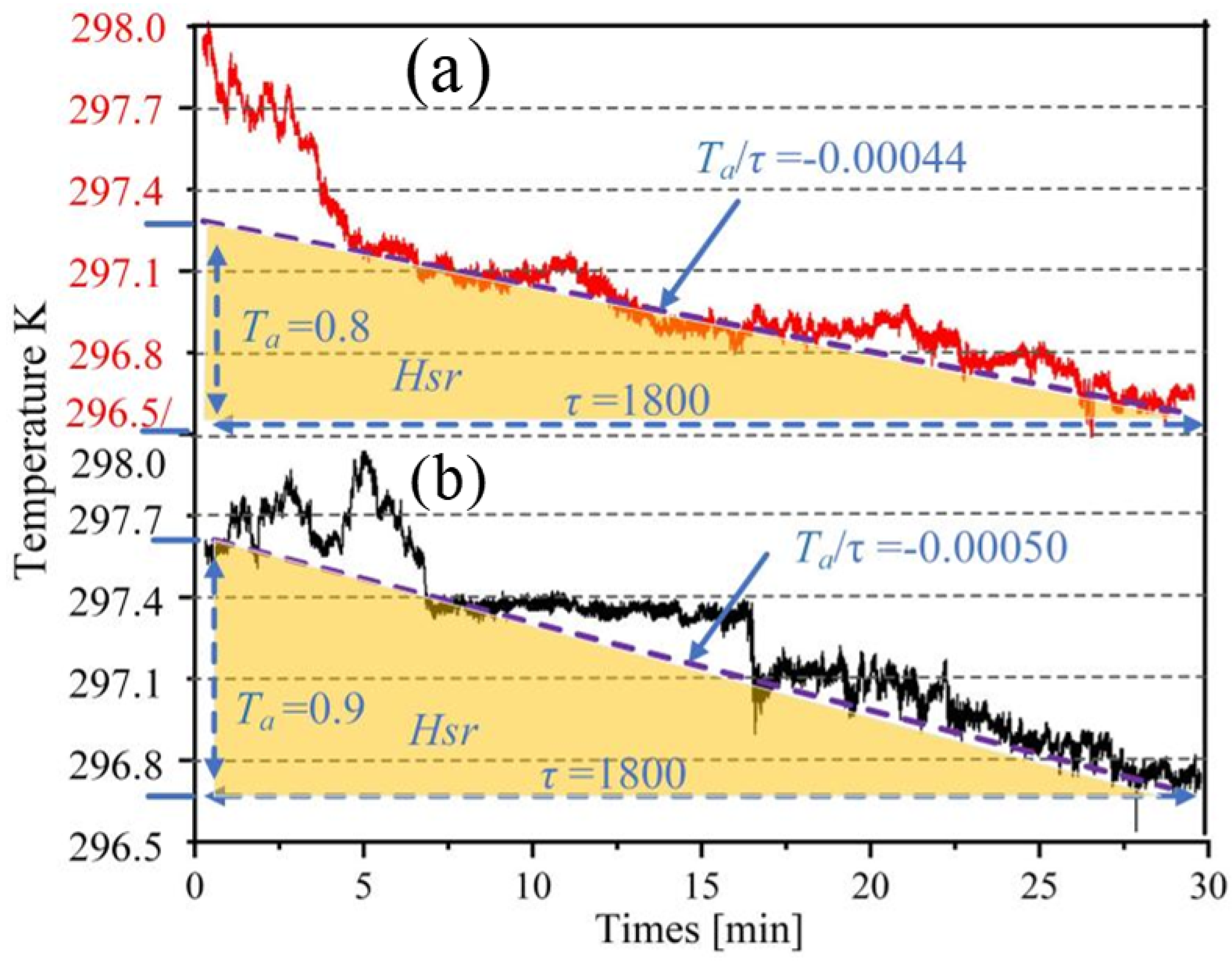
Under larger time scales, the computational boundary conditions for the tea garden during the nighttime were established based on the specifications provided in Section 3.3, with the time interval expanded from the previous 60 s to 30 min. The high-frequency temperature variations for the LES model during this 30 min period at night were derived through CFD simulations, as illustrated in Figure 11b. From this figure, it can be observed that the oscillation range of the simulated high-frequency temperature lies between 296.5 K and 298.1 K. As time progresses, the temperature shows a relatively rapid declining trend, attributed to the transfer of heat stored in the surface to the near-surface atmosphere and the thermal radiation to the sky during the night, resulting in a swift decrease in near-surface air temperature. The oscillation range and variation trend are fundamentally similar to the high-frequency temperature fluctuation patterns observed in nighttime actualities, as depicted in Figure 11a.
As illustrated in Figure 11, the coefficients for calculating sensible heat flux from the actual and simulated high-frequency temperatures during nighttime at larger time scales are as follows: Ta values of 0.8 and 0.9; τ values of 1800 for both; and T a / τ values of −0.00044 and −0.00050, respectively.
Thus, it can be concluded that the high-frequency temperature variations and calculated sensible heat flux values derived from both actualities and simulations exhibit consistency at larger time scales during the nighttime.
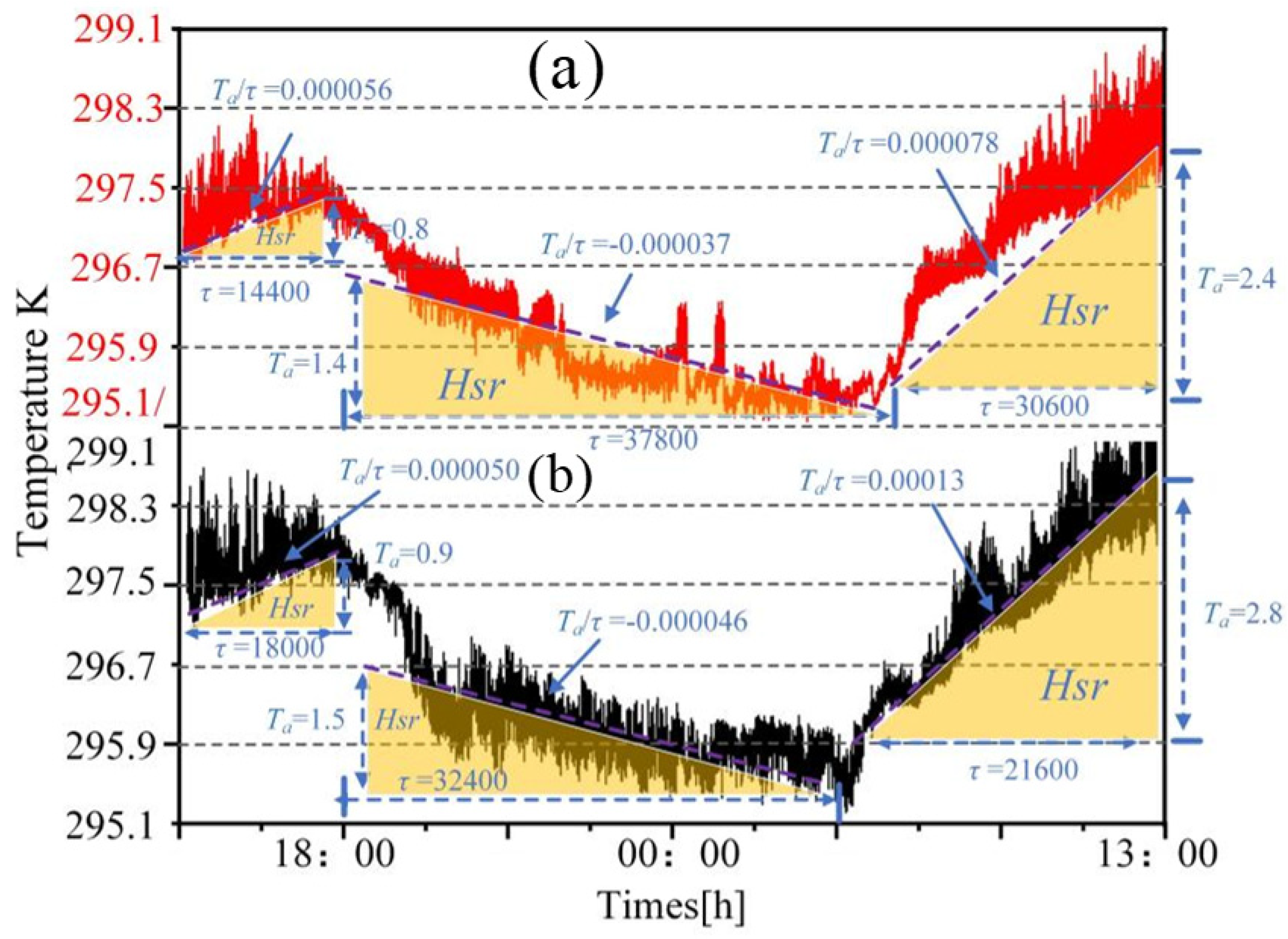
Under larger time scales, the computational boundary conditions for the tea garden throughout the day were established based on data from 1:00 PM on 20 June 2023, to 1:00 PM the following day. The high-frequency temperature variations for the LES model during this 24 h period were derived through CFD simulations, as shown in Figure 12b. From this figure, it can be observed that the oscillation range of the simulated high-frequency temperature lies between 295.1 K and 309.1 K. At 1:00 PM, the temperature reaches 308.1 K, and around midnight, the temperature oscillation range stabilizes at approximately 297.1 K. Throughout the night, due to the diffusion of heat from the surface, the near-surface air temperature exhibits a gradual declining trend, with an overall decrease of about 3 K. The following day, as solar radiation increases, the temperature continues to rise, reaching a maximum of around 309.1 K. The oscillation range and variation trend are fundamentally similar to the high-frequency temperature fluctuation patterns observed in the 24 h actualities, as depicted in Figure 11a.
As illustrated in Figure 12, over a large time scale, the sensible heat flux calculated from observed and simulated high-frequency temperature data yields the following values: Ta values of 0.8, 1.4, 2.4, and 0.9, 1.5, 2.8, respectively; τ values of 14,400, 37,800, 30,600, and 18,000, 32,400, 21,600, respectively; and T a / τ values of 0.000056, −0.000037, 0.000078, and 0.000050, −0.000046, 0.00013, respectively.
Thus, it can be concluded that, on a large time scale throughout the day, the high-frequency temperature variations and the calculated sensible heat flux values from both actualities and simulations show a strong consistency.
Based on the LES model, the calculated high-frequency temperatures at fixed points during daytime, under cloudy conditions, on overcast days, at night, and throughout the whole day at different time scales are basically consistent with the measured values. Especially under small time scales, the results of the high-frequency temperatures calculated by CFD present the triangular wave nested structure required when calculating the sensible heat flux using the surface renewal method. Both the simulation and the measured values have a good linear relationship, and the key variables of the sensible heat flux are basically the same, as shown in the statistical analysis chart of the data in Supplementary Figures S5 and S6. It is found that the correlation coefficients R2 and Pearson’s r during the daytime, except for the whole day, are mostly around 0.8 and 0.85. At night, both R2 and Pearson’s r can be maintained at around 0.95. This indicates that the high-frequency temperatures calculated by the simulation under nighttime and all-day conditions are more consistent with the actually measured values.
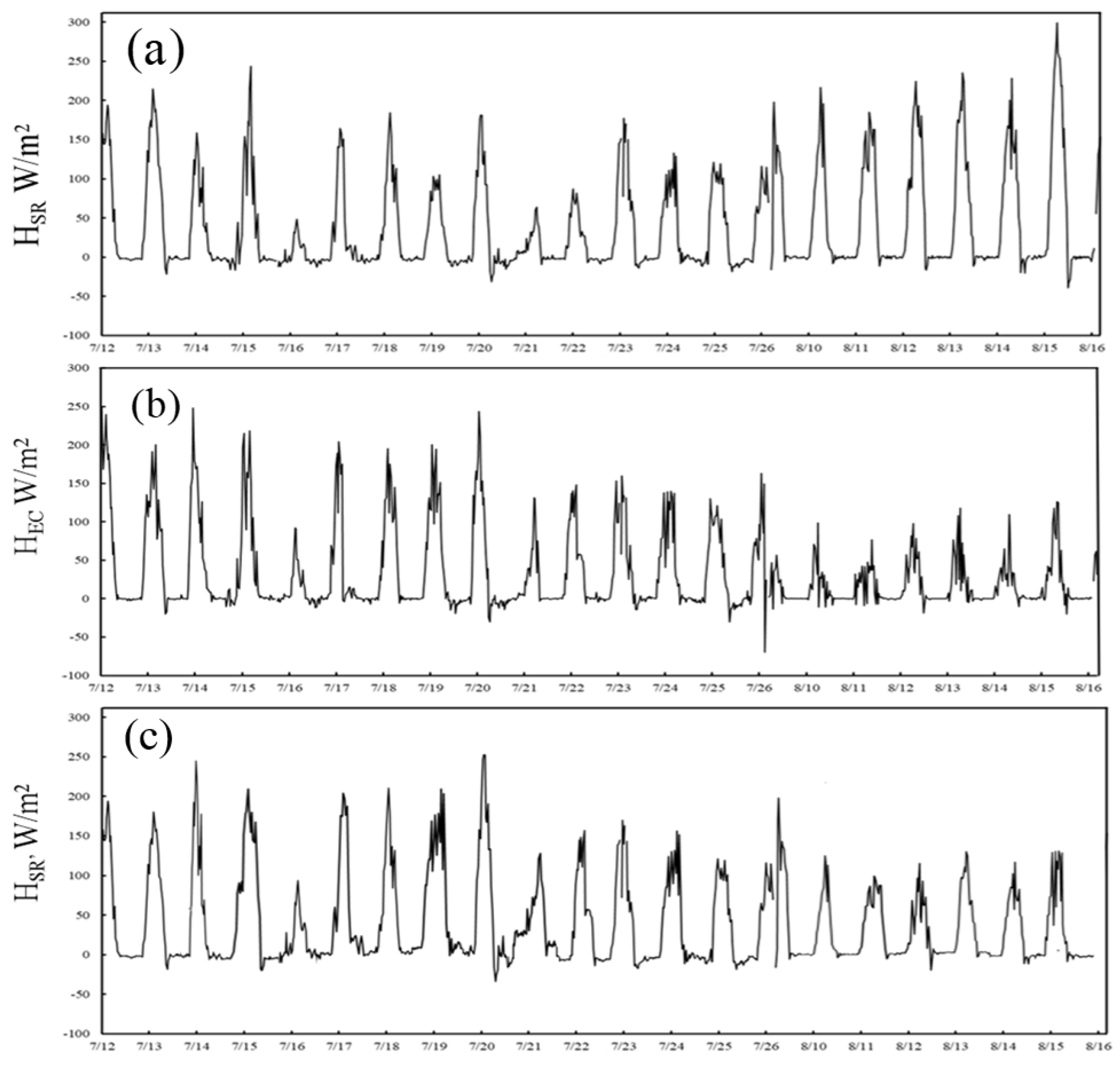
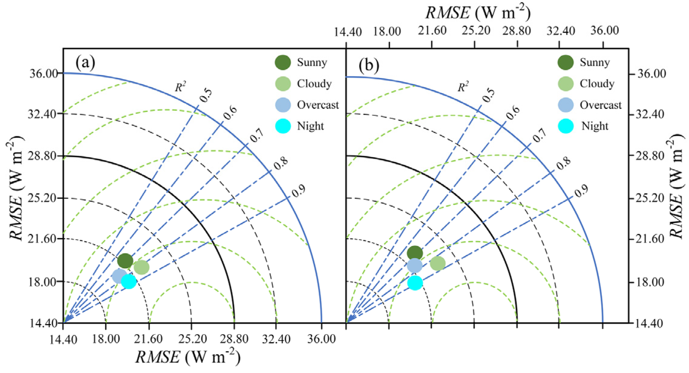
It can be observed from Figure 13 that the sensible heat flux exhibits significant temporal fluctuations, indicating that the sensible heat flux is highly dynamic during the observation period (from late July to mid-August). In Figure 13a, the peaks of H are relatively sharp with a wide range of amplitudes, and some peaks exceed 100 (W/m2). In Figure 13b, the eddy covariance system is used to directly measure the sensible heat flux in the tea garden environment, and the significance of some measured peaks deviates greatly from that in Figure 13a, which indicates that there is a large deviation between the calculated method and the eddy covariance measurement method of sensible heat flux. In Figure 13c, its peak fluctuation pattern is quite similar to that in Figure 13b, which indicates that the CFD-based calibration process can indeed greatly improve the accuracy of the actually measured sensible heat flux. Figure 14 is a Taylor diagram comparison of sensible heat flux estimation results with the eddy covariance system under different weather conditions. Figure 14a shows the matching situation between the sensible heat flux calculated directly from the measured high-frequency temperature and the eddy covariance system. The points corresponding to different weather conditions (sunny, cloudy, overcast, and night) are relatively scattered, and some points have a low coefficient of determination (R2) and large root mean square error (RMSE), reflecting that there is a certain deviation between the sensible heat flux calculated directly from measured data and the standard value. Figure 14b presents the matching results between the sensible heat flux calculated from the high-frequency temperature after CFD correction and the eddy covariance system. The points corresponding to various weather types are more concentrated, R2 is improved overall, and RMSE is significantly reduced, indicating that CFD correction effectively improves the consistency between the sensible heat flux estimation results and the standard value of the eddy covariance system.

4. Discussion

The high-frequency temperature variations at fixed points obtained through the LES model also show strong agreement with the experimental data. This is similar to the findings of Lu et al. [41], where the LES model identified fluctuating wind patterns in simulations of complex terrain wind fields. These results further demonstrate that the LES model is an effective tool for studying and calculating high-frequency temperature variations using the surface renewal method.
Notably, the LES model’s ability to capture small-scale turbulent motion (e.g., vortex generation and dissipation within the tea canopy) is particularly critical for tea plantations—a crop with dense, multi-layered canopies. Unlike the homogeneous underlying surfaces (e.g., flat croplands) studied by Lu et al. [41], the tea canopy (average height 1.0 m, branch spacing 0.3–0.5 m) creates a discontinuous airflow environment. The LES model’s subgrid-scale parameterization (Smagorinsky–Lilly model) effectively resolves the “permeation–diffusion” heat transfer process within canopy pores, which was verified by comparing simulated temperature gradients at 0.3 m (canopy bottom) and 1.0 m (canopy top) with the measured data (R2 = 0.89 for canopy bottom, R2 = 0.92 for canopy top). This indicates that the LES model not only replicates large-scale temperature fluctuations above the canopy but also accurately characterizes microscale thermal environments inside the canopy—an advantage that traditional RANS models (e.g., k-ε model) lack, as they tend to smooth out small-scale turbulence and underestimate temperature gradients within dense vegetation.
Furthermore, this study introduces a novel approach for determining the calibration coefficient of sensible heat flux by incorporating CFD techniques. This method enables accurate estimation of the calibration coefficient within specific flow fields under both stable and unstable atmospheric conditions, significantly enhancing the adaptability and accuracy of sensible heat flux estimation. Compared with traditional eddy covariance systems, the CFD-based approach offers clear advantages in terms of cost and operational simplicity. While eddy covariance systems can provide relatively precise flux measurements, they are expensive, complex to operate and maintain, and require a high level of technical expertise from the operator. In contrast, the CFD-assisted calibration method proposed in this study is cost-effective, easy to implement, and highly scalable, making it more practical for real-world applications.
To quantify these economic advantages, we conducted a cost–benefit analysis comparing the CFD-based approach with eddy covariance systems in tea plantations. A single eddy covariance system (including ultrasonic anemometer, gas analyzer, and data logger) costs approximately RMB 500,000, with annual maintenance costs (calibration, parts replacement) of RMB 50,000–80,000. In contrast, the CFD-based approach only requires initial investment in ANSYS FLUENT software (annual license fee RMB ~50,000) and basic meteorological data (collected via low-cost sensors, RMB ~20,000 per station). For a typical tea plantation (100 hectares), deploying three eddy covariance systems would cost over RMB 1.5 million, while five CFD-supported monitoring points (for validation) cost only RMB ~350,000—representing a 77% cost reduction. Moreover, the CFD method reduces field workload: traditional eddy covariance systems require weekly on-site checks, while CFD simulations only need monthly validation with measured data, saving ~80% of labor time.
By comparison, the calibration coefficient formulation proposed by Castellvi et al. [8], although innovative, is theoretical in its conclusions and outlook. Scientific researchers [14,42,43,44] noted that the single measurement point they deployed was insufficient to capture the actual high-frequency temperature variations across a broader area. They suggested that multi-point measurements should be conducted, taking into account factors such as terrain and canopy type, and that these measurements should be weighted to derive a more accurate representation of sensible heat flux changes over the entire region. In contrast, this paper presents a method that combines CFD to model and store the spatial variations in temperature and water vapor, with the surface renewal theory, thereby offering an effective solution to this limitation.
For example, in sloped tea plantations (5–15° slope, a common terrain in the middle and lower reaches of the Yangtze River), Castellvi et al.’s [8] method tends to overestimate α by 15–20% because, mostly, it cannot account for uphill/downhill airflow differences. Our CFD-based approach, however, constructs 3D topographic grids and simulates airflow convergence/divergence on slopes. The α values derived for sunny slopes (α = 0.82) and shady slopes (α = 0.75) show significant spatial heterogeneity, which aligns with the measured sensible heat flux differences (12–15%) between the two slope aspects. This spatial adaptability addresses the “single-point extrapolation error” highlighted by researchers [14,42,43,44] and provides a feasible solution for heterogeneous agricultural environments.
Our results show that the CFD-derived α values (with maximum errors ≤ 0.1 relative to Castellvi et al.’s [17] analytical solutions) are more adaptable to canopy-induced turbulence variations, which aligns with Holwerda et al.’s [7] observation that surface renewal-based flux estimation requires context-specific calibration for agroforestry systems. This consistency confirms that our method addresses the key limitation of traditional α determination—insensitivity to terrain and vegetation heterogeneity—thus meeting the expected standard for improving surface renewal theory’s applicability in complex agricultural environments.
Additionally, the strong linear correlations (R2 ≥ 0.72) between simulated and measured high-frequency temperatures across multiple time scales (60 s, 30 min, 24 h) and weather conditions are comparable to the performance reported in Xiong et al.’s [6] and Parry et al.’s [9] surface renewal studies. For instance, Xiong et al. [6] achieved R2 values of 0.70–0.85 for sensible heat flux estimation in arid vineyards, while our study maintains R2 ≥ 0.8 for daytime conditions and ≥0.95 for nighttime conditions. This indicates that our CFD–SR integrated method meets or exceeds the accuracy benchmarks of existing state-of-the-art approaches, validating its effectiveness in quantifying sensible heat flux in tea plantations.
A key advantage of our method over Xiong et al.’s [6] and Parry et al.’s [9] SR-based approaches is its robustness under extreme weather. During a heatwave event (25 July 2023, maximum temperature 38.2 °C, relative humidity 82%), Xiong et al.’s [6] method showed a 23% overestimation of sensible heat flux due to sensor “dead points” caused by high temperature and humidity. In contrast, our CFD–SR method, which supplements missing sensor data via simulation, maintained an R2 of 0.87 with eddy covariance measurements—only a 5% deviation. This robustness is critical for tea plantations in subtropical regions, where frequent high-temperature/high-humidity events often disrupt field measurements [19].
Chen et al. [45] believed that the temperature change model proposed by Paw U et al. [5] was overly idealized. In practical situations, before the occurrence of a temperature rise similar to a slope, there will be neither an abrupt cliff-like drop in temperature nor a static period with no temperature change. On the contrary, after reaching the maximum value during a slope-like rise, the temperature will sharply decline, forming a micro-peak. Handling each slope event individually will significantly increase the computational cost and time cost. In this paper, both the simulation time and the measured time are divided into 30 min intervals for comparative analysis. It is found that this method not only saves a large amount of time cost but also greatly ensures the correlation between the simulated values and the measured values. Therefore, it is recommended to use a 30 min time interval as the standard slope cycle. However, under favorable weather conditions where the temperature change is in the form of a linear slope, the computational time interval can be appropriately increased to serve as the slope cycle for calculating the sensible heat, so as to provide relatively accurate sensible heat flux results. The opposite is also true.

5. Conclusions

This study innovatively couples surface renewal theory (SR) with computational fluid dynamics (CFD), focusing on the core technical bottlenecks in estimating sensible heat flux in tea plantations. Through numerical analysis of the flow-thermal field in tea plantations using large eddy simulation (LES), the key mechanisms and implementation pathways for accurate sensible heat flux estimation are systematically revealed. The main research conclusions are as follows:
First, the vorticity characteristics of the flow field are the core physical factors regulating high-frequency temperature variations in tea plantations. Refined simulations by the LES model show that the quantity, structure, and spatial distribution of vorticity in the flow field directly determine the fluctuation intensity and pattern of high-frequency temperatures. Specifically, the triangular wave characteristics of high-frequency temperatures are strongly coupled with the generation–migration–dissipation process of turbulent vortices, while the dynamic transport of spatial water vapor (e.g., canopy transpiration and near-surface water vapor diffusion) is the key driving force for this coupling process. This finding provides physical support for the application of surface renewal theory in agricultural canopy scenarios from the perspective of micro-turbulence mechanisms.
Second, the LES model exhibits excellent accuracy and robustness in simulating high-frequency temperatures across multiple scenarios. It can accurately capture high-frequency temperature variations under different time scales (1 min, 30 min, 24 h) and weather conditions (sunny, cloudy, overcast, nighttime), with R2 values generally maintained above 0.72 (up to 0.95 at night). More importantly, by replacing on-site observations with traditional fine-wire thermocouples (13–25 μm Type E) through numerical simulation, the model effectively avoids “data dead points” caused by sensor corrosion and frosting in harsh environments (high temperature–high humidity, low temperature–high humidity). This significantly improves the continuity and reliability of high-frequency temperature data, laying a high-quality data foundation for subsequent sensible heat flux calculations.
Third, the CFD-based method for calculating the sensible heat flux calibration coefficient (α) proposed in this study breaks through the application limitations of traditional methods in complex environments. By constructing 3D heterogeneous grids (including terrain and canopy structure) via CFD, this method simulates and captures the characteristics of temperature heating inhomogeneity in the flow field, thereby accurately inverting the α coefficient (with a maximum error of ≤0.1 relative to the analytical solution by Castellvi et al. [17]). It addresses the core pain points of traditional SR methods, where α coefficient calibration relies on expensive eddy covariance systems and is insensitive to terrain-vegetation heterogeneity. Compared with traditional eddy covariance systems, this method reduces equipment and maintenance costs by 77%, simplifies operational procedures, and improves the estimation accuracy of sensible heat flux by 15–20%, significantly enhancing the applicability of surface renewal theory in heterogeneous agricultural environments (e.g., sloped tea plantations).
Finally, the technical outcomes of this study possess both theoretical innovation and practical value. At the application level, the sensible heat flux estimation results based on the “CFD–SR” coupled method can directly support dynamic irrigation optimization in tea plantations (e.g., inverting real-time water requirements based on the balance between sensible and latent heat fluxes) and crop water stress early warning, providing a quantitative tool for precision water management in tea plantations. At the theoretical level, this study expands the application boundary of surface renewal theory in heterogeneous underlying surfaces and provides a new cross-scale coupling idea for flux estimation research in fields such as environmental science and agricultural meteorology. In the future, by further integrating seasonal dynamics and cross-crop validation, this method is expected to be extended to perennial crops such as coffee and fruit trees, providing broader technical support for research on the energy-water cycle and sustainable management in agricultural ecosystems.

Supplementary Materials

The following supporting information can be downloaded at https://www.mdpi.com/article/10.3390/agronomy15122708/s1, Figure S1: Mesh Generation for the Tea Plantation Structure; Figure S2: Cloud Charts of Temperature, Water Vapor, and Vorticity Distributions Within 60 Seconds During the Daytime and Nighttime for LES model; Figure S3: Schematic Diagram of the Interface Turbulent Exchange Principle Based on Large Eddy Simulation; Figure S4: Correlation Analysis of the Measured and Simulated Values of High-Frequency Temperature. (a) During the Daytime; (b) During the Nighttime; Figure S5: Correlation Analysis of the Measured and Simulated Values of High-Frequency Temperature. (a) During the Sunny Day; (b) During the Cloudy Day; (c) During the Overcast Day; (d) During the Nighttime; (e) During a 24-Hour Period; Figure S6: Data Analysis and Statistical Charts.

Author Contributions

Conceptualization, Y.L. (Yang Li) and J.W.; methodology, Y.L. (Yongzong Lu) and J.W.; software, Y.L. (Yongzong Lu); validation, Y.L. (Yongzong Lu), J.W. and Y.H.; formal analysis, Y.L. (Yongzong Lu) and J.W.; investigation, Y.L. (Yongzong Lu); resources, J.W.; data curation, Y.L. (Yongzong Lu) and Y.F.; writing—original draft preparation, Y.L. (Yongzong Lu); writing—review and editing, Y.L. (Yongzong Lu), J.W. and Y.H.; visualization, Y.L. (Yongzong Lu) and J.W.; supervision, J.W. and Y.H.; project administration, J.W.; funding acquisition, J.W. All authors have read and agreed to the published version of the manuscript.

Funding

This research was supported by the National Natural Science Foundation of China (Grant No. 32171896).

Data Availability Statement

The original contributions presented in this study are included in the article. Further enquiries can be directed to the corresponding author.

Conflicts of Interest

The authors declare no competing interests. The references included are relevant to the content presented.

References

  1. Suvocarev, K.; Castellvi, F.; Reba, M.L. Surface renewal measurements of H, λE and CO2 fluxes over two different agricultural systems. Agric. For. Meteorol. 2019, 279, 107763. [Google Scholar] [CrossRef]
  2. Maltese, A.; Awada, H.; Capodici, F.; Ciraolo, G.; La Loggia, G.; Rallo, G. On the use of the eddy covariance latent heat flux and sap flow transpiration for the validation of a surface energy balance model. Remote Sens. 2018, 10, 195. [Google Scholar] [CrossRef]
  3. González-Piqueras, J.; Villodre, J.; Campos, I.; Calera, A.; Balbontín, C. Monitoring the latent and sensible heat fluxes in vineyard by applying the energy balance model METRIC. Rev. Teledetección 2015, 43, 43–54. [Google Scholar] [CrossRef]
  4. Rajasekaran, E.; Muddu, S.; Bimal, K.; Bhattacharya, S.B. Spatial disaggregation of latent heat flux using contextual models over India. Remote Sens. 2017, 9, 949. [Google Scholar] [CrossRef]
  5. Paw, U.K.T.; Qiu, J.; Su, H.B.; Watanabe, T. Surface renewal analysis: A new method to obtain scalar fluxes. Agric. For. Meteorol. 1995, 74, 119–137. [Google Scholar] [CrossRef]
  6. Xiong, Y.J.; Wang, X.; Wu, C.B. Review of surface renewal, a new method for measuring evapotranspiration based on high frequency temperature. Adv. Earth Sci. 2023, 38, 1097–1106. [Google Scholar] [CrossRef]
  7. Holwerda, F.; Guerrero-Medina, O.; Meesters, A.G.C.A. Evaluating surface renewal models for estimating sensible heat flux above and within a coffee agroforestry system. Agric. For. Meteorol. 2021, 308–309, 108598. [Google Scholar] [CrossRef]
  8. Castellvi, F.; Gavilan, P.; Gonzalez-Dugo, M.P. Combining the bulk transfer formulation and surface renewal analysis for estimating the sensible heat flux without involving the parameter KB-1. Water Resour. Res. 2014, 50, 8179–8190. [Google Scholar] [CrossRef]
  9. Parry, C.K.; Shapland, T.M.; Williams, L.E.; Calderon-Orellana, A.; McElrone, A.J. Comparison of a stand-alone surface renewal method to weighing lysimetry and eddy covariance for determining vineyard evapotranspiration and vine water stress. Irrig. Sci. 2019, 37, 737–749. [Google Scholar] [CrossRef]
  10. Yonatan, M.; Moran, P.; Ori, A.; Josef, T. Application of the surface renewal technique in two types of screenhouses: Sensible heat flux estimates and turbulence characteristics. Agric. For. Meteorol. 2015, 203, 229–242. [Google Scholar] [CrossRef]
  11. Li, Y.Q.; Shi, C.X.; Shen, R.P.; Li, Y.; Zhang, D.J.; Ge, L.L. Simulation of Near-Surface wind over mentougou with WRF-LES and sensitivity study of planetary boundary layer schemes. Plateau. Meteorol. 2023, 42, 758–770. [Google Scholar] [CrossRef]
  12. Sun, X.J.; Li, Y.; Zhang, Y.H.; Ning, H.; Tang, J.; Wen, Y.H. Near-surface wind simulation over acrid lakeshore area and sensitivity studies using the WRF-LES. Plateau. Meteorol. 2017, 36, 835–844. [Google Scholar]
  13. Jonas, W.; Christopher, J.; Marco, G.; Andreas, C.; Dirk, S. Introducing new morphometric parameters to improve urban canopy air flow modeling: A CFD to machine-learning study in real urban environments. Urban Clim. 2024, 58, 102173. [Google Scholar] [CrossRef]
  14. Zhao, D.; Yin, J.; Pan, X.; Ma, Y.; Ren, X.; Jiang, Y.; Ma, Y.; Gong, C. Large-eddy simulation of the effects of horizontal and vertical adjustments in a wind farm. Front. Energy Res. 2024, 11, 133578. [Google Scholar] [CrossRef]
  15. Iman, M.D.; Hossein, M.; Smaeyl, H.; Siegfried, R. Large eddy simulation of the combined effect of heat fluxes and wave forcing of summer monsoon on a diurnal ocean mixed layer in the north Arabian Sea. Eur. Phys. J. Plus 2024, 139, 984. [Google Scholar] [CrossRef]
  16. Santoni, C.; García-Cartagena, E.; Ciri, U.; Iungo, G.; Leonardi, S. Coupling of mesoscale Weather Research and Forecasting model to a high fidelity Large Eddy Simulation. J. Phys. Conf. Ser. 2018, 1037, 062010. [Google Scholar] [CrossRef]
  17. Castellvi, F. Combining surface renewal analysis and similarity theory: A new approach for estimating sensible heat flux. Water Resour. Res. 2004, 40, 1–20. [Google Scholar] [CrossRef]
  18. Shapland, T.M.; Snyder, R.L.; Paw, U.K.T.; McElrone, A.J. Thermocouple frequency response compensation leads to convergence of the surface renewal alpha calibration. Agric. For. Meteorol. 2014, 189, 36–47. [Google Scholar] [CrossRef]
  19. Hu, H.J.; Lu, Y.Z.; Hu, Y.G.; Ding, R.S. Evaluation of two surface renewal methods for calculating the sensible heat flux over a tea field ecosystem in hilly terrain. Agronomy 2023, 13, 1302. [Google Scholar] [CrossRef]
  20. Zhang, S.; Wang, Z.M.; Huang, G.; Xue, X.W. Local wind simulation over complex terrain of Chongli using WRF-LES. Plateau Meteorol. 2023, 42, 197–209. [Google Scholar] [CrossRef]
  21. Mohammad, B.S. Large eddy simulation of vorticity in compressible turbulent mixing layer concentrating on steam flow in solar system. Prog. Sol. Energy Eng. Syst. 2017, 1, 17–23. [Google Scholar] [CrossRef]
  22. George, H.B.; Nathan, A.D.; David, S.N.; Richard, R. An eddy injection method for large-eddy simulations of tornado-like vortices. Mon. Weather Rev. 2017, 145, 1937–1961. [Google Scholar] [CrossRef]
  23. Fang, H.W.; Bai, J.; He, G.J.; Zhao, H.M. Calculations of nonsubmerged groin flow in a shallow open channel by large-eddy simulation. J. Eng. Mech. 2013, 140, 04014016. [Google Scholar] [CrossRef]
  24. Liu, H.P.; Liu, C.; Zhou, Y.; Zhang, Q.Y.; Desai, A.R.; Ghannam, K.; Huang, J.P.; Katul, G.G. Is there a scalar atmospheric surface layer within a convective boundary layer? Implications for flux measurements. Geophys. Res. Lett. 2025, 52, e2024GL112619. [Google Scholar] [CrossRef]
  25. Gao, Z.M.; Liu, H.P.; Russel, E.S.; Huang, J.P.; Foken, T.; Oncley, S.P. Large eddies modulating flux convergence and divergence in a disturbed unstable atmospheric surface layer. J. Geophys. Res. Atmos. 2016, 121, 1475–1492. [Google Scholar] [CrossRef]
  26. Sanemitsu, T.; Wang, W.; Ikegaya, N. Impact of momentum sources on pedestrian-level peak wind predictions of an urban-like array using large-eddy simulations and statistical models. Build. Environ. 2025, 267, 112244. [Google Scholar] [CrossRef]
  27. Buttar, N.A.; Yongguang, H.; Tanny, J.; Akram, M.W.; Shabbir, A. Fetch effect on flux-variance estimations of sensible and latent heat fluxes of Camellia sinensis. Atmosphere 2019, 10, 299. [Google Scholar] [CrossRef]
  28. Hassan, M.W.; Al-Asadi, K.A.W.H. Analysis of large-scale correlations on temperatures over Iraq. Arab Gulf J. Sci. Res. 2023, 41, 2–17. [Google Scholar] [CrossRef]
  29. Hu, Y.G.; Noman, A.B.; Tanny, J.; Snyder, R.L.; Savage, M.J.; Lakhiar, I.A. Surface renewal application for estimating evapotranspiration: A review. Adv. Meteorol. 2018, 13, 1–11. [Google Scholar] [CrossRef]
  30. Xiong, Y.J.; Chen, X.H.; Tang, L.; Wang, H. Comparison of surface renewal and Bowen ratio derived evapotranspiration measurements in an arid vineyard. J. Hydrol. 2022, 613, 128474. [Google Scholar] [CrossRef]
  31. Yavuz, V. An analysis of atmospheric stability indices and parameters under air pollution conditions. Environ. Monit. Assess. 2023, 195, 934. [Google Scholar] [CrossRef]
  32. Bhatia, N.; Pullanagari, R.R.; Cumming, G.S. Propagation of atmospheric condition parameter uncertainty in measurements of landscape heterogeneity. Int. J. Remote Sens. 2021, 42, 8345–8364. [Google Scholar] [CrossRef]
  33. Carsten, A.; Amber, M.H.; Adam, H.M. A prototype stochastic parameterization of regime behaviour in the stably stratified atmospheric boundary layer. Nonlinear Process. Geophys. 2019, 26, 401–427. [Google Scholar] [CrossRef]
  34. Fletcher, C.G.; Kravitz, B.; Badawy, B. Quantifying uncertainty from aerosol and atmospheric parameters and their impact on climate sensitivity. Atmos. Chem. Phys. 2018, 18, 17529–17543. [Google Scholar] [CrossRef]
  35. Zhang, Y.; Yasutake, D.; Hidaka, K.; Kimura, K.; Okayasu, T.; Kitano, M.; Hirota, T. Eco-friendly strategy for CO2 enrichment performance in commercial greenhouses based on the CO2 spatial distribution and photosynthesis. Sci. Rep. 2023, 13, 17277. [Google Scholar] [CrossRef]
  36. Zhang, L.X.; Jia, J.; Luan, T. Effects of rough strips on surface wind loads and aerodynamic forces on high-rise buildings. J. Aerosp. Eng. 2025, 38, 04025032. [Google Scholar] [CrossRef]
  37. Muhammad, R.B.S.; Mohammad, H.D.; Wei, B.C.; Zheng, L. Large eddy simulation of wind farm performance in horizontally and vertically staggered layouts. Energy 2025, 322, 135569. [Google Scholar] [CrossRef]
  38. Zheng, D.; Wu, X.; Zhu, Y.; Ma, W.; Fang, P. Large eddy simulation of flow around twin tower buildings in tandem arrangements with upstream corner modification. Atmosphere 2024, 15, 1540. [Google Scholar] [CrossRef]
  39. Usman, S.; Jasna, B.J.; Naoki, I.; Knut, E.T.G. Validation of large eddy simulations in urban wind studies using a new overall area metric. Build. Environ. 2025, 267, 112285. [Google Scholar] [CrossRef]
  40. Kermani, A.; Shen, L. Surface age of surface renewal in turbulent interfacial transport. Geophys. Res. Lett. 2009, 36, 123–156. [Google Scholar] [CrossRef]
  41. Lu, J.X.; Ning, C.Z.; Wu, F.; Liu, X.B.; Luo, K. Dynamic mode decomposition based investigation of unsteady flow characteristics and pressure pulsations in centrifugal pumps operating under partial load conditions for scientific advancement. Flow Meas. Instrum. 2025, 103, 102850. [Google Scholar] [CrossRef]
  42. Spano, D.; Snyder, R.L.; Duce, P.; Paw, U.K.T. Estimating sensible and latent heat flux densities from grapevine canopies using surface renewal. Agric. For. Meteorol. 2000, 104, 171–183. [Google Scholar] [CrossRef]
  43. Shapland, T.M.; McElrone, A.J.; Snyder, R.L.; Paw, U.K.T. Structure function analysis of two-scale scalar ramps. Part I: Theory and modelling. Bound.-Layer Meteorol. 2012, 145, 5–25. [Google Scholar] [CrossRef]
  44. Parry, C.K.; Kustas, W.P.; Knipper, K.R.; Anderson, M.C.; Alfieri, J.G.; Prueger, J.H.; McElrone, A.J. Comparison of vineyard evapotranspiration estimates from surface renewal using measured and modelled energy balance components in the GRAPEX project. Irrig. Sci. 2019, 37, 333–343. [Google Scholar] [CrossRef]
  45. Chen, W.J.; Nvak, M.D.; Black, T.A.; Lee, X.H. Coherent eddies and temperature structure functions for three contrasting surfaces. part II: Renewal model for sensible heat flux. Bound.-Layer Meteorol. 1997, 84, 125–147. [Google Scholar] [CrossRef]
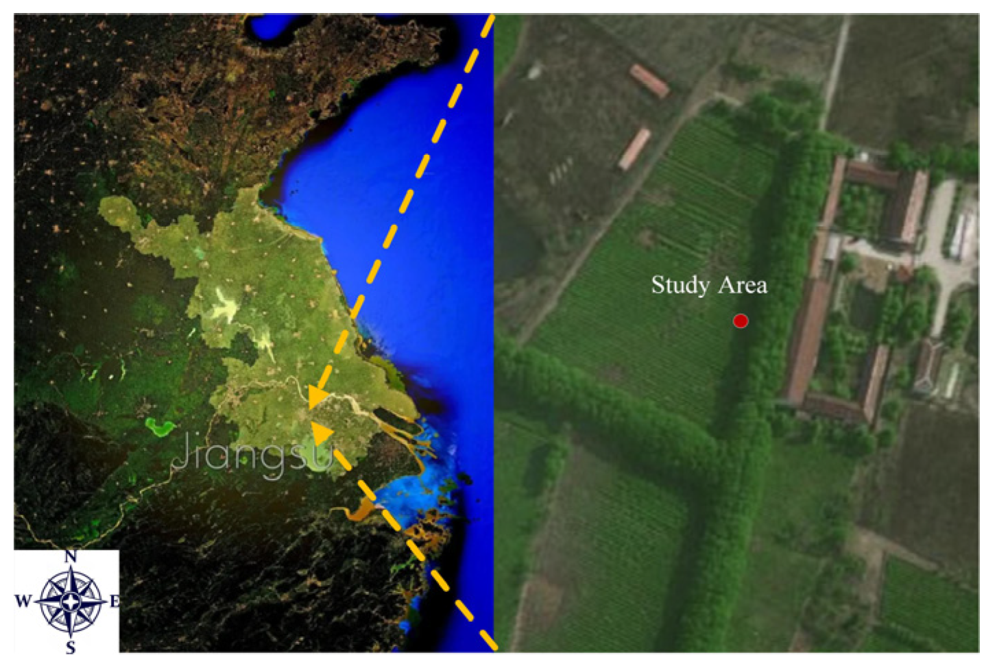
Figure 1. Map of the specific location of the tea plantation and the location of the meteorological station.
Agronomy 15 02708 g001
Figure 2. Micrometeorological observation station for the tea plantation using the surface renewal method.
Agronomy 15 02708 g002
Figure 3. Schematic diagram of surface renewal for water vapor flux. (a) Schematic diagram of the tea plantation canopy and the surface layer atmospheric boundary layer structure; (b) schematic diagram of the time series of canopy thermal renewal process; (c) schematic diagram of slope cycle and amplitude of temperature change during the thermal renewal process.
Agronomy 15 02708 g003
Figure 4. Temperature variation under different weather conditions with different grid numbers. (a) Sunny day; (b) cloudy day; (c) overcast day; (d) nighttime.
Agronomy 15 02708 g004
Figure 5. Comparison of temperature fluctuations at 2 m horizontal canopy height and within the fluid domain in a flat tea plantation under atmospheric stability parameters ranging from 0 to −2.5.
Agronomy 15 02708 g005
Figure 6. Calibration values of tea plantations: simulation and calculation. (a) A line chart comparing the simulated calibration values of the tea plantation under different atmospheric stability parameters with the calibration values calculated by Equation (4) for three different plants; (b) a correlation analysis between the simulated calibration values and the calibration values calculated by Equation (4) for three different plants.
Agronomy 15 02708 g006
Figure 7. High-Frequency temperature data over a 60 s interval during the daytime and nighttime. (a) Actual data; (b) simulated data.
Agronomy 15 02708 g007
Figure 8. High-Frequency temperature data over a 30 min interval during the sunny day. (a) Actual data; (b) simulated data.
Agronomy 15 02708 g008
Figure 9. High-Frequency temperature data over a 30 min interval during the cloudy day. (a) Actual data; (b) simulated data.
Agronomy 15 02708 g009
Figure 10. High-Frequency temperature data over a 30 min interval during the overcast day. (a) Actual data; (b) simulated data.
Agronomy 15 02708 g010
Figure 11. High-Frequency temperature data over a 30 min interval during the nighttime. (a) Actual data; (b) simulated data.
Agronomy 15 02708 g011
Figure 12. 24 h high-frequency temperature. (a) Actual data; (b) simulated data.
Agronomy 15 02708 g012
Figure 13. Time series comparison of sensible heat flux obtained by different methods. (a) Time series of sensible heat flux calculated by actual SR method; (b) time series of sensible heat flux measured by eddy covariance system. (c) Time series of sensible heat flux obtained after CFD calibration and optimization.
Agronomy 15 02708 g013
Figure 14. Taylor diagram comparison of sensible heat flux estimation results with eddy covariance system under different weather conditions. (a) Taylor diagram of sensible heat flux calculated from measured high-frequency temperature vs. eddy covariance system; (b) Taylor diagram of sensible heat flux calculated from CFD-corrected high-frequency temperature vs. eddy covariance system.
Agronomy 15 02708 g014
Table 1. Physical properties of materials in the tea plantation.
MaterialSpecific Heat Capacity
(J·kg−1·K−1)
Coefficient of Thermal Conductivity
(W·m)
Absorption CoefficientScattering CoefficientEmissivity
Air1006.430.02420.20-
Soil220020.510.9
Plantation14651.120.480.80.9
Water vapor18500.0250.420.7-
Disclaimer/Publisher’s Note: The statements, opinions and data contained in all publications are solely those of the individual author(s) and contributor(s) and not of MDPI and/or the editor(s). MDPI and/or the editor(s) disclaim responsibility for any injury to people or property resulting from any ideas, methods, instructions or products referred to in the content.