Article

Projection of Land Use and Habitat Quality Under Climate Scenarios: A Case Study of Arid Oasis Urban Agglomerations

1
State Key Laboratory of Geohazard Prevention and Geoenvironment Protection, Chengdu University of Technology, Chengdu 610059, China
2
College of Geography and Planning, Chengdu University of Technology, Chengdu 610059, China
*
Author to whom correspondence should be addressed.
Agronomy 2025, 15(12), 2704; https://doi.org/10.3390/agronomy15122704
Submission received: 25 September 2025 / Revised: 16 November 2025 / Accepted: 20 November 2025 / Published: 24 November 2025
(This article belongs to the Section Agroecology Innovation: Achieving System Resilience)

Abstract

Understanding the evolutionary dynamics of land use and habitat quality (HQ) under climate change scenarios is pivotal for formulating science-based biodiversity conservation policies and promoting climate-resilient urban development in arid regions. By integrating the SD–PLUS–InVEST framework with SPEI-driven drought scenarios, this study introduces a novel coupling mechanism that links climate variability, land-use transitions, and HQ evolution in the Northern Slope of the Tianshan Mountains (UANSTM) under SSP–RCPs scenarios. The HQ assessment was validated using the Remote Sensing Ecological Index (RSEI). Simultaneously, the Optimal Multivariate-Stratification Geographical Detector (OMGD) was applied to identify scale-optimized drivers of HQ changes. The results indicated the following: (1) From 2000 to 2020, cultivated and construction land in the UANSTM expanded, while forest and water areas declined, with unused land remaining dominant from 2000 to 2020. (2) HQ decreased from 0.36 to 0.33 (2000–2020), significantly correlating with RSEI (Pearson r = 0.329, Spearman ρ = 0.446, p < 0.001), with climatic, vegetation, and coupled natural-social factors remaining the dominant drivers. (3) From 2020 to 2050, under all climate scenarios, the areas of farmland, grassland, and construction land are expected to grow, while HQ is projected to improve through the conversion of low-quality areas into moderate- and high-quality habitats (greatest under SSP119, least under SSP585). The framework advances predictive insights for arid-region ecological planning, supporting practical applications in habitat management and sustainable land-use planning, while providing a methodological paradigm for dryland habitat resilience assessment.

1. Introduction

Habitat quality (HQ) is widely recognized as a key indicator for evaluating biodiversity conservation, as it reflects how effectively an ecosystem can maintain species populations and sustain their reproductive capacity [1,2]. Nevertheless, the combined pressures of intensifying climate variability and expanding human disturbances have reshaped habitat configurations [3,4], leading to fragmentation and degradation that exacerbate habitat vulnerability and further threaten ecological integrity, agricultural productivity, and socioeconomic resilience [5,6,7]. Habitat fragmentation reduces landscape connectivity among habitat patches, disrupts energy flows and material cycles, and weakens ecosystem stability and service provision [8], thereby affecting agricultural production, water regulation, and climate stability, ultimately diminishing the capacity of socioeconomic systems to cope with external disturbances [9], particularly in dryland ecosystems [10]. Moreover, climate change can reconfigure environmental carrying capacity and erode region-specific ecological distinctiveness, further altering patterns of land-use suitability and exacerbating systemic risks [11,12]. In light of these mounting pressures, assessing the temporal and spatial variations in HQ and land use is vital for advancing regional biodiversity conservation and informing sustainable land management strategies.
International research on HQ spans several key areas, including examinations of the interrelationships between HQ and other ecosystem services [13], as well as the construction of ecological security networks based on HQ assessments [14]. For example, Ashrafi et al. [15] examined multiple ecosystem services, including HQ, in the Zarrinehrud River Basin (Iran) and simulated their dynamics under future climate scenarios. Similarly, Polasky et al. [16] quantified changes in ecosystem services, biodiversity habitat, and landowner returns resulting from land-use changes in Minnesota. Among the tools employed, the InVEST model has been extensively adopted for HQ evaluation owing to its straightforward implementation and effective visualization outputs [17]. The habitat quality component of the model, which is driven by land-use information, operates on the premise that human-induced land-use activities diminish habitat quality and pose risks to regional biodiversity [18]. However, most existing applications focus on the spatial patterns generated by model outputs, whereas systematic validation against real ecological conditions remains limited. For example, Luo et al. [19] only applied the InVEST model to analyze the spatiotemporal characteristics of HQ in shrinking cities, without further validation against field observations. This limitation restricts the model’s applicability for ecological management and spatial planning purposes.
Dryland ecosystems, which are inherently fragile, have experienced exacerbated ecological deterioration facing the joint impacts of climate change and human activities [20,21]. Consequently, in recent years, there has been growing attention to ecosystem services in arid regions, including HQ [22,23], with numerous studies focusing on how these services respond under various changing scenarios, such as development policies and climate change [24,25,26]. The Coupled Model Intercomparison Project Phase 6 (CMIP6) integrates Shared Socioeconomic Pathways (SSPs) and Representative Concentration Pathways (RCPs) to construct a range of representative future scenarios, widely used in climate and ecological impact assessments [25,27,28,29]. A growing body of research now focuses on forecasting land-use patterns under SSP-RCP scenarios while concurrently examining the potential future dynamics of ecosystem services [30]. Among these studies, the most commonly applied method is the integration of the System Dynamics (SD) model with the Patch-generating Land Use Simulation (PLUS) model. For instance, Sui et al. [31] integrated the SD-PLUS model with the InVEST model to simulate land-use and land-cover changes in the Ili River Valley under varying climate scenarios and to evaluate the spatiotemporal dynamics of habitat quality. By combining the strengths of SD model in modeling socioeconomic evolution with the spatial capabilities of the PLUS model, this framework enables integrated predictions regarding land-use amounts and their spatial patterns. In this framework, SD model predicts the demand for different land-use types based on socioeconomic drivers such as population, GDP, which are then fed into PLUS to allocate land types spatially, considering neighborhood effects, transition probabilities, and patch generation rules. Iteratively coupling SD outputs with PLUS spatial simulations across multiple time steps allows the framework to capture interactions between socioeconomic evolution and landscape dynamics [24,30,31,32]. However, existing simulation frameworks often overlook a key constraint in arid ecosystems—drought—when constructing future scenarios, limiting their applicability in such regions. To address this gap, this study incorporated the Standardized Precipitation–Evapotranspiration Index (SPEI) into the SD model to quantify drought-induced variations in land use demand, thereby explicitly integrating drought dynamics into the simulation of land use change. Notably, in this study, the driving factors of the InVEST-HQ model are derived from land use–based human disturbances, which serve as static inputs. In contrast, the SPEI does not directly drive the HQ module but is embedded into the SD–PLUS system through the land use demand component, influencing habitat quality indirectly by altering land use structure and intensity.
On the other hand, identifying and quantifying drivers of HQ can provide critical insights into the relative contributions of climate variability and land use change to habitat degradation or improvement. Nevertheless, prevailing approaches frequently employ arbitrarily selected spatial scales, leaving the optimal scales for key drivers insufficiently quantified [33]. The Optimal Multivariate-Stratification Geographical Detector model integrates factor discretization optimization and scale detection into the traditional geographical detector [34]. Accordingly, the model is employed in this study to investigate the driving factors of HQ changes at optimal spatial scales.
The Urban Agglomeration on the Northern Slope of the Tianshan Mountains (UANSTM), located deep within the Eurasian continent and far from oceanic moisture transport, experiences low precipitation, an arid climate, and fragile ecosystems, making it one of China’s representative dryland urban clusters [21]. Moreover, the region’s complex topography and diverse vegetation types contribute to its rich biodiversity, which is simultaneously threatened by drought stress and human activities. In recent years, as a key hub of the Silk Road Economic Belt, the UANSTM has undergone rapid urbanization and industrialization, leading to significant shifts in land use patterns that may profoundly impact HQ and ecosystems. Given its dual vulnerability to climatic drought and anthropogenic pressure, the UANSTM provides an ideal case for exploring how land-use dynamics and drought variability jointly influence HQ in arid urban systems. Therefore, this study aims to (1) develop an integrated SD–PLUS–InVEST framework coupled with the SPEI to simulate land use and HQ dynamics in the UANSTM under multiple scenarios; (2) analyze the spatiotemporal evolution of HQ and validate the results using the Remote Sensing Ecological Index (RSEI); (3) identify the dominant drivers and scale-dependent interactions influencing HQ changes to support ecological security and sustainable development in arid regions. This research provides a scientific basis for understanding the coupled effects of drought and land use on habitat quality, offering valuable insights for biodiversity conservation and regional sustainability in arid ecosystems.
Based on existing studies and the characteristics of the study region, we hypothesize that the following:
H1: 
Future land use is expected to be dominated by the expansion of cropland, grassland, and built-up areas, with a decrease in unused land area of ≥5%.
H2: 
The overall regional habitat quality (HQ) is projected to improve, with the HQ index expected to increase by ≥5%.
H3: 
Under different climate change scenarios, the reduction in unused land and the increase in grassland are anticipated to largely explain the future changes in HQ.

2. Materials and Methods

2.1. Study Area

The Urban Agglomeration on the Northern Slope of the Tianshan Mountains in Xinjiang (UANSTM) is geographically situated between 83°26′~91°54′ E and 41°11′~46°12′ N, bounded by the Gurbantünggüt Desert to the north and the Tianshan Mountains to the south. This ecotone harbors strategic resource endowments, serves as a critical node along the China–Central Asia–West Asia Economic Corridor, a strategic artery of the Belt and Road Initiative (Figure 1). The region encompasses a total area of approximately 215,400 km2, accounting for 13% of the total land area of Xinjiang Uygur Autonomous Region. UANSTM exhibits a temperate continental climate regime, characterized by a mean annual temperature of 7.5 °C and a precipitation regime averaging 185.34 mm/yr. Dominant vegetation assemblages comprise drought-adapted steppe grasslands and xerophytic shrubs. Under the dual forcing of anthropogenic activities and natural climatic variability, this region manifests pronounced salinization along oasis peripheries, accelerated glacial retreat, and urbanization-driven land transformation that incurs compounded pressures on land resource allocation, oasis degradation, and environmental vulnerabilities arising from fragmented ecological networks. The ecological fragility of the UANSTM poses severe constraints on regional socioeconomic sustainability.

2.2. Data Source

The data framework of this study comprises two main categories: geospatial datasets and socioeconomic statistical indicators (Table 1).
The geospatial datasets include the following: (1) Land Use/Land Cover (LULC) (2000–2020), sourced from the Resource and Environmental Science Data Center, Chinese Academy of Sciences (https://www.resdc.cn/). Both the LULC data and the datasets applied in the PLUS v1.40 model were converted to a 100 m spatial resolution via bilinear interpolation to improve computational efficiency while maintaining spatial accuracy. (2) The natural climate data in CMIP6 were obtained from the National Tibetan Plateau Science Data Center, China. This dataset is based on the latest SSP scenarios released by the IPCC (SSP119, SSP245, SSP585), with each scenario including climate data from three GCMs (EC-Earth3, GFDL-ESM4, MRI-ESM2-0). After preprocessing and Delta resampling, 1 km monthly mean temperature and precipitation data for China under multiple scenarios and models were obtained [35]. In this study, the temperature and precipitation data from the MRI-ESM2-0 climate model were used.
The socioeconomic statistical indicators include the following: (1) inputs for the SD model, such as population, gross domestic product (GDP), fixed asset investment, aquatic product demand, grain demand, and area of cultivated land converted to forest, which were derived from the Xinjiang Statistical Yearbook (2000–2020), China. (2) CMIP6 Socioeconomic Scenario Data, including projected population, GDP, mean annual temperature, and mean annual precipitation under different SSPs, which were obtained from the Science Data Bank [36].

2.3. Methodology

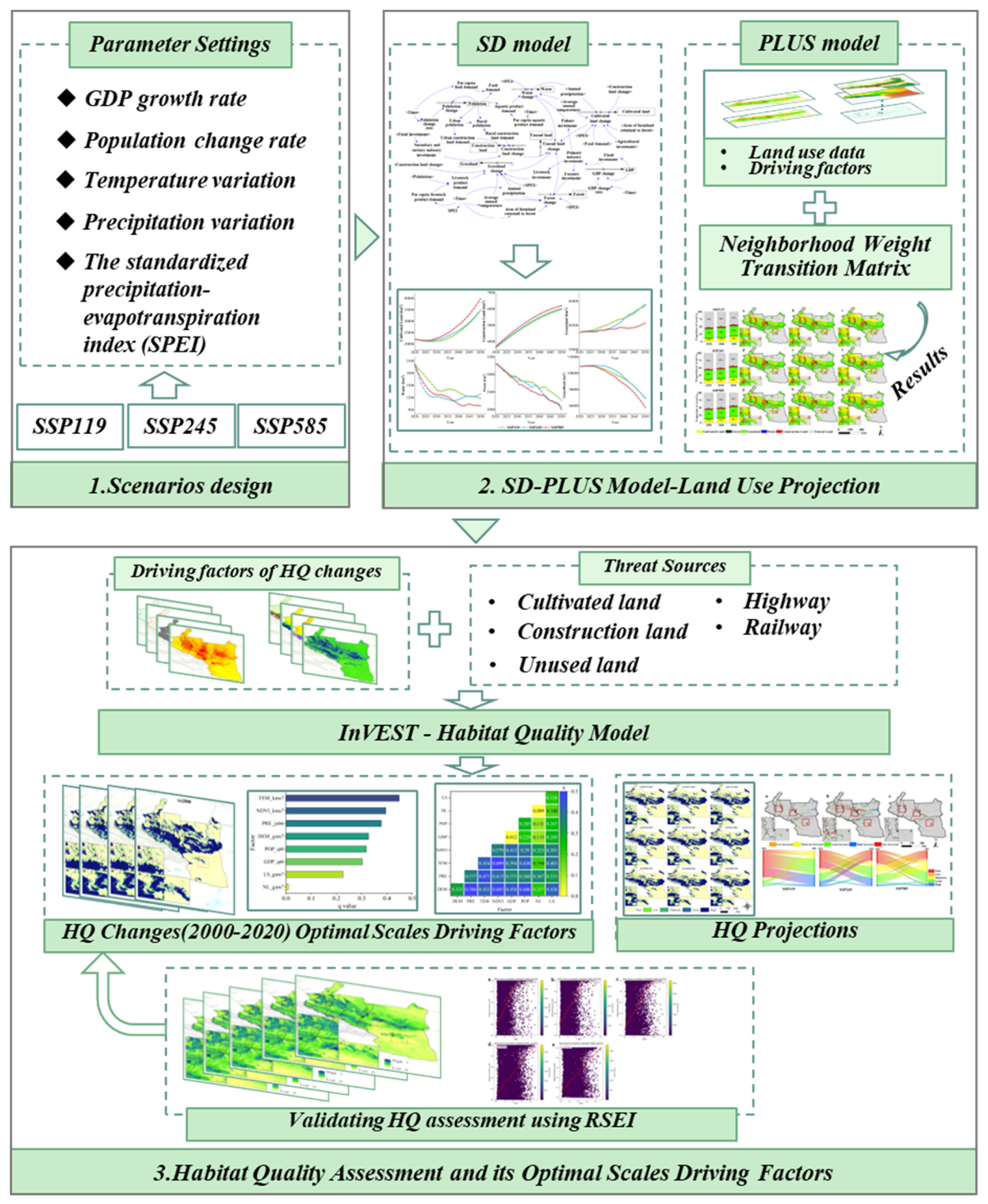
This study aims to forecast the evolution of HQ in arid regions under the combined influence of future climate change—particularly drought variability—and human activities (Figure 2). To this end, an SD-PLUS model integrated with a drought index was constructed to project land-use dynamics in the UANSTM across multiple scenarios. Subsequently, the InVEST model was applied to evaluate HQ changes from past to future, with the RSEI used to validate the reliability of the InVEST results. Finally, the OMGD model was utilized to uncover the key drivers of HQ variations at the optimal spatial scale. These results offer a scientific basis for informed ecological planning and sustainable management in arid ecosystems.

2.3.1. The Standardized Precipitation-Evapotranspiration Index (SPEI)

The Standardized Precipitation-Evapotranspiration Index (SPEI) was employed to characterize projected drought dynamics within the UANSTM under future climate change scenarios. The SPEI at different timescales represents distinct types of drought [37]. SPEI-01 (1 month) reflects short-term drought, SPEI-03 (3 months) and SPEI-06 (6 months) capture seasonal wetness and dryness variations, and SPEI-12 (12 months) represents long-term drought trends and interannual variability [38,39]. Since other SD model inputs are annual data, SPEI-12 was selected as the drought indicator and incorporated into the SD model in a table function to simulate long-term drought scenarios in the study area. The classification of drought severity based on SPEI levels is presented in Table A1. The SPEI-12 values for the period 2000–2050 were obtained through standardized normalization of the climatic water balance (precipitation minus potential evapotranspiration, PET) [28]. PET was calculated using the Hargreaves method, which estimates evapotranspiration using only minimum and maximum air temperatures, thereby providing a simplified computational approach [40]. Its accuracy and applicability have been widely validated across diverse climatic regimes [41].

2.3.2. Climate Scenario Framework Derived from CMIP6 Datasets

The CMIP6 framework integrates Shared Socioeconomic Pathways (SSPs) and Representative Concentration Pathways (RCPs) to elucidate the causal links between socioeconomic development and climate outcomes through radiative forcing dynamics [29,42]. The SSP-RCP coupled scenarios enhance projections of anthropogenic pathways by capturing interdependencies between socioeconomic structures and emission constraints [24]. Three representative scenarios—SSP119, SSP245, and SSP585—were employed to simulate the socioeconomic-emission nexus. Specifically, SSP119 represents a sustainable and low-carbon development pathway characterized by low greenhouse gas emissions, slow population growth, and proactive ecological protection efforts [43]. SSP245 describes a moderate forcing scenario that reflects balanced economic growth, moderate population increase, and emission trajectories consistent with historical development patterns [42]. In contrast, SSP585 depicts a high forcing scenario dominated by fossil fuel-intensive development, rapid population expansion, and accelerated urbanization [24,44]. Building on this framework, a multidisciplinary parameterization system was established to quantify land-use demand under coupled drought climate scenarios (Table A2). This system systematically integrates five key drivers—Gross Domestic Product (GDP), Population (POP), Temperature, Precipitation, and SPEI.

2.3.3. System Dynamics Model

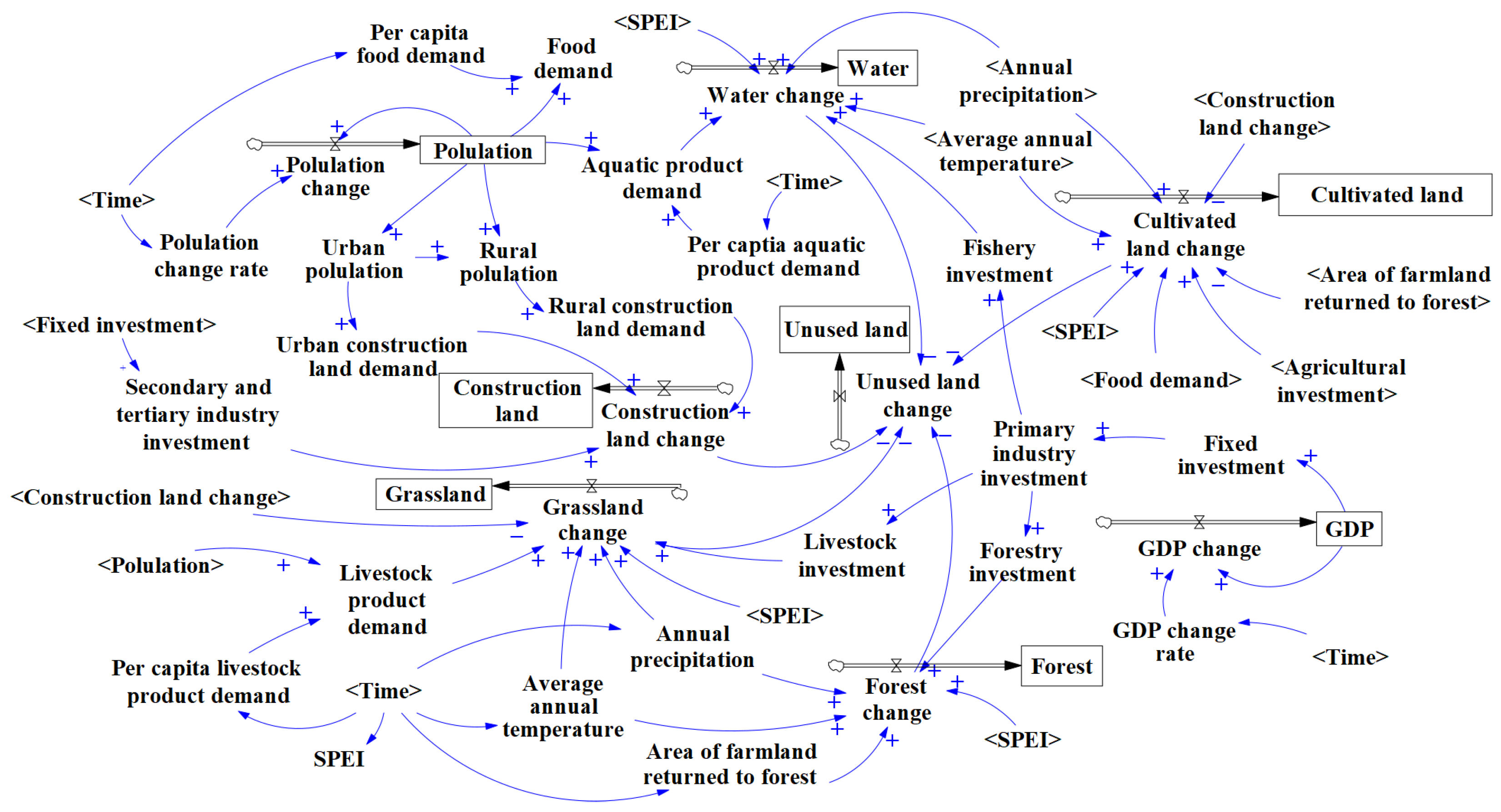
The System Dynamics (SD) model effectively captures nonlinear causal loops within multi-feedback hierarchies [45]. Building upon previous studies [30,46], this study employed the Vensim PLE 10.2.2 platform to simulate annual system dynamics from 2000 to 2050 (Figure 3). It comprises four interconnected subsystems—economic, demographic, climatic, and land use—parameterized through causal loop diagrams to simulate cross-scale interactions under scenario-driven perturbations. In the economic subsystem, GDP variations influence investment in the agro-industrial complex (agriculture, forestry, fishery, husbandry, and construction), regulating land-use demand–supply equilibria. The demographic subsystem captures demand for agro-pastoral commodities and urban–rural population shifts, indirectly driving land-use transitions. The climate subsystem captures the long-term effects of precipitation, temperature variability, and drought on agricultural lands, grasslands, forested regions, and aquatic systems. Specifically, variations in these climatic factors modulate the demand coefficients for forest, cultivated land, grassland, and water, thereby indirectly influencing land-use patterns across the study region. The land-use subsystem models the aggregate dynamics of distinct land-use categories.
To evaluate the structural robustness of the model, this study conducted a sensitivity analysis on 10 key parameters within the SD model. Specifically, each parameter was increased or decreased by 10% annually, and the effects of these changes on the main state variables were assessed [46]. The results show that the average sensitivity of all 10 primary variables is below 1 (Table A5), indicating that the model is insensitive to parameter perturbations. These findings demonstrate that the land-use demand system constructed in this study exhibits good stability and reliability under parameter variations.

2.3.4. PLUS Model

The PLUS model effectively identifies the driving forces behind land expansion and predicts land use patterns [47,48]. Fourteen geospatial drivers encompassing natural and socioeconomic dimensions were systematically incorporated into the PLUS model: Digital Elevation Model (DEM), slope, mean annual temperature, annual precipitation, GDP, population density, soil type, and proximity metrics to highways, railways, hierarchical road networks, county administrative centers, and rivers. Neighborhood weight factors are closely related to the formation of land-use types [49]. Wang et al. [50] selected relevant landscape indices at both the landscape and patch levels to examine spatial pattern relationships and their transformation dynamics, thereby revealing the expansion intensity of different land-use types. Furthermore, this study employs their computational formula (Equation (1)) to calculate domain weights based on historical data from the UANSTM. The neighborhood coefficients for distinct land-use categories and scenario-configured transition matrices within the UANSTM are systematically tabulated in Table A6. Additionally, to ensure predictive robustness, the spatial distribution of land use in 2020 was simulated based on the 2010 land use data. Diagnostic validation was conducted by comparing the simulated results with the actual 2020 land use, and the model’s accuracy was quantitatively assessed using the Kappa coefficient.
X = X m i n m a x m i n
In the equation, X denotes the domain weight of a specific land-use type, m i n represents the minimum area among the six land-use types, and m a x represents the maximum area among them.

2.3.5. InVEST—Habitat Quality Model

HQ serves as a critical indicator of ecosystem biodiversity status. The Habitat Quality module within the InVEST modeling framework is recognized as one of the most scientifically robust and widely adopted methodologies for systematic HQ assessment in ecological research [32]. The HQ patterns in the UANSTM were systematically quantified through the application of the InVEST-HQ module. Five anthropogenic disturbance proxies were identified as primary threat sources in this investigation, including cultivated land, construction land, unused land, highways, and railways. These land-use types are directly linked to varying intensities of human interference with natural ecosystems. Cultivated land and construction land represent zones of concentrated human activity, exerting substantial pressure on ecological processes through land development and agricultural expansion. Major transportation corridors (highways and railways) further amplify habitat fragmentation and facilitate human access across landscapes. In contrast, unused land, characterized by low vegetation cover and degraded environmental conditions, contributes to ecological vulnerability and reduced habitat quality. Therefore, these five land-cover types were selected to comprehensively capture the dominant anthropogenic threats to the regional ecological environment [51,52]. The relevant parameters of each threat factor were obtained according to the InVEST technical documentation and the relevant literature [21,22,31], details are shown in Table 2 and Table 3.
To assess the robustness of the HQ results derived from the InVEST model, this study performed a sensitivity analysis by varying the weights of the threat factors and the decay distances by ±10% (Table A7). The results showed that the HQ values obtained under parameter perturbations were extremely highly correlated with the baseline results (Pearson’s r = 0.9999–1.0000; RMSE < 0.005), indicating that the evaluation outcomes are largely insensitive to plausible parameter variations. Therefore, the HQ results obtained from the InVEST model in this study are robust and reliable.

2.3.6. Validating HQ Using Remote Sensing Ecological Index (RSEI)

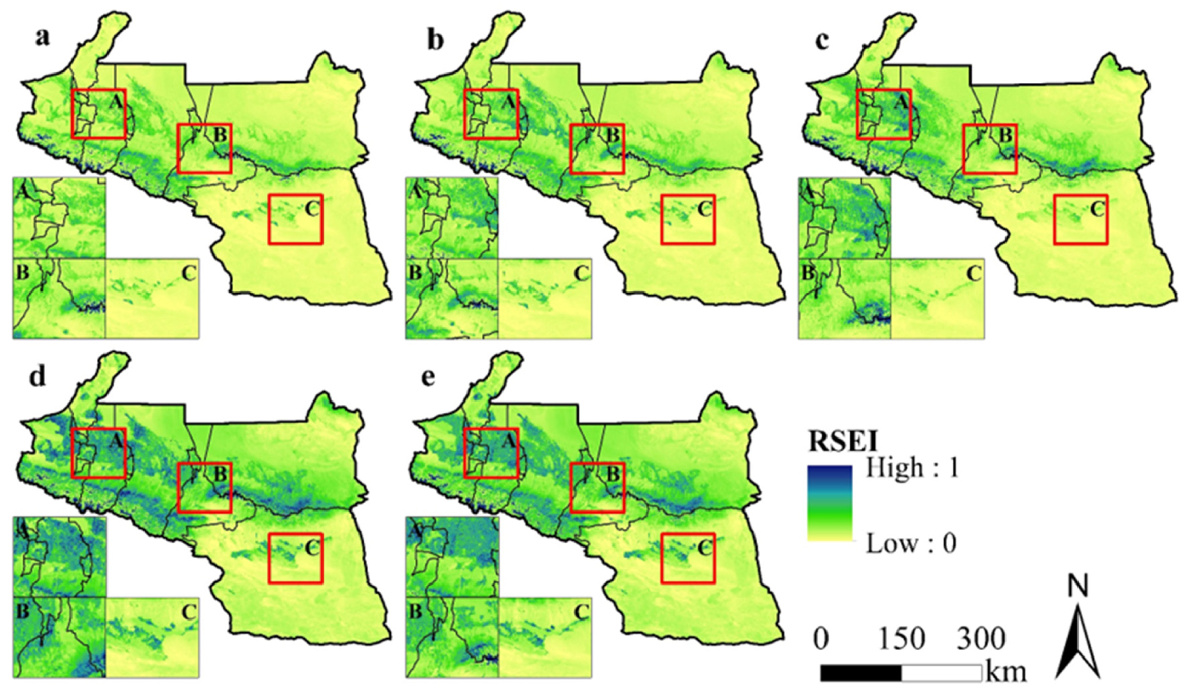
To ensure that the HQ derived from land-use data accurately reflects the ecological status of the UANSTM, the remote sensing ecological index (RSEI) was calculated for the region from 2000 to 2020 using Google Earth Engine (GEE), a cloud-based geospatial processing environment that enables efficient handling of large-scale datasets without the constraints of traditional local computing [53]. Subsequently, correlation analysis was conducted to examine the relationship between the RSEI and HQ.

2.3.7. Optimal Multivariate-Stratification Geographical Detector Model

The Optimal Multidimensional-stratification Geographical Detector (OMGD) model, developed by Guo et al., enhances the traditional geographical detector by integrating factor discretization optimization and scale detection. The discretization optimization module automatically evaluates multiple classification strategies (e.g., equal interval, quantile, and natural breaks) and selects the scheme that maximizes the q-statistic, thereby minimizing subjectivity and improving the explanatory power of spatial stratified heterogeneity (SSH). Meanwhile, the scale detector identifies the optimal spatial scale for SSH analysis [34]. This dual optimization enables the OMGD model to more accurately capture both single-factor and multi-factor interactions in complex geographical processes [54]. This study employed the OMGD model to comprehensively investigate the driving factors influencing HQ in the UANSTM from 2000 to 2020. A multiscale grid system (1000 m, 1500 m, 2000 m, 2500 m, 3000 m, and 3500 m) was constructed to examine scale-dependent ecological determinants of HQ. Furthermore, the factor stratification optimization procedure was applied to identify the most suitable discretization methods for the explanatory variables, ensuring robust and reliable model performance.
Driving factors were selected across natural environmental and socioeconomic dimensions, encompassing: Gross Domestic Product (GDP), population density (POP), nighttime light intensity (NL), livestock density (LS), digital elevation model (DEM), normalized difference vegetation index (NDVI), annual precipitation (PRE), and mean annual temperature (TEM).

3. Results

3.1. Spatiotemporal Dynamics and Scenario-Based Projections of LULC Transformation

3.1.1. Historical Transition of Land Use

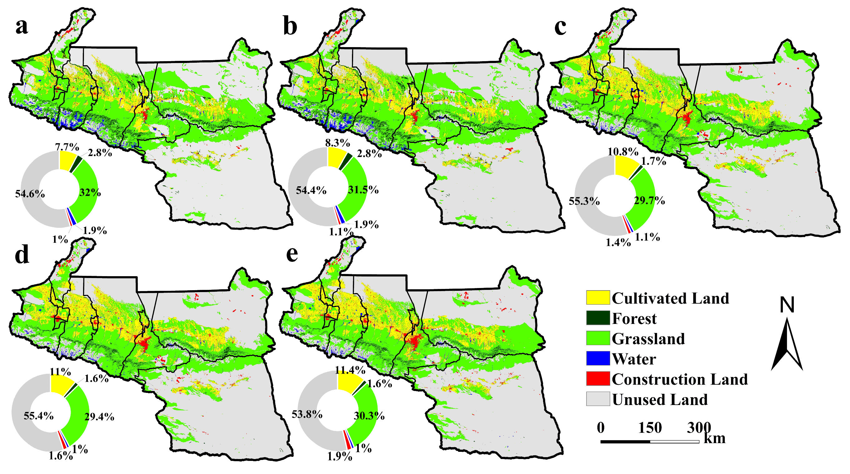
The land-use composition of the UANSTM was dominated by unused land, followed by grassland and cultivated land, while forest, water, and construction land occupying a minor proportion (Figure 4). Between 2000 and 2020, the region experienced significant land-use changes, including the expansion of cultivated and construction land, alongside the degradation of forest and water areas. Specifically, cultivated land and construction land expanded by 3.7% and 0.9%, respectively, while forest area decreased by 2422 km2 over 2000–2020. Grassland initially contracted but later recovered, with a notable 1181.37 km2 gain from 2010 to 2020. Linear regression trend significance tests for each land-use type (Table A8) further indicate that both cultivated land and construction land experienced significant increases from 2000 to 2020 (p < 0.0197 and p < 0.0012, respectively); meanwhile, forest and water areas declined significantly (p < 0.0452 and p < 0.0505, respectively). Unused land, the dominant land cover, showed a biphasic transition—first expanding, then contracting—but still accounted for over 50% of the study area. Its distribution was concentrated in Turpan City and Changji Hui Autonomous Prefecture.

3.1.2. Land-Use Projections

A comparative accuracy assessment was conducted between the simulated output and the actual land-use map, yielding an overall classification accuracy of 93.38%, a Kappa coefficient of 0.89 and an FoM value of 0.9761. A Kappa value greater than 0.8 indicate that the simulation results are reliable and the model accuracy is statistically satisfactory [7]. The relative error between the predicted and actual areas of each land-use type was within 1% (Table A4), statistically validating that the coupled SD-PLUS framework is highly reliable in simulating land-use patterns under drought conditions.
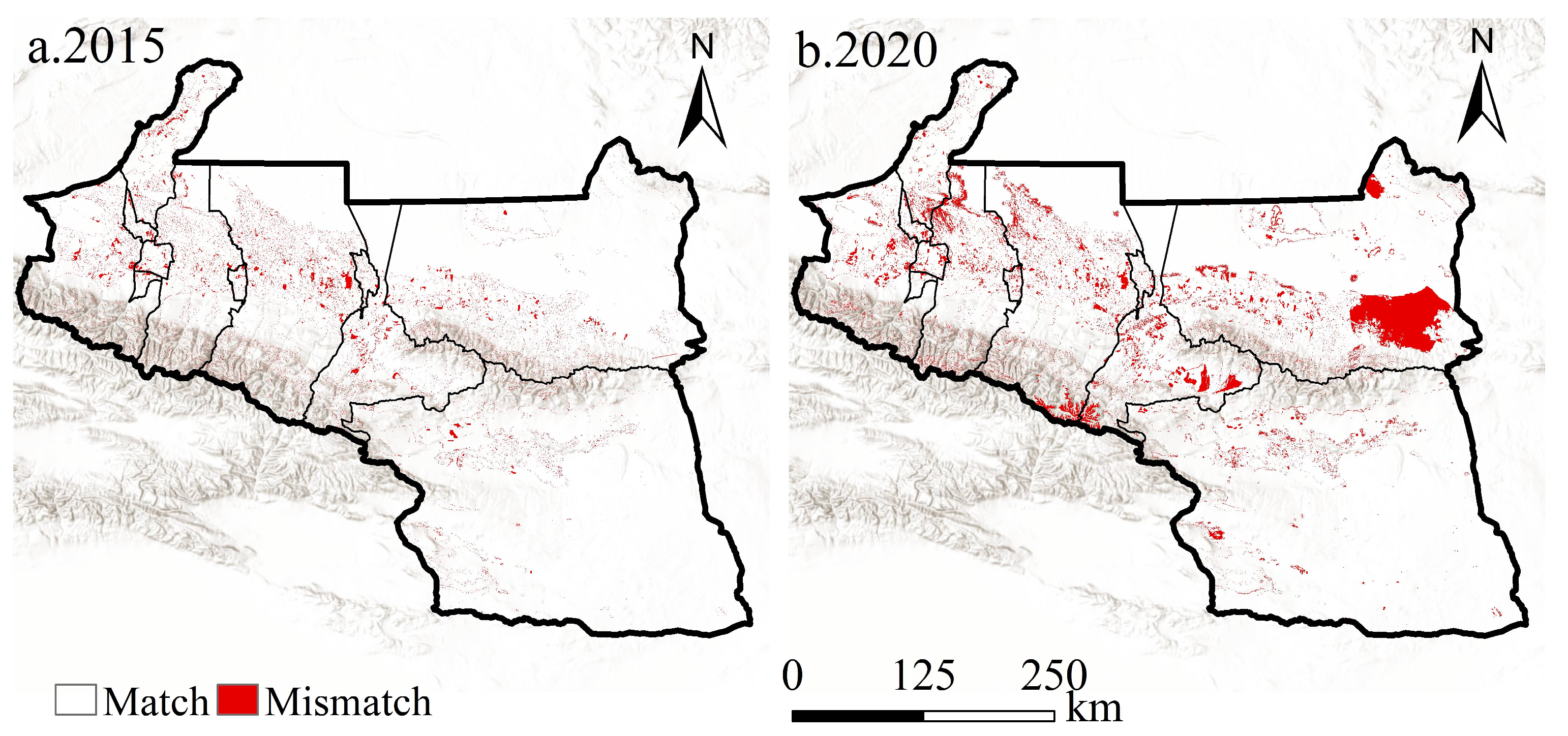
Moreover, to further evaluate the spatial predictive capability of the PLUS model beyond conventional accuracy metrics, this study used 2010 as the baseline year to simulate the land-use distributions for 2015 and 2020, and it constructed spatial disagreement maps between the simulated and actual land-use patterns (Table A9, Figure A1). Specifically, the actual land-use maps for each period were compared with the corresponding simulated maps on a pixel-by-pixel basis. Pixels exhibiting inconsistent land-use types between the two maps were assigned a value of 1, whereas consistent pixels were assigned 0, thereby generating spatial disagreement layers for each period. These disagreement maps provide an intuitive depiction of land-use transitions across the study area, highlight high-change zones that the model must capture. The result showed that the spatial disagreement is predominantly concentrated in areas with intense land-use transitions, particularly where frequent conversions occur among desert, grassland, and cropland. These high-change zones indicate that the PLUS model faces greater uncertainty when capturing neighborhood-driven land-use dynamics. In contrast, regions dominated by forest, construction land and water bodies exhibit very low disagreement, suggesting that the model can effectively reproduce the spatial stability of these landscape types. Overall, the spatial disagreement maps provide a more spatially explicit perspective for evaluating model performance, demonstrating that the PLUS model performs reliably in stable landscapes, whereas its accuracy is relatively limited in areas undergoing rapid transformation.
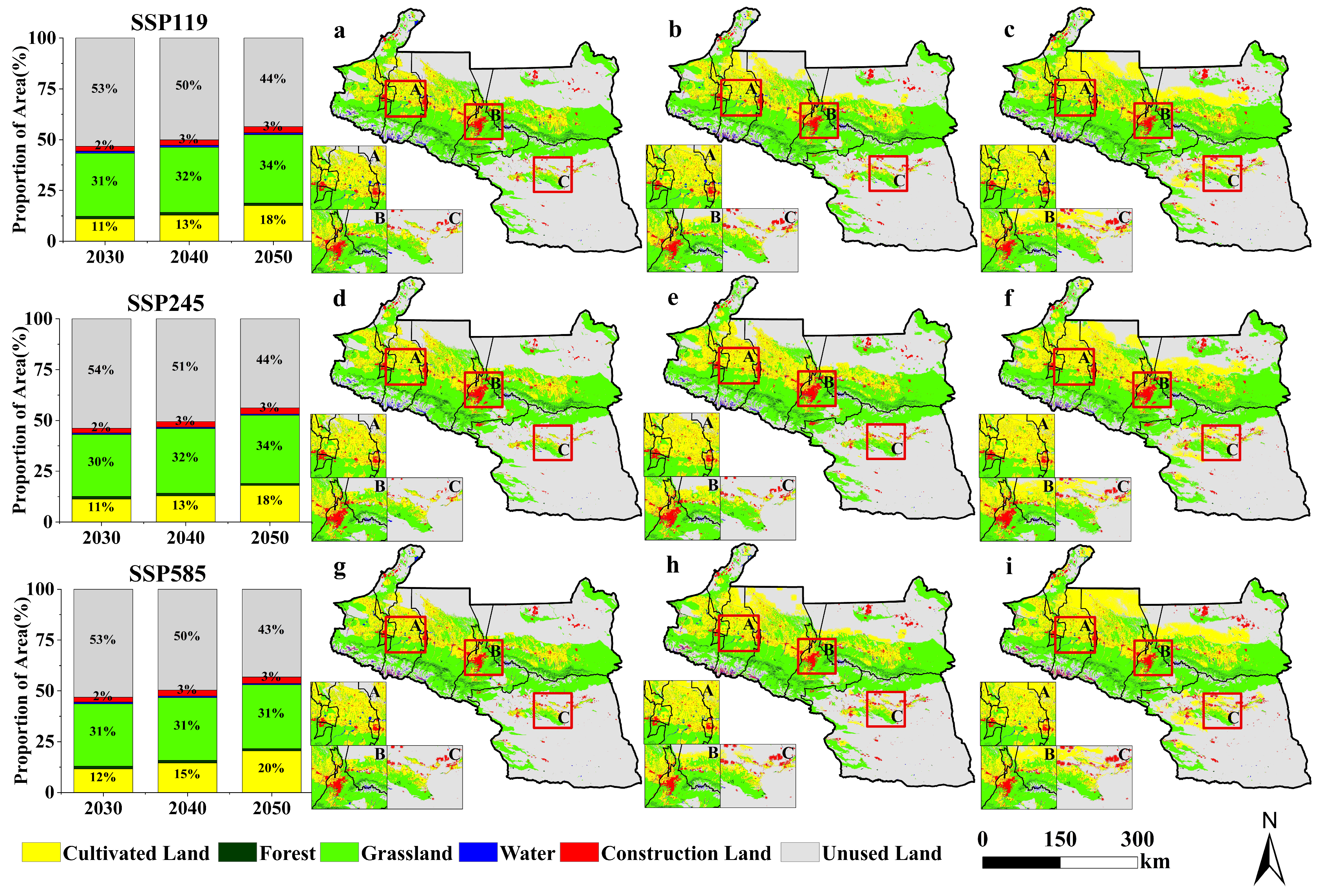
The scenario-based simulations indicate consistent land-use transition patterns across all three SSPs. Cultivated land, construction land, and grassland are projected to continue expanding, whereas forest, water, and unused land are expected to decline (Figure A2 and Figure 5, Table A10). Under the SSP119, a partial conversion of cultivated land to grassland is projected (1551.58 km2), along with a marginal increase in construction land (378.55 km2). Under the SSP245, a notable conversion of 4396.97 km2 from grassland to cultivated land is projected. Under the SSP585, accelerated expansion of cultivated and construction land may lead to varying degrees of forest and water loss. It is important to note that, to maintain model tractability and ensure comparability with previous SD-PLUS applications, explicit irrigation water demand, groundwater availability, and basin-scale water-budget constraints were not incorporated. Consequently, the simulated expansion of cultivated and construction land represents potential spatial trajectories driven by land demand and suitability conditions, rather than water-feasible development pathways.
Across the three climate scenarios during 2020–2050, unused land is predicted to be predominantly converted to other land-use categories, with clear transition trends toward cultivated land, grassland, and construction land. Specifically, under the SSP119 scenario, unused land is projected to be converted to cultivated land, grassland, and construction land, covering 14,058.02 km2, 3402.37 km2, and 1349.50 km2, respectively. Under the SSP245 scenario, the largest conversion of unused land is anticipated to occur to cultivated land, totaling 11,188.81 km2. Under the SSP585 scenario, the area of unused land converted to cultivated land is expected to reach 17,138.12 km2, while 1245.55 km2 will be transformed into construction land. Overall, compared with 2020, the proportion of unused land is expected to decrease by approximately 9.8% across these three scenarios. Spatiotemporal analysis further revealed that cultivated land will primarily cluster and expand primarily within northern subregions, including Shawan City, Changji Hui Autonomous Prefecture, and Turpan City. In contrast, grassland and construction land are expected to exhibit expansion around the periphery of existing urban and agricultural centers.

3.2. Habitat Quality and Spatial Distribution Characteristics

3.2.1. Validating HQ Assessment Using RSEI

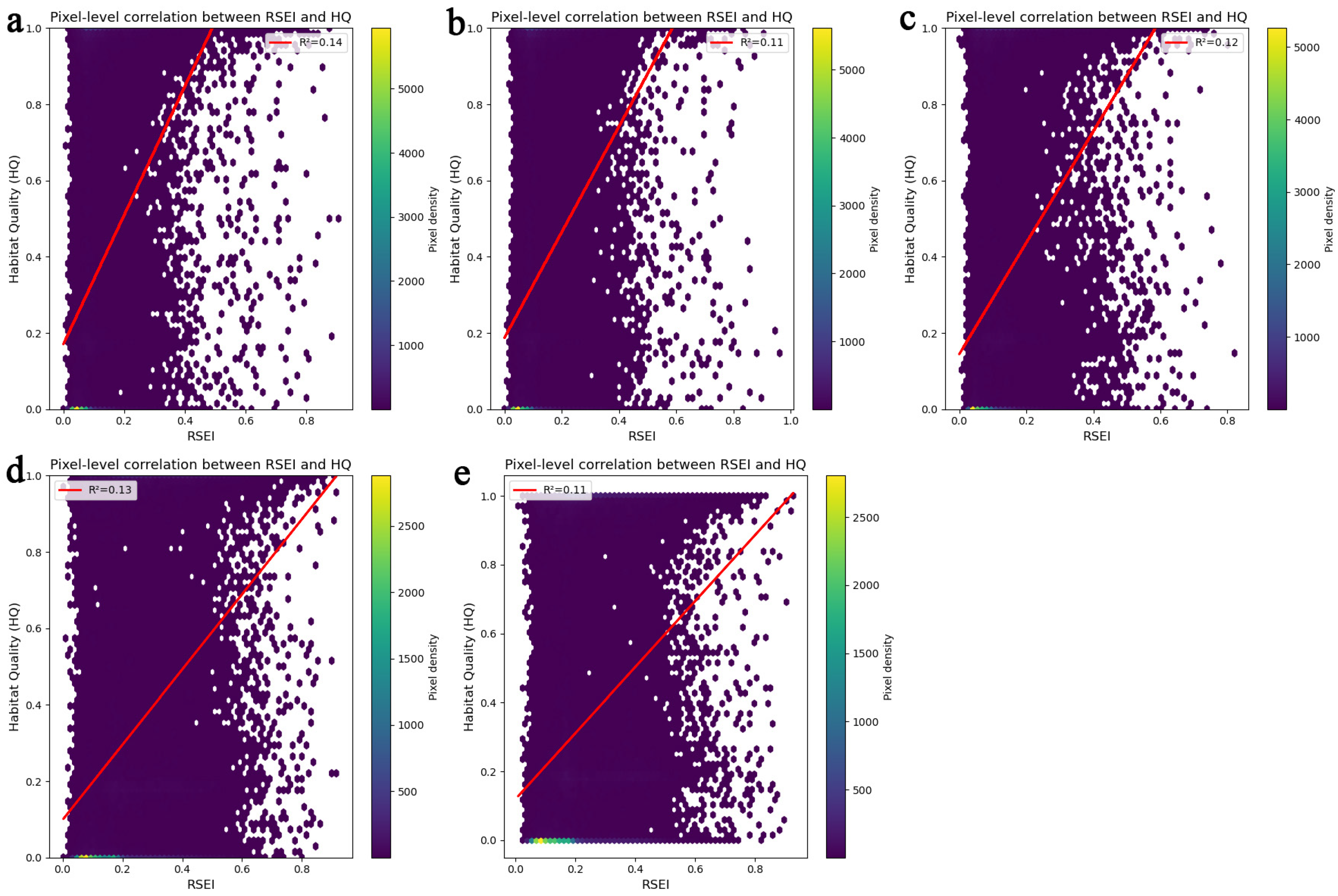
This study systematically examined the relationship between HQ and the RSEI in the UANSTM from 2000 to 2020 (Figure 6, Table 4). At the pixel scale, HQ exhibited a clear positive relationship with RSEI, indicating that regions with higher ecological quality tend to correspond to higher HQ. However, the coefficient of determination (R2 < 0.15) suggests that RSEI accounts for only approximately 15% of the spatial variation in HQ, and the scattered distribution of points implies a potential nonlinear or threshold-like relationship between the two indicators.
As shown in Table 4, HQ and RSEI were significantly positively correlated (Pearson r = 0.329, Spearman ρ = 0.446, p < 0.001) and exhibited strong spatial clustering (Moran’s I = 0.942 for HQ and 0.846 for RSEI, p = 0.001). This indicates that areas of high or low ecological and HQ are spatially contiguous rather than randomly distributed.

3.2.2. Characteristics of HQ Changes

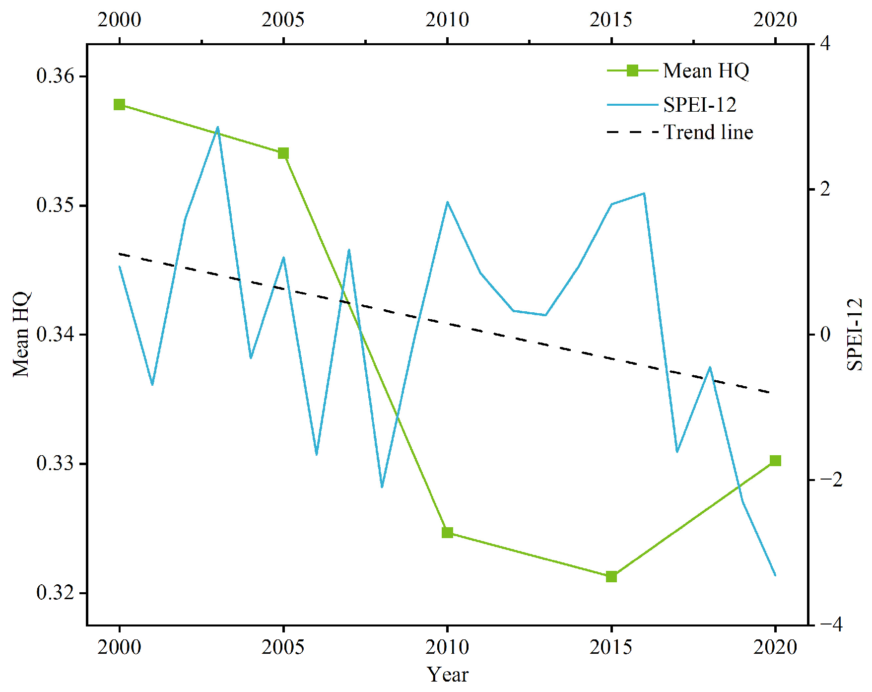
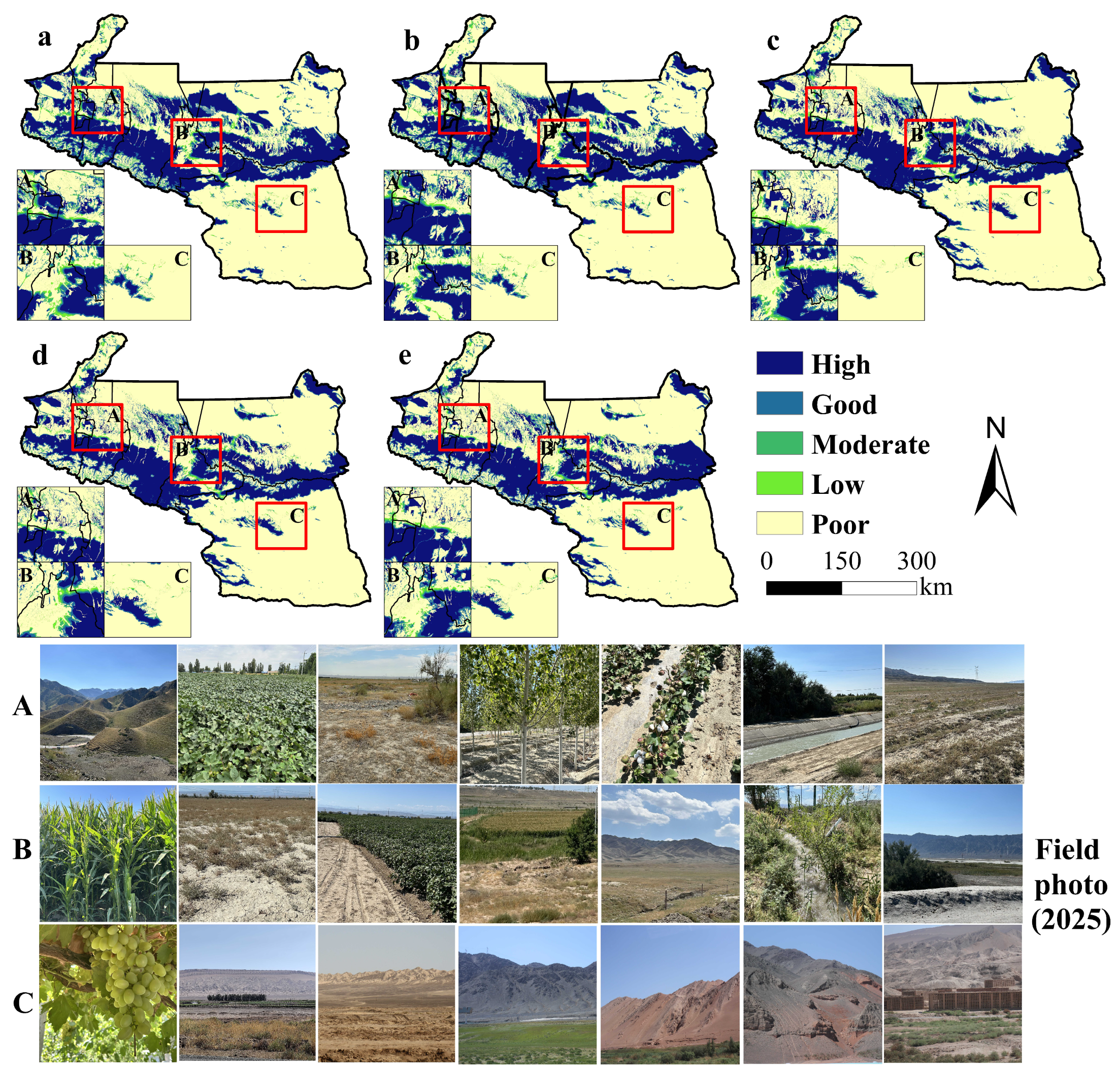
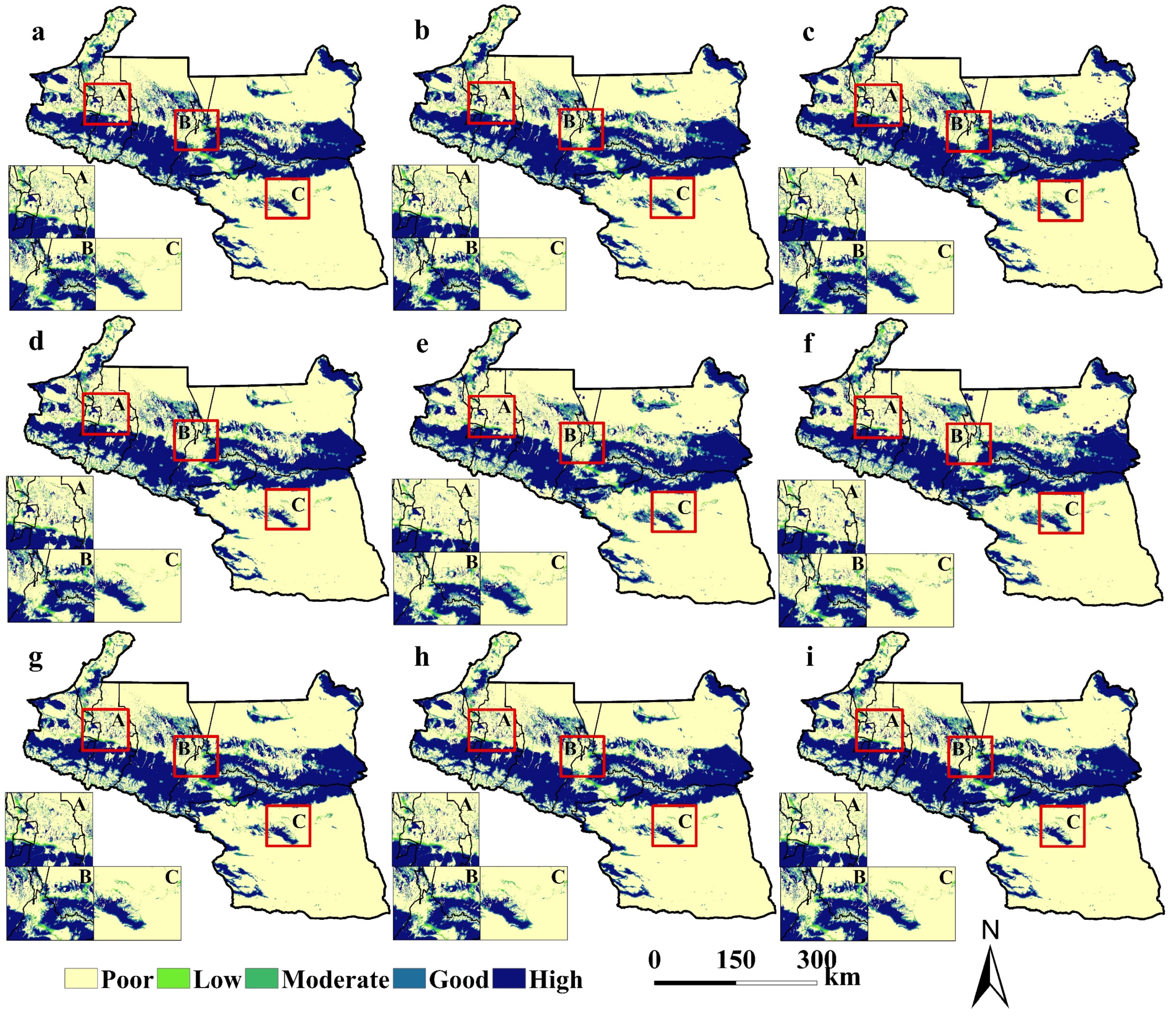
During the 2000–2020 period, the UANSTM exhibited a nonlinear trajectory of HQ dynamics (Figure 7), characterized by an initial decline followed by marginal recovery. Nevertheless, the overall HQ continued to decline, with the mean value dropping from 0.36 in 2000 to 0.33 in 2020. The most pronounced deterioration occurred between 2000 and 2010, with a statistically significant decline of 9.27% in HQ. HQ projections under divergent scenarios showed substantial divergence (Figure 8). Under SSP119, HQ is projected to increase steadily from 2020 to 2050, reaching 0.367 by 2050, representing an 11.21% increase, despite varying annualized change rates. Under SSP245, an initial 1.28% decline by 2030 is followed by recovery to 0.363 by 2050, corresponding to a 10.0% increase. SSP585 follows a similar pattern to SSP245, with a 0.04% decline by 2030 and a slower rebound to 0.349 by 2050, representing a 5.76% increase. Overall, HQ is expected to improve under all scenarios, albeit at varying rates. Spatially, the highest HQ is concentrated in the southern Changji Hui Autonomous Prefecture and the forest-grassland ecosystems of the Tianshan Mountain Nature Reserves, spanning counties such as Shawan, Usu, and Karamay. These regions owe their exceptional ecological integrity to rich species reservoirs, elevated biodiversity, and minimal anthropogenic disturbance. In contrast, degraded habitats predominantly characterize the Turpan Basin and northern Changji Prefecture, where intensive agricultural plains, urban settlements, and barren desert zones dominate the landscape patterns.
In the three representative sub-regions (A, B, and C), the HQ in regions A and B is markedly higher than in region C. Field investigations (Figure 7) conducted in August 2025 indicated that region A is primarily composed of grassland, cropland, and woodland. Most croplands rely on artificial irrigation, maintaining relatively high vegetation cover and ensuring good overall HQ, with only a few areas dominated by sparse grassland and Gobi land exhibiting relatively low levels. The land-use structure of region B is largely similar to that of region A, with only minor ecological differences; therefore, except for several localized Gobi areas, the overall HQ remains relatively high. By contrast, region C exhibits distinct geomorphological characteristics compared with regions A and B. It is dominated by extensive desert landscapes with only scattered oases, resulting in generally low vegetation cover and, consequently, significantly lower habitat quality than in regions A and B.
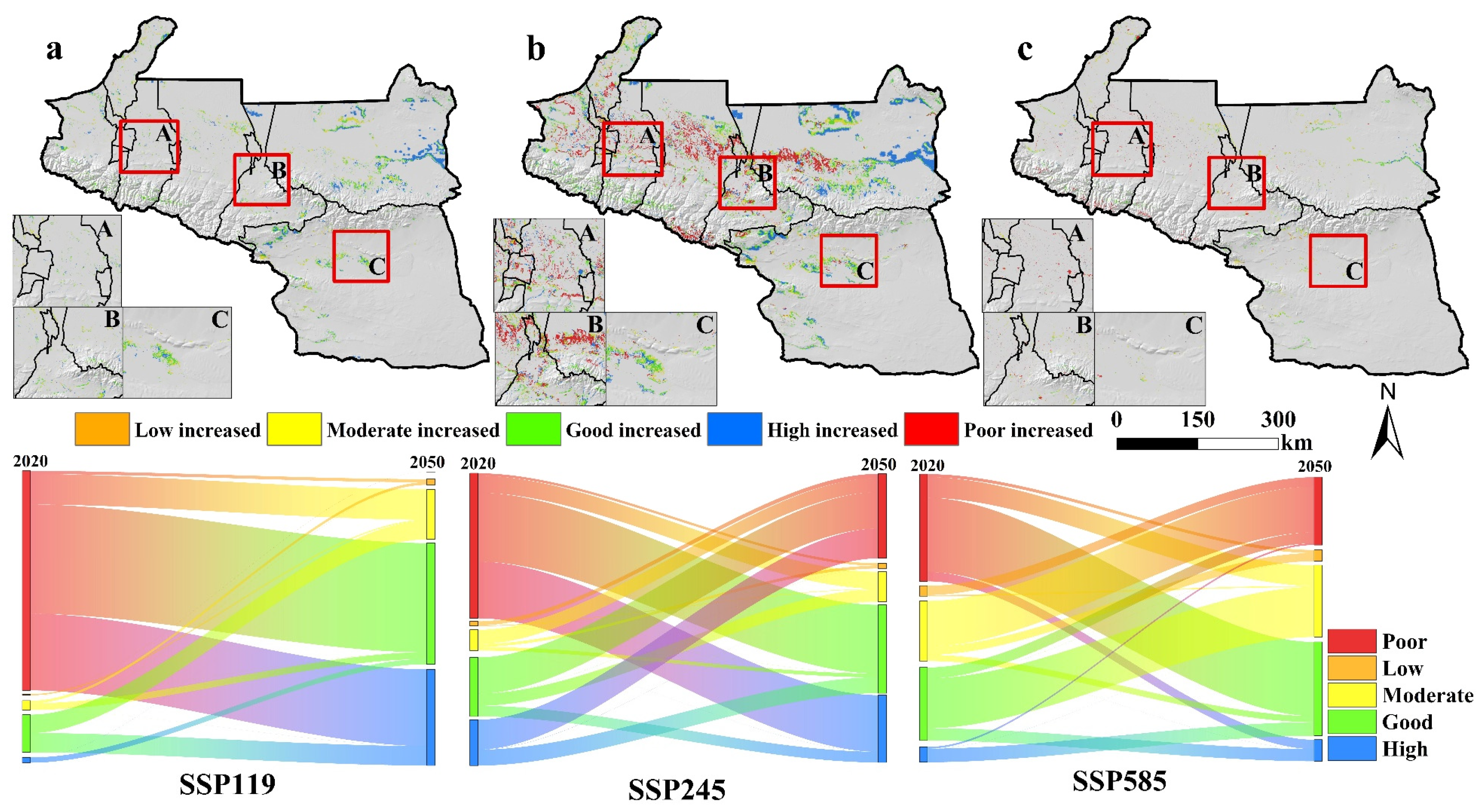
This study further examined the spatiotemporal transitions of HQ in the UANSTM under different scenarios during 2020–2050 (Figure 9, Table A11). The results indicated that under the SSP119 scenario, HQ exhibited an overall improving trend. The Sankey diagram revealed that Low-HQ areas were primarily converted to Moderate-HQ (755.96 km2), Good-HQ (2717.56 km2), and High-HQ (1909.11 km2), reflecting a continuous enhancement of ecosystem conditions. Spatially, these improvements were mainly concentrated in the Changji Hui Autonomous Prefecture and the northwestern part of Turpan. Under the SSP245 scenario, the transitions among HQ categories became more complex. Notably, Poor-HQ areas were largely converted to Good-HQ (5029.69 km2) and High-HQ (4139.35 km2), suggesting a substantial expansion of medium- and high-quality habitats. Spatially, HQ degradation was mainly observed in the central and northwestern regions of the study area, while the northeastern and partially southern regions exhibited gradual improvement. Under the SSP585 scenario, spatial transitions of HQ were relatively limited, although a numerical shift from Poor-HQ to Good-HQ (851.43 km2) and Moderate-HQ (237.18 km2) was still evident.
Overall, HQ in the study area is projected to improve gradually under all scenarios, primarily due to the continuous transformation of Poor-HQ into Moderate- and Good-HQ types. Spatially, HQ enhancement was predominantly distributed in the northeastern region—particularly in the Changji Hui Autonomous Prefecture—whereas degradation was concentrated in the oasis plains characterized by intensive human activities.

3.2.3. Spatiotemporal Uncertainty of Future HQ Predictions

Based on HQ raster datasets under multiple future scenarios, this study first calculated the cross-scenario mean and standard deviation for each pixel and derived the coefficient of variation (CV) as their ratio to quantify scenario-driven predictive uncertainty. A higher CV indicates greater discrepancies among scenarios and thus higher instability in predicted HQ, whereas a lower CV reflects more robust and consistent predictions.
The results show that the spatial distribution of CV in 2030, 2040, and 2050 exhibits temporal accumulation effects and regional heterogeneity (Figure 10). Temporally, CV values increase progressively over time, with high-uncertainty areas evolving from scattered patches in the near term to more contiguous clusters in the mid- to long-term periods, highlighting the cumulative amplification of scenario differences. Spatially, the mountain–plain transition zone, urban expansion frontiers, and the peripheries of oasis systems consistently exhibit high CV values. These areas are highly sensitive to land-use transitions and climatic gradients, making them hotspots of future prediction divergence. In contrast, land-cover types with relatively slow dynamics—such as forest, stable cropland, and grassland—generally show low CV values, indicating strong consistency across scenarios. Overall, areas with elevated uncertainty largely correspond to ecologically fragile zones or regions with intense land-use dynamics, underscoring the need to prioritize these areas in future ecological management and spatial planning.

3.3. Analysis of Habitat Quality Drivers

Spatial resolution emerged as a critical determinant modulating analytical outcomes in multiscale assessments. This study implemented six grids at different spatial scales to explore the spatial scale effect and identified the optimal scale for driver analysis based on the 80th percentile of q-values (Figure A3). The results indicated that the optimal scales for single-factor detection and interaction-factor detection differ. Based on these findings, we further investigated the driving factors of HQ changes at two distinct spatial scales.
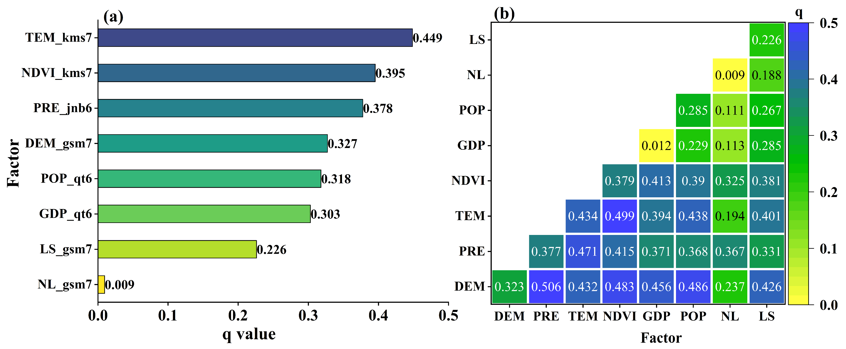
This study investigated the primary drivers of HQ changes in the UANSTM at a 3500 m spatial scale through single-factor analysis (Figure 11a). The results demonstrated that all driving factors exerted significant impacts on HQ (p < 0.01), with mean annual temperature exhibiting the strongest explanatory power (q = 0.449), primarily because temperature regulates ecosystem productivity and drought stress, thereby serving as the dominant climatic driver of the spatial heterogeneity in habitat quality. This was followed by NDVI (q = 0.395) and annual precipitation (q = 0.378), indicating that thermal-precipitation regime fluctuations and vegetation dynamics predominantly governed HQ variations. Among socioeconomic factors, population density (q = 0.318), GDP (q = 0.303), and livestock density (q = 0.226) emerged as particularly influential determinants, further substantiating the substantial anthropogenic pressures on ecosystem integrity.
This study further explored the interactive effects of these factors at a 1000 m spatial scale (Figure 11b). The results demonstrated that the interactions between natural factors exerted stronger effects on HQ, with the combination of DEM and annual precipitation showing particularly notable influence (q = 0.506). Interactions between socioeconomic factors and natural environmental factors also impacted HQ, such as those between population density and DEM (q = 0.486), and GDP and DEM (q = 0.456). Overall, the combined effects of natural-social factor interactions were consistently more influential on HQ than individual social factors alone.

4. Discussion

4.1. Drought Scenario Prediction

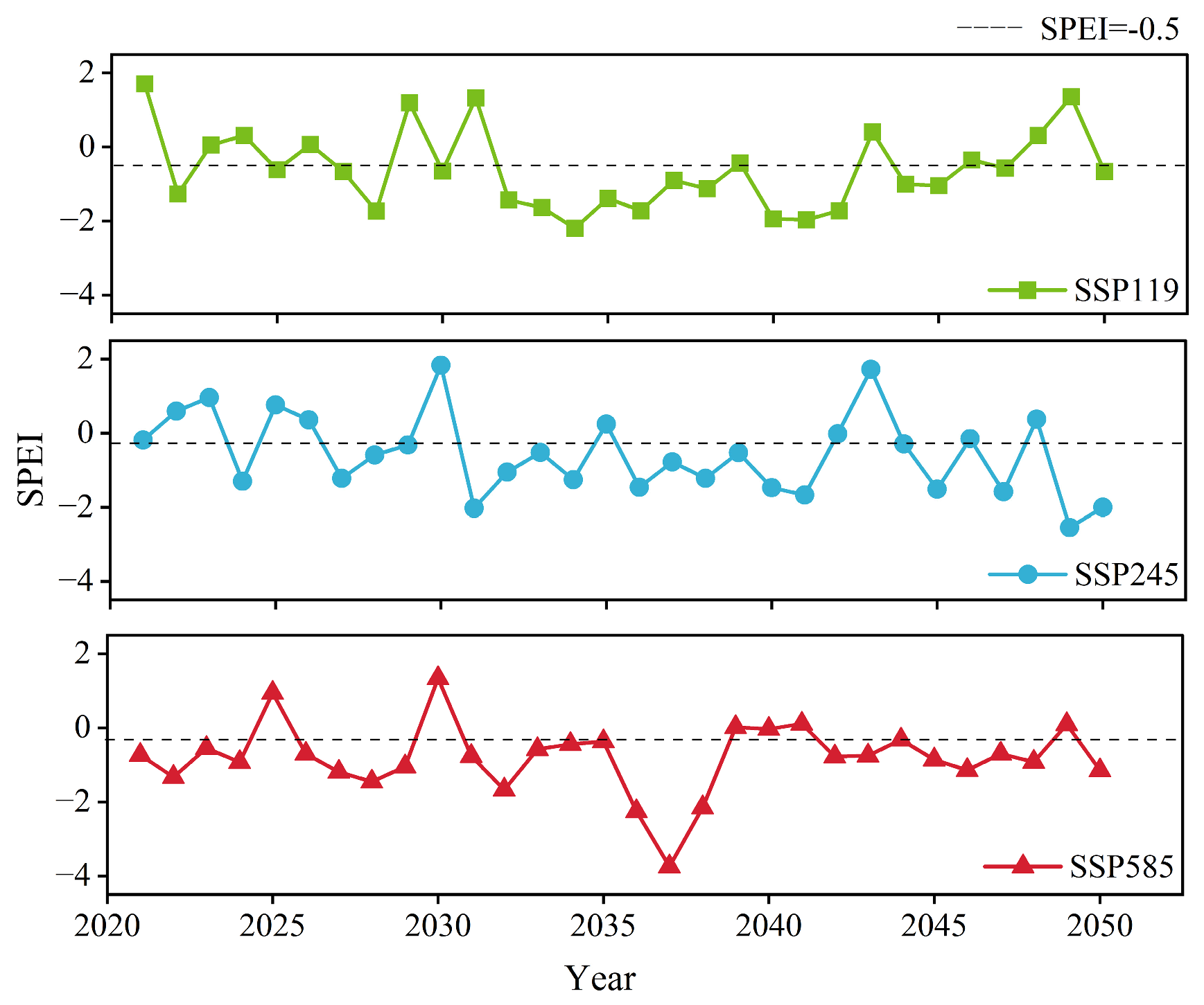
Based on CMIP6 climate data, this study quantified the 12-month SPEI under three scenarios (Figure A4). The December values of the 12-month SPEI from each year were selected as annual SPEI values to analyze drought variations across the UANSTM. Results demonstrated a fluctuating decline in SPEI values across all scenarios within the region. Under the SSP119 scenario, the UANSTM experienced 19 drought events, though with generally mild severity. The SSP245 scenario showed 17 drought events, including three extreme drought occurrences. In contrast, the high-emission SSP585 scenario exhibited the highest frequency of drought events, with persistent extreme drought conditions prevailing from 2036 to 2038. In summary, the UANSTM is projected to persist under arid climate conditions over the next three decades, a conclusion consistent with the findings of Shan et al. [37]. Additionally, studies by Su et al. and Ma et al. [27,38], which utilized CMIP6 data to predict future drought patterns in China, indicate a similarly significant intensification of drought in northwestern China. These projections closely align with the results of the present study.

4.2. The Corresponding Impact of Drought on Habitat Quality

HQ and SPEI-12 exhibited a generally positive correlation from 2000 to 2015 (Figure A5), suggesting that drought exerts a certain constraint on HQ. However, after 2015, drought intensity in the UANSTM increased significantly, yet HQ showed a slight recovery relative to previous levels. Moreover, simulation results further indicated that under different scenarios, HQ is expected to improve, whereas drought intensity will continue to intensify. Mechanistically, this pattern can be explained by both climate change and human activities. First, the “warm-wet” trend in northwestern China, characterized by rising temperatures and increased precipitation, has partially enhanced vegetation growth conditions, thereby promoting ecosystem function and HQ [55]. Second, the UANSTM is dominated by oasis agriculture. Consequently, even under intensified drought conditions, anthropogenic interventions—such as land reclamation, irrigation, and water infrastructure development—have partially decoupled the natural link between drought and vegetation water availability [56], further promoting positive trends in ecosystem quality. Collectively, these findings suggest that under future climate change, the influence of drought on HQ may gradually weaken.

4.3. Land Use Change Response to Habitat Quality

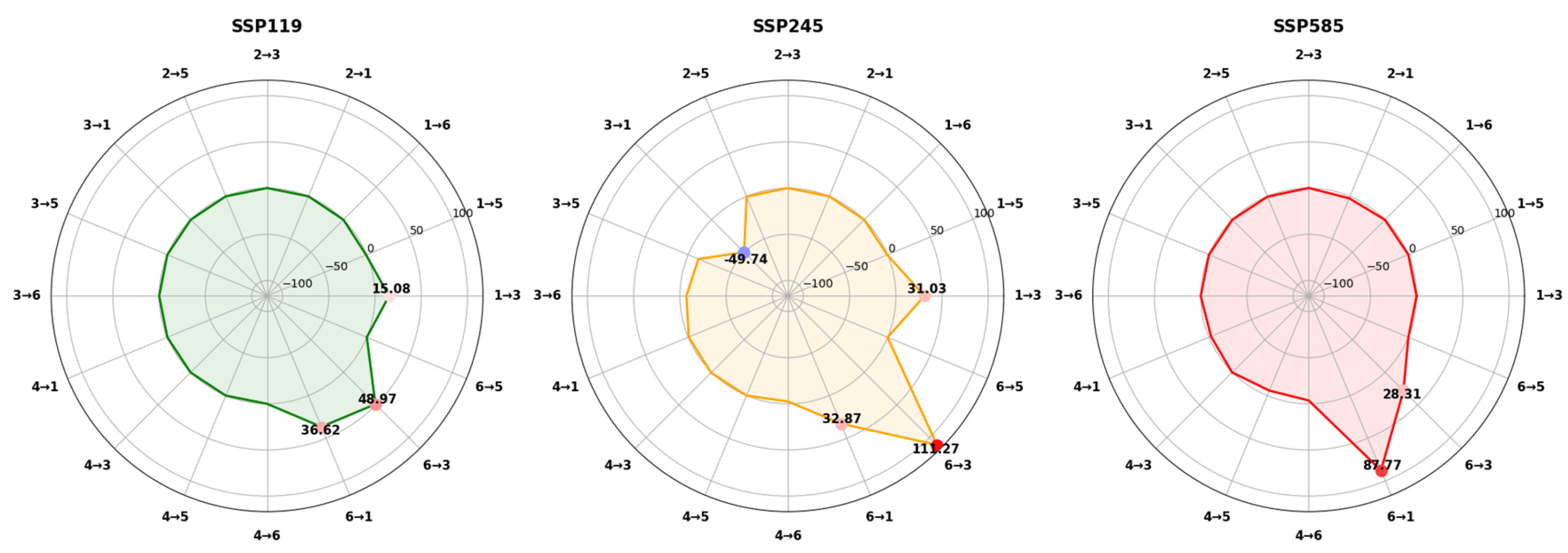
The distribution of HQ is closely linked to land use types. HQ in the UANSTM significantly declined from 2000 to 2010, primarily due to the implementation of the “Western Development Strategy”. During this period, regional economic expansion was prioritized, accompanied by intensive groundwater extraction, overgrazing, and large-scale land reclamation [57], which accelerated the degradation of forest and grassland with high habitat suitability, leading to a pronounced decline in HQ. Subsequently, the initiation of the “Three-North Shelterbelt Forest Program” and the enforcement of the “Grain for Green” policy effectively reversed this trend. These policies not only curtailed agricultural expansion and overexploitation but also promoted vegetation restoration through ecological compensation mechanisms and afforestation incentives [58]. Consequently, HQ experienced a slight improvement after 2010. Furthermore, under all three future scenarios, grassland with high habitat suitability exhibited sustained expansion, while unused land with low habitat suitability showed a substantial decline. This dual dynamic jointly enhanced regional HQ. To validate the above conclusion, this study further analyzed the contributions of land-use changes to habitat quality (HQ) under different climate scenarios from 2020 to 2050 (Figure A6). The results indicate that under the SSP119 scenario, the conversion of unused land to grassland and cropland was the primary driver of HQ improvement, with relative contributions of 48.97% and 36.62%, respectively. Under the SSP245 scenario, the conversion of unused land to grassland contributed substantially to HQ enhancement (111.27%), whereas the conversion of grassland to cropland had a negative contribution of 49.74%. Similarly, under the SSP585 scenario, the conversion of unused land to cropland and grassland also played a positive role in improving HQ.

4.4. Assessment of the Framework Established

This study established a multi-model coupling framework, incorporating drought scenarios based on previous research to assess the future evolutionary characteristics of HQ in the UANSTM. This approach enhances the scientific rigor and explanatory power of land use and HQ predictions in arid regions [30]. We further identified key drivers of HQ variation at optimal spatial scales, providing scientific guidance for rational land use planning and sustainable ecological development in arid and semi-arid regions [33]. However, this study has certain limitations. First, while the effects of drought on land use demand projections were considered, their influence on the spatial distribution of land use was not incorporated into the predictive model. Second, HQ changes are shaped not only by climatic factors but also by socioeconomic strategies, and different development policies may lead to varying HQ patterns [59,60]. Notably, explicit policy interventions, such as urban ecological redlines or expansion limits in highly sensitive areas, were not included. Incorporating such policy scenarios into the SD-PLUS model could further enhance its prescriptive value for sustainable land-use planning and ecological protection. Future research should integrate drought-induced spatial redistribution mechanisms along with relevant policy guidelines and natural hazard risks to comprehensively assess the interactions among land use, climate, and HQ in drought-prone regions.

5. Conclusions

In this study, the spatiotemporal evolution of land use, HQ under multiple future scenarios, and the driving mechanisms of HQ were quantified within the UANSTM using the integrated SD–PLUS–InVEST framework. The main conclusions are as follows: (i) Cultivated and construction land expanded markedly from 2000 to 2020, while forest and water areas continuously declined, and unused land—though fluctuating—remained the dominant land type. In the future (2020–2050), under all climate scenarios, cultivated land, grassland, and construction land are projected to continue expanding, with the proportion of unused land decreasing by approximately 9.8%; among these, the SSP585 scenario exhibits the most pronounced expansion trend. (ii) Between 2000 and 2020, HQ declined from 0.36 to 0.33, primarily due to intensive agriculture, urbanization, and was significantly positively correlated with the RSEI; (Pearson r = 0.329, Spearman ρ = 0.446, p < 0.001). From 2020 to 2050, HQ is projected to improve under all climate scenarios, mainly through the conversion of low-quality areas into moderate- and high-quality habitats, with the greatest improvement under SSP119 and the least under SSP585. (iii) HQ was mainly driven by climatic and vegetation factors, with interactions between natural factors and between natural and socioeconomic factors were more influential than single factors, emphasizing the dominant role of coupled natural–social drivers in shaping HQ patterns. Although the current framework provides robust projections, the uncertainty associated with future HQ simulations—particularly those arising from the parameterization of land-demand and drought-intensity models—remains to be quantified in subsequent work. Nonetheless, the proposed integrative approach demonstrates strong potential for application in other arid and semi-arid regions, offering methodological guidance for biodiversity conservation and climate-resilient land-use planning.

Author Contributions

Conceptualization, R.J. and L.H.; methodology, R.J. and L.H.; software, R.J.; validation, R.J., Z.H. and Y.Z.; formal analysis, R.J.; investigation, R.J., Z.L. and D.L.; resources, R.J. and Y.H.; data curation, R.J.; writing—original draft preparation, R.J. and L.H.; writing—review and editing, R.J., Z.H., Y.Z., F.L. and Z.L.; visualization, R.J.; supervision, Z.H.; funding acquisition, L.H. All authors have read and agreed to the published version of the manuscript.

Funding

This research was supported by the Key Research and Development Program of the Ministry of Science and Technology (The Third Comprehensive Scientific Expedition to Xinjiang) (2023xjkk0103); the National Natural Science Foundation of China (Grant No. 42301456); the Natural Science Foundation of Sichuan Province (Grant No. 2025ZNSFSC0321).

Data Availability Statement

The datasets generated and/or analyzed during the current study are available from the corresponding author upon reasonable request.

Acknowledgments

The author appreciates all the data provided by each open database. The author thanks anonymous reviewers and academic editors for their comments.

Conflicts of Interest

The authors declare no conflicts of interest.

Appendix A

Appendix A.1

Table A1. SPEI Classification Levels.
SPEICategories
SPEI > −0.5Near normal
−1.0 < SPEI ≤ −0.5Slight dry
−1.5 < SPEI ≤ −1.0Moderately dry
−2.0 < SPEI ≤ −1.5Severely dry
SPEI ≥ −2.0Extremely dry
Table A2. Parameter settings under different climates from 2020 to 2050.
Parameter Type2020–20302030–20402040–2050
SSP119SSP245SSP585SSP119SSP245SSP585SSP119SSP245SSP585
AGR3.78%3.53%3.85%2.94%3.27%3.73%2.63%3.08%3.31%
APR0.53‰0.74‰0.61‰0.44‰0.66‰0.52‰0.26‰0.59‰0.35‰
APV (mm)2.55 −0.32 7.82 −4.29 2.17 −3.93 3.80 −0.94 −1.80
ATV (°C)0.08 0.08 0.09 0.05 −0.01 0.09 −0.02 0.18 −0.03
Table A3. Main equations of SD model.
Main EquationsUnit
Population = INTEG (Population change, 530.761)ten thousand
Population change = Population × Population change rateten thousand
Primary industry investment = 147,072 + 0.041 × Fixed investmentten thousand
Secondary and tertiary industry investment = −147,072 + 0.958933 × Fixed investmentten thousand
Urban population = −185.636 + 1.0238 × Populationten thousand
Rural population = Population − Urban populationten thousand
Urban construction land demand = −450.225 + 2.02 × Urban populationkm2
Rural construction land demand = EXP (5.9876 − 124.842/Rural population)km2
Agricultural investment = 266,071 + 0.146765 × Primary industry investmentten thousand
Fishery investment = −9818.04 + 0.01556 × Primary industry investmentten thousand
Forestry investment = 17,333.4 + 0.018881 × Primary industry investmentten thousand
Livestock investment = −100,921 + 0.274569 × Primary industry investmentten thousand
Construction land change = −621.716 + 3.12953 × Rural construction land demand + 2.26594 × Urban construction land demand + 0.00013 × Secondary and tertiary industry investmentkm2
Grassland change = 4741.63 + 0.000346 × Livestock investment + 9.27408 × Construction land change − 0.2622 × Livestock product demand − 241.191 × Average annual temperature + 5.02998 × Annual precipitation − 71.4336 × SPEIkm2
Forest change = −44.2848 − 2.5 × 10⁻⁵ × Forestry investment − 83.145 × Area of farmland returned to forest + 1.32188 × Average annual temperature + 0.5896 × Annual precipitation − 11.7385 × SPEIkm2
Water change = 392.3513 + 0.00768 × Fishery investment − 0.13233 × Aquatic product demand − 69.08913 × Average annual temperature + 1.96969 × Annual precipitation + 0.69345 × SPEIkm2
Cultivated land change = 725.398 − 0.01212 × Food demand + 366.8 × Area of farmland returned to forest + 0.001607 × Agricultural investment − 9.43386 × Construction land change − 67.8428 × Average annual temperature + 3.39966 × Annual precipitation − 58.0908 × SPEIkm2
Unused land change = −(Construction land change + Grassland change + Forest change + Water change + Cultivated land change)km2
Table A4. Land-Use Simulation Accuracy Verification.
Land Use TypesActual Value in 2020Predicted Value in 2020Relative Error
(km2)(km2)(%)
Cultivated Land22,063.7222,067.30.016
Forest3047.43045.55−0.061
Grassland58,798.6258,795.8−0.005
Water2025.042023.46−0.078
Construction Land3644.753646.940.060
Unused Land104,408.69104,405−0.004
Table A5. SD model sensitivity analysis results.
ParameterReduced by 10%Increase by 10%
Population change rate0.0120.002
GDP change rate0.0190.019
Primary industry investment0.0600.060
Secondary and tertiary industry investment−0.004−0.004
Urban construction land demand−0.283−0.281
Rural construction land demand−0.189−0.176
Agricultural investment0.1640.164
Fishery investment0.0320.032
Forestry investment0.1290.129
Livestock investment0.0300.030
Table A6. Land Transfer Matrix under Different Scenarios and Weights of Each Land-Use Type.
Cultivated LandForestGrasslandWaterConstruction LandUnused Land
Cultivated Land111110110110111011
Forest001111111111011001
Grassland011111111111011011
Water001101111111001011
Construction Land000100100000111000
Unused Land111111111111111111
Weight of neighborhood0.37050.0282100.24060.2308
Note: Green for SSP119, blue for SSP245, red for SSP585. When the corresponding value of the matrix is set to 0, it shows that the two cannot be converted to each other; otherwise, it is set to 1.
Table A7. HQ robustness test.
Parameter VariationPearson’s rRMSEStability Level
Threat weight + 10%10High
Threat weight − 10%10High
Decay distance + 10%0.9999640.004528High
Decay distance − 10%0.9999610.004723High
Table A8. Linear Regression Trend Significance Test for Each Land-Use Type.
Land UseSlopeR2p
Cultivated Land386.470.8740.0197
Forest−143.540.7860.0452
Grassland−211.370.5850.1319
Water−97.20.770.0505
Construction Land89.550.980.0012
Unused Land−23.130.0190.8241
Table A9. Model performance metrics (FoM and Kappa) for 2010–2015 and 2010–2020 backcasts.
Start_YearEnd_YearFoMKappa
201020200.97610.8991
201020150.99330.9849
Table A10. Land Use Demands for Each Land Type under Different Scenarios (km2).
Land Use TypesSSP119SSP245SSP585
203020402050203020402050203020402050
Cultivated Land21,219.825,051.334,709.121,812.625,863.034,733.222,475.528,290.439,762.7
Forest2721.62495.72216.02728.12464.02057.92631.92339.02008.6
Grassland60,167.062,105.065,347.759,483.261,768.865,085.559,493.360,022.761,048.1
Water1394.31336.51285.31218.71151.71181.11272.01042.41000.9
Construction Land4620.55423.35970.04679.55497.06019.34818.45678.46190.5
Unused Land103,08296,984.184,541.4104,49898,068.984,751.1102,40593,733.979,063.6
Table A11. Area of Habitat Quality Changes from 2020 to 2050 under Different Scenarios (km2).
SSP119 PoorLowModerateGoodHigh
Poor124,695.178.57755.962717.561909.11
Low0.111238.9130.980.020
Moderate065.744439.68166.661.23
Good00.07456.6114,384.95483.03
High000.37131.7714,384.95
SSP245 PoorLowModerateGoodHigh
Poor119,560.9181.931244.435029.694139.35
Low304.24916.5948.680.510
Moderate1041.77203.993151.48273.312.76
Good2651.152.9888.810,997.49784.32
High2177.89015.551164.8539,243.99
SSP585 PoorLowModerateGoodHigh
Poor128,924.635.37237.18851.43107.69
Low108.051148.2813.6900
Moderate525.3394.913982.1570.820.1
Good125.730.17573.9114,484.11140.74
High20.0900.57157.3542,424.27

Appendix A.2

Figure A1. Spatial disagreement maps between simulated and actual land-use patterns for the 2015 and 2020 periods.
Agronomy 15 02704 g0a1
Figure A2. Predicted Land Use Demand for Each Land Type.
Agronomy 15 02704 g0a2
Figure A3. Optimal scale detection results from the OMGD, (a): Single-Factor Detection; (b): Factor Interaction Detection.
Agronomy 15 02704 g0a3
Figure A4. SPEI Changes under Different Scenarios from 2020 to 2050.
Agronomy 15 02704 g0a4
Figure A5. Trends of SPEI-12 and HQ changes from 2000 to 2020.
Agronomy 15 02704 g0a5
Figure A6. Contribution of Land-Use Changes to Habitat Quality under Different Scenarios. Note: Numbers represent land-use types: 1 = Cultivated Land, 2 = Forest, 3 = Grassland, 4 = Water, 5 = Construction Land, 6 = Unused Land; “X→Y” indicates a transition from type X to type Y.
Agronomy 15 02704 g0a6
Figure A7. Spatial Distribution of RSEI from 2000 to 2020. (a) 2000, (b) 2005, (c) 2010, (d) 2015, (e) 2020. A, B, and C indicate the zoomed areas selected for detailed analysis.
Agronomy 15 02704 g0a7

Appendix B. Field Quadrat Validation

To ensure the reliability of the calculated HQ values, this study conducted a field-based qualitative validation using 1 m × 1 m vegetation quadrats, each further subdivided into 10 × 10 sub-grids. The vegetation coverage within each quadrat was visually assessed (Figure A8) to qualitatively evaluate the local habitat condition. A total of nine sampling sites were selected for comparison (Table A12). The results demonstrated a strong overall consistency between the simulated HQ values and the observed vegetation coverage, confirming the validity of the HQ estimation.
Table A12. Actual Vegetation Coverage and the Corresponding HQ Values.
SampleHQ ValueVegetation Coverage
a0.1838%
b0.83665%
c0.90899%
d0.2009%
e0.59342%
f04%
g0.78480%
h0.60965%
i0.45316%
Figure A8. Field investigation. (a-i) sampes.
Agronomy 15 02704 g0a8

References

  1. Wu, Y.; Wang, J.; Gou, A. Research on the Evolution Characteristics, Driving Mechanisms and Multi-Scenario Simulation of Habitat Quality in the Guangdong-Hong Kong-Macao Greater Bay Based on Multi-Model Coupling. Sci. Total Environ. 2024, 924, 171263. [Google Scholar] [CrossRef]
  2. Qin, X.; Yang, Q.; Wang, L. The Evolution of Habitat Quality and Its Response to Land Use Change in the Coastal China, 1985–2020. Sci. Total Environ. 2024, 952, 175930. [Google Scholar] [CrossRef]
  3. Bai, L.; Xiu, C.; Feng, X.; Liu, D. Influence of Urbanization on Regional Habitat Quality:A Case Study of Changchun City. Habitat Int. 2019, 93, 102042. [Google Scholar] [CrossRef]
  4. Huang, J.; Tang, Z.; Liu, D.; He, J. Ecological Response to Urban Development in a Changing Socio-Economic and Climate Context: Policy Implications for Balancing Regional Development and Habitat Conservation. Land Use Policy 2020, 97, 104772. [Google Scholar] [CrossRef]
  5. Wu, Y.; Zhang, X.; Li, C.; Xu, Y.; Hao, F.; Yin, G. Ecosystem Service Trade-Offs and Synergies under Influence of Climate and Land Cover Change in an Afforested Semiarid Basin, China. Ecol. Eng. 2021, 159, 106083. [Google Scholar] [CrossRef]
  6. Fulford, R.S.; Russell, M.; Myers, M.; Malish, M.; Delmaine, A. Models Help Set Ecosystem Service Baselines for Restoration Assessment. J. Environ. Manag. 2022, 317, 115411. [Google Scholar] [CrossRef]
  7. Li, Y.; Liu, W.; Feng, Q.; Zhu, M.; Yang, L.; Zhang, J.; Yin, X. The Role of Land Use Change in Affecting Ecosystem Services and the Ecological Security Pattern of the Hexi Regions, Northwest China. Sci. Total Environ. 2023, 855, 158940. [Google Scholar] [CrossRef]
  8. Li, S.; Hong, Z.; Xue, X.; Zheng, X.; Du, S.; Liu, X. Evolution Characteristics and Multi-Scenario Prediction of Habitat Quality in Yulin City Based on PLUS and InVEST Models. Sci. Rep. 2024, 14, 11852. [Google Scholar] [CrossRef]
  9. Desta, H. Local Perceptions of Ecosystem Services and Human-Induced Degradation of Lake Ziway in the Rift Valley Region of Ethiopia. Ecol. Indic. 2021, 127, 107786. [Google Scholar] [CrossRef]
  10. Wang, S.; Li, R.; Wu, Y.; Zhao, S. Effects of Multi-Temporal Scale Drought on Vegetation Dynamics in Inner Mongolia from 1982 to 2015, China. Ecol. Indic. 2022, 136, 108666. [Google Scholar] [CrossRef]
  11. Zabel, F.; Putzenlechner, B.; Mauser, W. Global Agricultural Land Resources—A High Resolution Suitability Evaluation and Its Perspectives until 2100 under Climate Change Conditions. PLoS ONE 2014, 9, e107522. [Google Scholar] [CrossRef]
  12. Guise, I.; Silva, B.; Mestre, F.; Muñoz-Rojas, J.; Duarte, M.F.; Herrera, J.M. Climate Change Is Expected to Severely Impact Protected Designation of Origin Olive Growing Regions over the Iberian Peninsula. Agric. Syst. 2024, 220, 104108. [Google Scholar] [CrossRef]
  13. Chen, W.; Wang, G.; Gu, T.; Fang, C.; Pan, S.; Zeng, J.; Wu, J. Simulating the Impact of Urban Expansion on Ecosystem Services in Chinese Urban Agglomerations: A Multi-Scenario Perspective. Environ. Impact Assess. Rev. 2023, 103, 107275. [Google Scholar] [CrossRef]
  14. Zeng, W.; He, Z.; Bai, W.; He, L.; Chen, X.; Chen, J. Identification of Ecological Security Patterns of Alpine Wetland Grasslands Based on Landscape Ecological Risks: A Study in Zoigê County. Sci. Total Environ. 2024, 928, 172302. [Google Scholar] [CrossRef]
  15. Ashrafi, S.; Kerachian, R.; Pourmoghim, P.; Behboudian, M.; Motlaghzadeh, K. Evaluating and Improving the Sustainability of Ecosystem Services in River Basins under Climate Change. Sci. Total Environ. 2022, 806, 150702. [Google Scholar] [CrossRef]
  16. Polasky, S.; Nelson, E.; Pennington, D.; Johnson, K.A. The Impact of Land-Use Change on Ecosystem Services, Biodiversity and Returns to Landowners: A Case Study in the State of Minnesota. Environ. Resour. Econ. 2011, 48, 219–242. [Google Scholar] [CrossRef]
  17. Hu, F.; Zhang, Y.; Guo, Y.; Zhang, P.; Lv, S.; Zhang, C. Spatial and temporal changes in land use and habitat quality in the Weihe River Basin based on the PLUS and InVEST models and predictions. Arid. Land Geogr. 2022, 45, 1125–1136. [Google Scholar]
  18. Tian, C.; Zhong, J.; You, Q.; Fang, C.; Hu, Q.; Liang, J.; He, J.; Yang, W. Land Use Modeling and Habitat Quality Assessment under Climate Scenarios: A Case Study of the Poyang Lake Basin. Ecol. Indic. 2025, 172, 113292. [Google Scholar] [CrossRef]
  19. Luo, Y.; Fang, S.; Wu, H.; Zhou, X.; He, Z.; Gao, L. Spatial and Temporal Evolution of Habitat Quality and Its Shrinkage Effect in Shrinking Cities: Evidence from Northeast China. Ecol. Indic. 2024, 161, 111919. [Google Scholar] [CrossRef]
  20. Cai, X.; Li, Z.; Liang, Y. Tempo-Spatial Changes of Ecological Vulnerability in the Arid Area Based on Ordered Weighted Average Model. Ecol. Indic. 2021, 133, 108398. [Google Scholar] [CrossRef]
  21. Zhang, L.; Fang, C.; Zhu, C.; Gao, Q. Ecosystem Service Trade-Offs and Identification of Eco-Optimal Regions in Urban Agglomerations in Arid Regions of China. J. Clean. Prod. 2022, 373, 133823. [Google Scholar] [CrossRef]
  22. Ge, Y.; Li, C.; Zhang, T.; Wang, B. Temporal and Spatial Change of Habitat Quality and Its Driving Forces: The Case of Tacheng Region, China. Front. Environ. Sci. 2023, 11, 1118179. [Google Scholar] [CrossRef]
  23. Wei, Q.; Abudureheman, M.; Halike, A.; Yao, K.; Yao, L.; Tang, H.; Tuheti, B. Temporal and Spatial Variation Analysis of Habitat Quality on the PLUS-InVEST Model for Ebinur Lake Basin, China. Ecol. Indic. 2022, 145, 109632. [Google Scholar] [CrossRef]
  24. Chen, Q.; Ning, Y. Projecting LUCC Dynamics and Ecosystem Services in an Emerging Urban Agglomeration under SSP-RCP Scenarios and Their Management Implications. Sci. Total Environ. 2024, 949, 175100. [Google Scholar] [CrossRef]
  25. Wu, J.; Luo, J.; Zhang, H.; Qin, S.; Yu, M. Projections of Land Use Change and Habitat Quality Assessment by Coupling Climate Change and Development Patterns. Sci. Total Environ. 2022, 847, 157491. [Google Scholar] [CrossRef]
  26. Wei, R.; Fan, Y.; Wu, H.; Zheng, K.; Fan, J.; Liu, Z.; Xuan, J.; Zhou, J. The Value of Ecosystem Services in Arid and Semi-Arid Regions: A Multi-Scenario Analysis of Land Use Simulation in the Kashgar Region of Xinjiang. Ecol. Model. 2024, 488, 110579. [Google Scholar] [CrossRef]
  27. Su, B.; Huang, J.; Mondal, S.K.; Zhai, J.; Wang, Y.; Wen, S.; Gao, M.; Lv, Y.; Jiang, S.; Jiang, T.; et al. Insight from CMIP6 SSP-RCP Scenarios for Future Drought Characteristics in China. Atmos. Res. 2021, 250, 105375. [Google Scholar] [CrossRef]
  28. Mathbout, S.; Martin-Vide, J.; Bustins, J.A.L. Drought Characteristics Projections Based on CMIP6 Climate Change Scenarios in Syria. J. Hydrol. Reg. Stud. 2023, 50, 101581. [Google Scholar] [CrossRef]
  29. Li, Q.; Wang, C.; Feng, T.; Du, C.; Zhang, B. Multi-Scenario Prediction of Land Use Change and Carbon Storage in Shaanxi Province Based on the SD-PLUS Coupled Model. Chin. J. Soil Water Conserv. 2024, 38, 195–206+215. [Google Scholar] [CrossRef]
  30. Huang, H.; Xue, J.; Feng, X.; Zhao, J.; Sun, H.; Hu, Y.; Ma, Y. Thriving Arid Oasis Urban Agglomerations: Optimizing Ecosystem Services Pattern under Future Climate Change Scenarios Using Dynamic Bayesian Network. J. Environ. Manag. 2024, 350, 119612. [Google Scholar] [CrossRef]
  31. Sui, L.; Yan, Z.; Li, K.; He, P.; Ma, Y.; Zhang, R. Prediction of habitat quality in the Ili River Valley under the influence of human activities and climate change. Arid. Land Geogr. 2024, 47, 104–116. [Google Scholar]
  32. Ji, X.; Sun, Y.; Guo, W.; Zhao, C.; Li, K. Land Use and Habitat Quality Change in the Yellow River Basin: A Perspective with Different CMIP6-Based Scenarios and Multiple Scales. J. Environ. Manag. 2023, 345, 118729. [Google Scholar] [CrossRef] [PubMed]
  33. Yue, Z.; Xiao, C.; Feng, Z.; Wang, Y.; Yan, H. Accelerating Decline of Habitat Quality in Chinese Border Areas. Resour. Conserv. Recycl. 2024, 206, 107665. [Google Scholar] [CrossRef]
  34. Guo, Y.; Wu, Z.; Zheng, Z.; Li, X. An Optimal Multivariate-Stratification Geographical Detector Model for Revealing the Impact of Multi-Factor Combinations on the Dependent Variable. GIScience Remote Sens. 2024, 61, 2422941. [Google Scholar] [CrossRef]
  35. Peng, S.; Ding, Y.; Wen, Z.; Chen, Y.; Cao, Y.; Ren, J. Spatiotemporal Change and Trend Analysis of Potential Evapotranspiration over the Loess Plateau of China during 2011–2100. Agric. For. Meteorol. 2017, 233, 183–194. [Google Scholar] [CrossRef]
  36. Jiang, T.; Su, B.; Wang, Y.; Wang, G.; Luo, Y.; Zhai, J.; Huang, J.; Jing, C.; Gao, M.; Lin, Q.; et al. Gridded datasets for population and economy under Shared Socioeconomic Pathways for 2020–2100. Adv. Clim. Change Res. 2022, 18, 381–383. [Google Scholar]
  37. Shan, J.; Zhu, R.; Yin, Z.; Yang, H.; Zhang, W.; Fang, C. Spatial and temporal variation of drought in Northwest China based on CMIP6 model. Arid Zone Res. 2024, 41, 717–729. [Google Scholar] [CrossRef]
  38. Ma, Z.; Sun, P.; Zhang, Q.; Zou, Y.; Lv, Y.; Li, H.; Chen, D. The Characteristics and Evaluation of Future Droughts across China through the CMIP6 Multi-Model Ensemble. Remote Sens. 2022, 14, 1097. [Google Scholar] [CrossRef]
  39. Tao, H.; Borth, H.; Fraedrich, K.; Su, B.; Zhu, X. Drought and Wetness Variability in the Tarim River Basin and Connection to Large-Scale Atmospheric Circulation. Int. J. Climatol. 2014, 34, 2678–2684. [Google Scholar] [CrossRef]
  40. Gómez, F.; Lagos, O.; Gil, P.M.; Jara, J.; Zaccaria, D. Assessment of Reference Evapotranspiration Forecasting in the Mediterranean Climate of Central Chile Using the ASCE Standardized Penman-Monteith Equation, the Hargreaves-Samani Equation, and Weather Predictions from the Global Forecast System Model. Sci. Total Environ. 2024, 957, 177606. [Google Scholar] [CrossRef]
  41. Hargreaves, G.H.; Allen, R.G. History and Evaluation of Hargreaves Evapotranspiration Equation. J. Irrig. Drain. Eng. 2003, 129, 53–63. [Google Scholar] [CrossRef]
  42. Zhang, Z.; Li, X.; Liu, X.; Zhao, K. Dynamic Simulation and Projection of Land Use Change Using System Dynamics Model in the Chinese Tianshan Mountainous Region, Central Asia. Ecol. Model. 2024, 487, 110564. [Google Scholar] [CrossRef]
  43. Huang, J.; Qin, D.; Jiang, T.; Wang, Y.; Feng, Z.; Zhai, J.; Cao, L.; Chao, Q.; Xu, X.; Wang, G.; et al. Effect of Fertility Policy Changes on the Population Structure and Economy of China: From the Perspective of the Shared Socioeconomic Pathways. Earth’s Future 2019, 7, 250–265. [Google Scholar] [CrossRef]
  44. Zhang, S.; Yang, P.; Xia, J.; Wang, W.; Cai, W.; Chen, N.; Hu, S.; Luo, X.; Li, J.; Zhan, C. Land Use/Land Cover Prediction and Analysis of the Middle Reaches of the Yangtze River under Different Scenarios. Sci. Total Environ. 2022, 833, 155238. [Google Scholar] [CrossRef] [PubMed]
  45. Zhang, P.; Liu, L.; Yang, L.; Zhao, J.; Li, Y.; Qi, Y.; Ma, X.; Cao, L. Exploring the Response of Ecosystem Service Value to Land Use Changes under Multiple Scenarios Coupling a Mixed-Cell Cellular Automata Model and System Dynamics Model in Xi’an, China. Ecol. Indic. 2023, 147, 110009. [Google Scholar] [CrossRef]
  46. Gu, M.; Ye, C.; Li, X.; Hu, M. Scenario Simulation of Land Use Change in Jiangxi Province Based on SD Model. Geogr. Geo-Inf. Sci. 2022, 38, 95–103. [Google Scholar]
  47. Liang, X.; Guan, Q.; Clarke, K.C.; Liu, S.; Wang, B.; Yao, Y. Understanding the Drivers of Sustainable Land Expansion Using a Patch-Generating Land Use Simulation (PLUS) Model: A Case Study in Wuhan, China. Comput. Environ. Urban Syst. 2021, 85, 101569. [Google Scholar] [CrossRef]
  48. Luan, C.; Liu, R.; Li, Y.; Zhang, Q. Comparison of Various Models for Multi-Scenario Simulation of Land Use/Land Cover to Predict Ecosystem Service Value: A Case Study of Harbin-Changchun Urban Agglomeration, China. J. Clean. Prod. 2024, 478, 144012. [Google Scholar] [CrossRef]
  49. Fu, Y.; Lu, X.; Zhao, Y.; Zeng, X.; Xia, L. Assessment Impacts of Weather and Land Use/Land Cover (LULC) Change on Urban Vegetation Net Primary Productivity (NPP): A Case Study in Guangzhou, China. Remote Sens. 2013, 5, 4125–4144. [Google Scholar] [CrossRef]
  50. Wang, B.; Liao, J.; Zhu, W.; Qiu, Q.; Wang, L.; Tang, L. The weight of neighborhood setting of the FLUS model based on a historical scenario: A case study of land use simulation of urban agglomeration of the Golden Triangle of Southern Fujian in 2030. Acta Ecol. Sin. 2019, 39, 4284–4298. [Google Scholar]
  51. Dai, L.; Li, S.; Lewis, B.J.; Wu, J.; Yu, D.; Zhou, W.; Zhou, L.; Wu, S. The influence of land use change on the spatial–temporal variability of habitat quality between 1990 and 2010 in Northeast China. J. For. Res. 2019, 30, 2227–2236. [Google Scholar] [CrossRef]
  52. Xu, L.; Chen, S.S.; Xu, Y.; Li, G.; Su, W. Impacts of Land-Use Change on Habitat Quality during 1985–2015 in the Taihu Lake Basin. Sustainability 2019, 11, 3513. [Google Scholar] [CrossRef]
  53. Gorelick, N.; Hancher, M.; Dixon, M.; Ilyushchenko, S.; Thau, D.; Moore, R. Google Earth Engine: Planetary-Scale Geospatial Analysis for Everyone. Remote Sens. Environ. 2017, 202, 18–27. [Google Scholar] [CrossRef]
  54. Liu, L.; Wang, C.; Li, S.; Zhang, X.; He, M. Dynamic Changes and Driving Factors of the Quality of the Ecological Environment in Sanjiangyuan National Park. Remote Sens. 2025, 17, 3587. [Google Scholar] [CrossRef]
  55. Zhang, Q.; Yang, J.; Ma, P.; Yue, P.; Yu, H.; Yang, Z.; Wang, P.; Duan, X.; Liu, X.; Zhu, B.; et al. The enhancement and eastward expansion of climate warming and humidification, formation mechanism and important environmental impacts in Northwest China. J. Arid Meteorol. 2023, 41, 351–358. [Google Scholar]
  56. Su, T.; Meng, X.; Yang, X.; An, Y.; Zhao, C. Drought evolution characteristics and vegetation response in the midwestern region of northwest China from 1963 to 2022. J. Arid Meteorol. 2025, 43, 163–175. [Google Scholar]
  57. Rehmanrukiya, R.; Kasimu Alimjiang, K.; Ablaiti Halimulati, A.; Doraiti Xilina, D.; Xu, J. Research on the Temporal and Spatial Evolution of Habitat Quality in Urban Agglomeration on the Northern Slope of Tianshan Mountains Based on InVEST Model. J. Ecol. Rural Environ. 2022, 38, 1112–1121. [Google Scholar] [CrossRef]
  58. Liu, Y.; Li, L.; Ju, C. Spatio-temporal Evolution of Land Use and Ecological Service Value in Urban Agglomeration on Northern Slope of Tianshan Mountains. Bull. Soil Water Conserv. 2020, 40, 312–320. [Google Scholar] [CrossRef]
  59. Pu, J.; Shen, A.; Liu, C.; Wen, B. Impacts of Ecological Land Fragmentation on Habitat Quality in the Taihu Lake Basin in Jiangsu Province, China. Ecol. Indic. 2024, 158, 111611. [Google Scholar] [CrossRef]
  60. Xie, L.; Chen, Z.; Jiang, Y.; Xiao, X.; Jia, Y. Habitat Quality Changes and Influencing Factors in Huixian Wetland Based on InVEST & GEO-detectors Model. J. Guangxi Norm. Univ. (Nat. Sci. Ed.) 2023, 41, 180–190. [Google Scholar] [CrossRef]
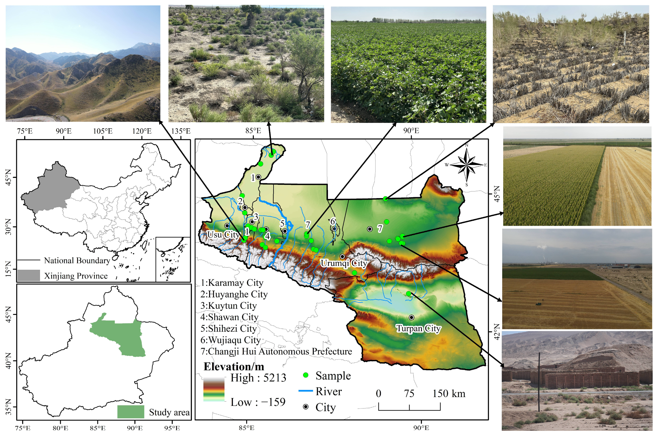
Figure 1. Map of the study area.
Agronomy 15 02704 g001
Figure 2. Research framework.
Agronomy 15 02704 g002
Figure 3. Causal Feedback Diagram of Land-Use Demand Change Based on the SD Model. “+” indicates a positive relationship, and “−” indicates a negative relationship.
Agronomy 15 02704 g003
Figure 4. Spatial Distribution of Land-Use Types and Area Proportions of Each Type from 2000 to 2020. (a) 2000, (b) 2005, (c) 2010, (d) 2015, (e) 2020.
Agronomy 15 02704 g004
Figure 5. Predicted Land-Use Distribution Patterns under Different Scenarios. (a) SSP119-2030, (b) SSP119-2040, (c) SSP119-2050, (d) SSP245-2030, (e) SSP245-2040, (f) SSP245-2050, (g) SSP585-2030, (h) SSP585-2040, (i) SSP585-2050. A, B, and C indicate the zoomed areas selected for detailed analysis.
Agronomy 15 02704 g005
Figure 6. Comparison of Probability Density Distributions of HQ and RSEI. (a) 2000, (b) 2005, (c) 2010, (d) 2015, (e) 2020.
Agronomy 15 02704 g006
Figure 7. Spatial Distribution of HQ from 2000 to 2020. (a) 2000, (b) 2005, (c) 2010, (d) 2015, (e) 2020.
Agronomy 15 02704 g007
Figure 8. Spatial Distribution of HQ under Different Scenarios. (a) SSP119-2030, (b) SSP119-2040, (c) SSP119-2050, (d) SSP245-2030, (e) SSP245-2040, (f) SSP245-2050, (g) SSP585-2030, (h) SSP585-2040, (i) SSP585-2050. A, B, and C indicate the zoomed areas selected for detailed analysis.
Agronomy 15 02704 g008
Figure 9. Spatiotemporal dynamics and Sankey representation of HQ (2020–2050) under different scenarios. (a) SSP119, (b) SSP245, (c) SSP585. A, B, and C indicate the zoomed areas selected for detailed analysis.
Agronomy 15 02704 g009
Figure 10. Spatial distribution of the coefficient of variation (CV) of HQ predictions under multiple future scenarios for 2030, 2040, and 2050.
Agronomy 15 02704 g010
Figure 11. OMGD Driving Force Analysis Results. (a): Single-Factor Detection Result, (b): Factor Interaction Detection Result. (Note: kms, jnb, gsm, qt denote K-means, natural breaks, Gaussian mixture model stratification methods, quantiles).
Agronomy 15 02704 g011
Table 1. Data sources.
DataApplicationPeriodResolutionData Source
Gross domestic product (GDP)PLUS, OMGD2000–20201 kmResource and Environment Science Data Platform
(https://www.resdc.cn/)
Population density (POP)PLUS, OMGD2000–20201 km
Normalized difference vegetation index (NDVI)OMGD2000–202030 m
Soil typePLUS/1 km
RiverPLUS2019/National catalog Service For Geographic Information
(https://www.webmap.cn/)
Level 1 roadPLUS2019/
Level 2 roadPLUS2019/
Level 3 roadPLUS2019/
HighwayPLUS2019/
RailwayPLUS2019/
GovernmentPLUS2019/
Elevation (DEM)PLUS, OMGD/30 mGeospatial Data Cloud
(https://www.gscloud.cn/)
SlopePLUS/30 m
Nighttime light dataOMGD2000–20201 kmNational Tibetan plateau Data center (https://data.tpdc.ac.cn/)
TemperaturePLUS, OMGD2000–20201 km
PrecipitationPLUS, OMGD2000–20201 km
Livestock DensityOMGD2000–20201 kmThe Food and Agriculture Organization (https://data.apps.fao.org/)
Table 2. Habitat suitability and sensitivity.
Land-Use TypeHabitat SuitabilitySensitivity
Cultivated LandConstruction LandUnused LandHighwayRailway
Cultivated Land0.20.10.90.40.50.5
Forest10.50.80.70.80.9
Grassland10.50.70.40.70.7
Water0.90.40.70.50.70.8
Construction Land000000
Unused Land000000
Table 3. Impact distance and weight of threat factors.
Threat FactorsMax_Dist (km)WeightDecay Type
Cultivated Land30.5Linear
Construction Land80.8Exponential
Unused Land40.4Linear
Highway50.5Linear
Railway60.6Linear
Table 4. Correlation and spatial statistics of RSEI and HQ.
20002005201020152020
MetricValuep-ValueValuep-ValueValuep-ValueValuep-ValueValuep-Value
Pearson r0.375 00.328 00.345 00.367 00.329 0
Spearman ρ0.530 00.507 00.466 00.457 00.446 0
Moran’s I (RSEI)0.785 0.0010.785 0.0010.791 0.0010.855 0.0010.846 0.001
Moran’s I (HQ)0.941 0.0010.941 0.0010.942 0.0010.942 0.0010.942 0.001
Disclaimer/Publisher’s Note: The statements, opinions and data contained in all publications are solely those of the individual author(s) and contributor(s) and not of MDPI and/or the editor(s). MDPI and/or the editor(s) disclaim responsibility for any injury to people or property resulting from any ideas, methods, instructions or products referred to in the content.