You are currently viewing a new version of our website. To view the old version click .
Agronomy
  • Article
  • Open Access

31 October 2025

Quantifying Grazing Intensity from Aboveground Biomass Differences Using Satellite Data and Machine Learning

,
,
,
,
,
and
1
Grassland Research Institute, Chinese Academy of Agriculture Sciences, Hohhot 010010, China
2
Forestry and Grassland Monitoring and Planning Institute of Inner Mongolia, Hohhot 010020, China
3
Inner Mongolia Forestry Science Research Institute, Hohhot 010020, China
*
Author to whom correspondence should be addressed.
This article belongs to the Section Precision and Digital Agriculture

Abstract

Accurately quantifying grazing intensity (GI) is crucial for assessing grassland utilization and supporting sustainable management. Traditional livestock-based approaches cannot capture the spatial heterogeneity of grazing or its dynamic response to climate variability. The objective of this study was to develop a remote sensing-based quantitative framework for estimating GI across the Inner Mongolian grasslands. The framework integrates MODIS vegetation indices, ERA5-Land climate variables, topographic factors, and field-measured data and GI was quantified as the proportional difference between potential and satellite-derived aboveground biomass (AGB), providing a spatially explicit measure of forage utilization. In this framework, potential AGB (AGBp) represents the climate-driven growth capacity under ungrazed conditions reconstructed using machine learning models, whereas satellite-derived AGB (AGBs) denotes the standing AGB remaining under current grazing pressure. Validation using 324 paired grazed–ungrazed plots demonstrated strong agreement between modeled and observed GI (R2 = 0.65, RMSE = 0.18). This AGB-difference-based approach provides an effective and scalable tool for large-scale rangeland monitoring, offering quantitative insights into grass–livestock balance, ecological restoration, and adaptive management in arid and semi-arid regions.

1. Introduction

Globally, grasslands constitute one of the most extensive terrestrial biomes, covering more than one-third of the Earth’s land surface and supporting over 1.4 billion ruminants [1,2,3,4]. By sustaining forage production and regulating biogeochemical cycles, grasslands not only secure global food and fiber supply but also deliver essential ecosystem services [5]. These include provisioning services such as forage and livestock products and regulating and supporting services that enhance soil carbon storage, water conservation, and biodiversity maintenance, together underpinning ecological stability in arid and semi-arid regions [2,6,7]. In China’s Inner Mongolia, grasslands carry additional strategic significance: they underpin pastoral livelihoods while serving as a key ecological barrier that safeguards northern China from desertification and climate risks [8,9,10,11]. Yet these ecosystems are increasingly threatened by the combined impacts of intensive grazing and ongoing climate change, particularly in semi-arid steppe regions, where degradation processes unfold rapidly and ecosystem functions are severely compromised [6,12,13]. This context highlights the urgent need for precise, spatially explicit assessments of GI and its temporal evolution, which are critical for maintaining a balance between forage supply and livestock demand, promoting ecological restoration, and guiding sustainable rangeland governance in northern China [14,15].
Traditional approaches to GI assessment have typically relied on livestock census data, assuming that animal numbers directly translate into grazing pressure [16,17,18]. However, this assumption has multiple flaws. First, livestock statistics seldom differentiate between stall-fed animals and those grazing freely on natural pastures, which weakens the ecological relevance of census-based indicators and produces nonlinear or distorted relationships between animal counts and grassland utilization [19,20]. Second, such statistics are usually aggregated at county or prefectural scales and reported annually, resulting in poor spatial granularity and delayed availability [21,22]. Third, management practices such as seasonal rest grazing, rotational systems, and grazing bans vary widely across regions [21,23], further decoupling livestock inventories from the actual pressure exerted on the land. These limitations highlight the need for alternatives that directly capture the realized utilization of forage resources rather than relying solely on animal numbers. In addition, some studies have employed GPS-based livestock tracking to estimate GI from animal movement data [22,24]. This method can directly record grazing trajectories and durations, providing fine-scale information on pasture use. However, its application remains limited due to high equipment costs, battery endurance, device maintenance requirements, and potential impacts on animal health [18,24]. Overall, while GPS tracking improves the ground-level quantitative accuracy of GI estimation, it still faces major constraints in conducting long-term, large-scale, and operational grazing monitoring.
Remote sensing offers a powerful solution because it provides consistent, large-scale, and temporally frequent observations of vegetation status [25,26,27,28]. Yet, vegetation indices (VIs) derived from satellite imagery integrate both climatic influences and grazing effects [15,19,29,30], making it difficult to isolate the grazing signal. To address this, researchers have proposed reconstructing potential vegetation indices (VIp) that represent ungrazed, climate-driven productivity [31]. A persistent challenge, however, is that numerous vegetation indices exist, and it remains unclear which most reliably reflects baseline productivity under ungrazed conditions [32].
Machine learning (ML) techniques have increasingly been applied to grassland monitoring to disentangle climate-driven variability from grazing effects [33,34]. Algorithms such as random forests, boosting trees, and deep neural networks can capture nonlinear vegetation–climate relationships more effectively than traditional regression methods [25,29,35]. Nevertheless, these models differ in their interpretability, computational demands, and sensitivity to data structure [25,36]. No consensus yet exists on which ML approach is best suited for reconstructing VIp or for deriving GI consistently across large regions [25,37]. Understanding the strengths, limitations, and performance boundaries of different machine learning algorithms is therefore essential for reliably separating climatic influences from grazing impacts and for enabling high-resolution monitoring of GI. Another factor influencing model performance is the choice of spatial stratification. Subdividing training data by ecological zones or administrative units can reduce parameter heterogeneity, improve predictive stability, and enhance ecological interpretability [25,38,39]. If zoning is too coarse, critical differences among ecosystems may be lost, while overly fine partitions can lead to sample sparsity and overfitting. However, the relative merits of different subdivision strategies for reconstructing VIp and estimating GI remain underexplored, limiting progress toward spatially adaptive monitoring [40].
Inner Mongolia, one of China’s most important pastoral regions, faces accelerating degradation due to fragile ecosystems and long-term grazing pressure [9]. Yet a high-resolution, long-term dataset of GI is still lacking, constraining both ecological research and management decision-making. This study addresses these gaps by proposing a remote sensing-driven framework that defines GI as the proportional difference between AGBp and AGBs. Unlike census-based methods, this definition directly reflects the actual utilization of grassland production. Specifically, our objectives are to achieve the following:
  • Identify the optimal combination of VIs, ML algorithms, and ecological zoning strategies for reconstructing VIp.
  • Derive AGBp and AGBs from 2000 to 2024 and calculate GI as their proportional difference.
  • Analyze the spatiotemporal dynamics of GI across Inner Mongolia and evaluate its implications for grass–livestock balance and sustainable rangeland management.
By combining machine learning, remote sensing, and field validation, this work delivers a high-resolution, operational, and cost-effective dataset for monitoring GI, offering new insights and practical tools for grassland conservation and governance in northern China

2. Materials and Methods

2.1. Study Area

The study was conducted across the grasslands of Inner Mongolia, northern China (Figure 1), a region shaped by a temperate continental monsoon climate [11]. Mean annual temperature (MAT) decreases from about 9 °C in the arid southwest to nearly −5 °C in the humid northeast, while mean annual precipitation (MAP) ranges from 40 to 580 mm, with more than 80% concentrated between May and October. The landscape is dominated by plateau terrain—including the Ordos, Xilingol, and Hulunbuir plateaus—generally rising to around 1000 m above sea level.
Figure 1. Study area, AGB sampling sites, and hierarchical regional subareas. The map shows the distribution of grasslands and AGB sampling sites, along with the hierarchical ecological divisions including Groups, Subgroups, Types, and County-levels boundaries. Different colors indicate different hierarchical regional subareas.
Vegetation composition reflects the strong precipitation gradient and can be broadly classified into three steppe types from west to east. The desert steppe, occurring under minimal rainfall, supports sparse vegetation and is highly vulnerable to degradation. The typical steppe in the central zone is dominated by Leymus chinensis and Stipa grandis, while the more humid meadow steppe in the east is characterized by species such as Stipa baicalensis and Filifolium sibiricum. As one of China’s largest pastoral regions, Inner Mongolia sustains intensive livestock grazing, mainly by sheep and cattle [22]. Inner Mongolia’s grassland husbandry is dominated by extensive free grazing, but the system has undergone substantial institutional change since the 1980s [41,42]. Following the household contract reform of grassland tenure, most pastures were divided and fenced at the household level, which has largely restricted the movement of wild herbivores except in border or protected areas. Since the enactment of the Grassland Law in 1985, reclamation and conversion of grasslands for cropland, mining, or other land uses have been strictly prohibited, ensuring that grazing and hay harvesting remain the primary modes of land utilization [42]. To avoid early mowing that could reduce seed availability and hinder vegetation regeneration, hay harvesting in most parts of Inner Mongolia is usually concentrated between mid- and late August each year [42]. Because our study focuses on vegetation conditions in mid-August, before the main mowing period, it can be reasonably assumed that grazing is the dominant factor driving vegetation changes in Inner Mongolia.

2.2. Data Usage

2.2.1. Satellite Data

The MODIS 8-day surface reflectance product (MOD09A1) was obtained via the Google Earth Engine (GEE) platform (Google LLC, Mountain View, CA, USA)., which has three reflectance bands, blue (459−479 nm), red (620−670 nm), and near-infrared (841−876 nm), at a spatial resolution of 500 m, from 2000 to 2024 were used for this study. These bands were used to calculate vegetation indices required for model input, as detailed in Table 1. To ensure data quality and temporal consistency, invalid pixels were identified using the MOD09A1 quality control (QC) layer. Missing values were then gap-filled using valid observations within a ±48-day temporal window.
Table 1. Summary of 17 driving variables from five categories used for VIp reconstruction and AGB conversion across Inner Mongolia.

2.2.2. Regional Subareas Data

The data on grassland group, subgroup, and type reflect the spatial distribution patterns and structural composition of grassland resources in Inner Mongolia. Classification was based on a multi-factor approach integrating vegetation characteristics and habitat conditions, incorporating variables such as vegetation type, hydrothermal regimes, and topographic features (Figure 1, Table 1). The classification follows a minimum mapping unit of 4 m2, and the dataset was provided by the Inner Mongolia Forestry and Grassland Monitoring and Planning Institute.

2.2.3. Climatic Data

Climate data were derived from the ERA5-Land daily data generated by the Copernicus Climate Change Service at the European Centre for Medium-Range Weather Forecasts (https://cds.climate.copernicus.eu/, accessed on 15 October 2024). This data product provides daily meteorological data on a 0.1° (~10 km) latitude/longitude climate modeling grid. The band temperature_2m and total_precipitation_sum from 1980 to 2024 were used for this study. These daily records were then used to calculate the precipitation, temperature, MAP, MAT, precipitation anomaly (AP) and temperature anomaly (AT) over the 20-year period (1980–1999).

2.2.4. Topographical Data

Topographical data with a spatial resolution of 30 m, obtained from the National Aeronautics and Space Administration (NASA) (https://earthdata.nasa.gov/), were resampled to 500 m resolution using ArcGIS 10.8 software for further analysis.

2.2.5. Ground Observation Data

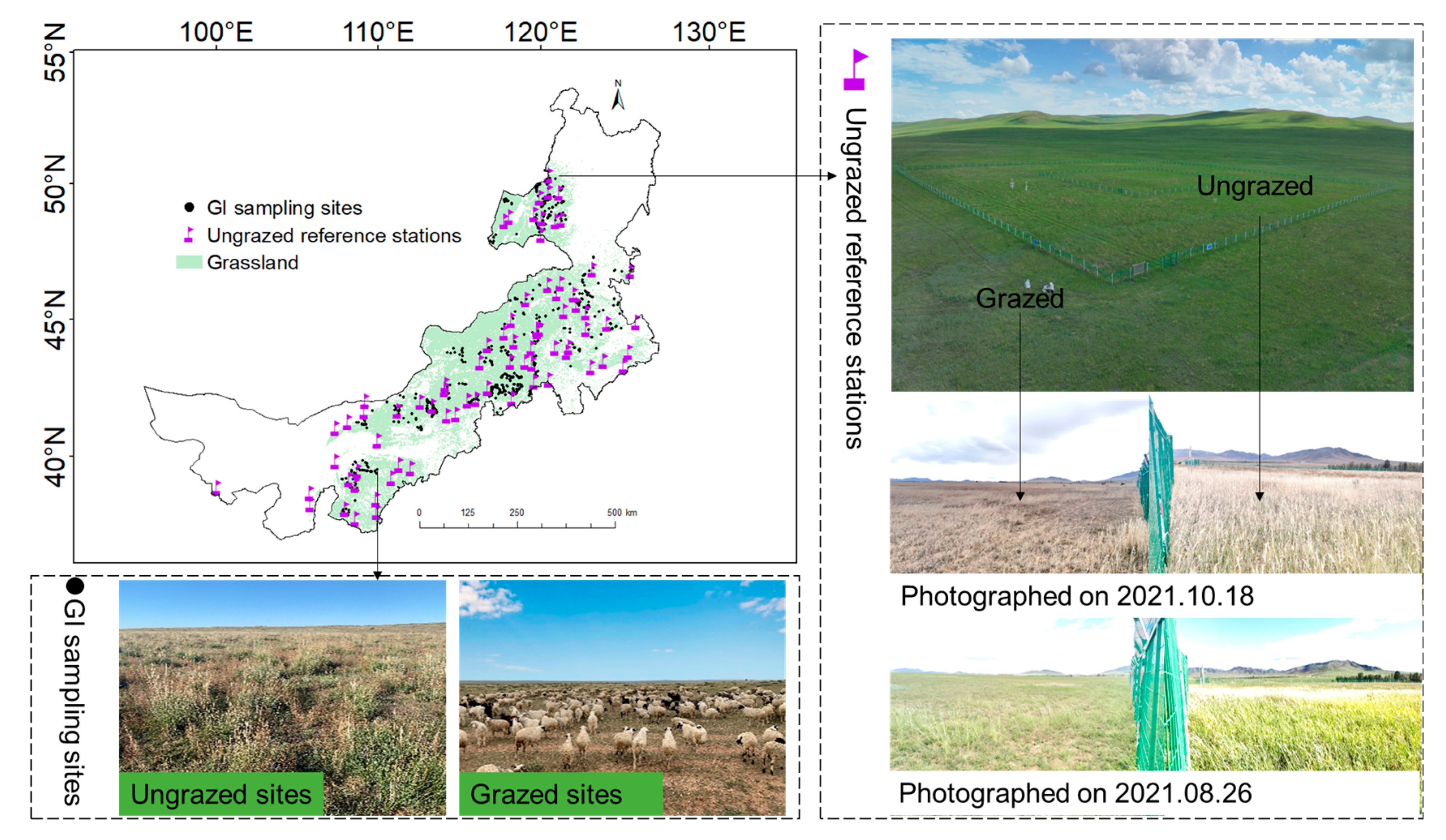
Ground observation datasets were used to support model training and validation, including AGB measurements, GI quadrats, and ungrazed reference stations (Figure 1 and Figure 2, Table 2).
Figure 2. Ground data network distribution and representative field sites. Black points denote GI sampling sites, where paired plots (grazed vs. ungrazed) were surveyed during the growing season. Purple flags indicate long-term ungrazed reference stations, established with seasonal grazing exclusion. Field photographs illustrate contrasts in vegetation between grazed and ungrazed plots, highlighting differences in biomass residuals under grazing exclusion.
Table 2. Summary of ground observation datasets used for VIp reconstruction, AGB conversion, and GI estimation in this study.
The measurements of AGB were derived from the National Inventory of Grassland Resources by the National Forestry and Grassland Administration of Inner Mongolia from 2020 to 2024 (http://www.forestry.gov.cn), and a total of 2789 field plots were collected during the peak growing season (July–August) (Figure 1). The sampling followed a stratified design, with plots evenly distributed across major grassland types to ensure representative coverage of vegetation and environmental gradients. Each plot was treated as an independent sample for analysis. The AGB was measured by harvesting the aboveground portion of the plants and oven-drying them to obtain the dry mass weight.
The GI quadrats were collected from grazed and ungrazed plots by comparing vegetation residuals within adjacent areas (<1 km apart), and 648 field plots were surveyed during the peak growing season (July–August) (Figure 2). The different GI levels of adjacent samples were primarily driven by grazing activities, as neighboring plots typically had similar climates and environments. The enclosed plots without livestock grazing were selected as the ungrazed samples. Then, using the ungrazed samples as benchmarks in paired sampling, the GI of other plots was determined based on the reduction rates of vegetation coverage, grass height, edible forage, and residual biomass [49]. Following the national standard Evaluating Criterion for Balance of Forage Supply and Livestock Requirement (LY/T 3320–2022) issued by the National Forestry and Grassland Administration, GI levels were classified as light, moderate, and heavy according to the ratio of grazed to ungrazed values for vegetation cover, height, and AGB, with reductions of <20%, 21–30%, and >30%, respectively. When the three indicators indicated different grades, the AGB-based level was adopted as the representative GI [49].
These evaluation criteria based on vegetation residuals are unaffected by grassland type and climate zone and represent a more practical approach than that based only on livestock number for grassland management. This approach assumes that differences in vegetation residuals between paired grazed and ungrazed plots are primarily caused by livestock grazing rather than by vegetation type or climatic gradients. Because each paired plot was located within a short distance (<1 km) and shared similar topography, soil, and climatic conditions, the effect of regional grassland types and climate zones on the residual-based evaluation criteria was minimized. Therefore, the derived GI mainly reflects grazing-induced vegetation reduction rather than environmental variability.
The ungrazed reference stations were established by the Forestry and Grassland Monitoring and Planning Institute of Inner Mongolia and are evenly distributed across the region’s major grassland types (Figure 2). Most of the plots were set up around 2020, with an area of 2−3.3 hectares each. Grazing has been strictly excluded within these sites, making them representative of ungrazed vegetation conditions.

2.3. Research Methods

To quantify GI from an ecological perspective, this study developed an integrated framework that combines multi-source remote sensing, climate reanalysis, topographic information, and field-based observations (Figure 3). The framework utilizes both VIs derived from MODIS imagery and reconstructed VIp representing ungrazed and climate-driven vegetation baselines. It comprises three main components: (1) reconstruction of VIp using climate and topographic predictors, (2) machine-learning-based estimation of AGB (AGBp and AGBs) under grazing-free and grazed conditions, and (3) calculation of GI as a dimensionless indicator of vegetation utilization, followed by spatiotemporal trend analysis. Unlike conventional livestock-based approaches, this framework explicitly links vegetation productivity with climatic and topographic constraints, enabling ecologically meaningful and spatially explicit quantification of GI across heterogeneous grassland environments.
Figure 3. Overall technical framework of this study. The framework includes three main steps: (1) reconstruction of VIp using ungrazed reference sites and multiple machine-learning models; (2) conversion of VIp to AGBp; and (3) estimation of GI and spatiotemporal pattern analysis.

2.3.1. Reconstruction of VIp

VIp representing ungrazed and climate-driven vegetation states, were reconstructed to describe the potential vegetation productivity unaffected by grazing disturbances. The reconstruction was based on long-term ungrazed reference plots (n = 76; Figure 2) that serve as ecological baselines. MODIS-derived vegetation indices (NDVI, EVI, EVI2, SAVI, and NIRv) were combined with concurrent temperature and accumulated precipitation over multiple lag periods (0−72 days) extracted from the ERA5-Land dataset to capture delayed vegetation responses to climatic drivers.
To model the climate–vegetation relationships, six machine-learning algorithms—Random Forest (RF), Gaussian Process Regression (GPR), Least Squares Boosting (LSBoost), Support Vector Machine (SVM), Multiple Linear Regression (MLR), and Elastic Net Regression (ENET)—were evaluated and compared (Table 3). These models were trained under multiple ecological stratifications, including grassland class, subclass, type, administrative division, and pixel-level domains, to account for spatial heterogeneity in vegetation–climate interactions.
Table 3. Summary of Machine Learning Algorithms.
Model training adopted both hold-out (70/30 split) and five-fold cross-validation schemes, using R2 and RMSE as primary evaluation metrics. For each subregion, the model with the best performance was selected to generate spatially continuous VIp predictions. This multi-model and stratified approach ensured that the reconstructed VIp accurately reflected potential vegetation productivity across diverse climatic and ecological gradients, providing a consistent ungrazed baseline for subsequent AGB modeling.

2.3.2. AGB Conversion

AGB was estimated through a unified RF regression framework designed to capture the nonlinear response of vegetation productivity to climatic and topographic factors. The model integrated vegetation indices, climatic anomalies (AT, AP), long-term climate means (MAT, MAP), and topographic variables derived from the digital terrain model (DTM). Both DEM and slope were initially tested as potential predictors. However, variable importance analysis (Figure S1) showed that DEM contributed substantially more than slope, and the two variables exhibited strong collinearity. Therefore, only DEM was retained in the final model to avoid redundancy and ensure model stability.
Two biomass states were simulated independently:
(1)
AGBp—potential biomass estimated from reconstructed VIp, representing vegetation growth capacity under ungrazed and climate-constrained conditions;
(2)
AGBs—remaining biomass derived from observed VIs, representing vegetation conditions after grazing disturbance.
The model formulation can be expressed as:
AGB   =   ML ( AT ,   AP ,   MAT ,   MAP ,   VI ,   DEM )
where ML denotes the machine learning-based Random Forest regression model; AT represents temperature anomaly; AP represents precipitation anomaly; MAT is mean annual temperature; MAP is mean annual precipitation; DEM represents elevation derived from topographic data.
AGB model training employed a combination of holdout validation and 5-fold cross-validation. Specifically, 10% of the samples were reserved for independent validation, while the remaining 90% were used for iterative training [25]. Within each iteration, four out of five data subsets were used for training and the fifth for validation, rotating through all subsets. This procedure was repeated four times, and average validation errors were computed across both holdout and cross-validation datasets. Finally, given the availability of ground-truth AGB data, the model was retrained on the entire dataset using 5-fold cross-validation to produce the final AGB upscaling models.

2.3.3. Grazing Intensity Estimation and Spatiotemporal Analysis

GI was defined as a dimensionless ratio between AGBp and AGBs. GI ranges from 0 to 1 and reflects the extent to which grassland productivity has been utilized. The GI value of 0 indicates no grazing, where the retention biomass equals the capacity biomass (AGBs = AGBp). The GI value of 1 represents complete vegetation removal, where the retention biomass is zero (AGBs = 0). Intermediate values indicate varying levels of utilization, with values closer to 0 reflecting low GI and values closer to 1 indicating high GI.
GI is calculated as follows:
GI = AGBp AGBs AGBp
This formulation quantifies the proportion of vegetation consumed and serves as a standardized measure for assessing grazing pressure across spatial and temporal gradients.
To describe the overall temporal evolution of GI, an ordinary least squares (OLS) regression was applied to the regional mean GI time series (2000−2024), with year as the independent variable. The regression slope represented the rate of change over time. The Hurst exponent (H) was further calculated to evaluate the long-term persistence of the series. H values close to 0.5 indicated weak temporal dependence, suggesting that autocorrelation had little influence on the OLS-derived trend.
To characterize the spatially distributed temporal trends, the non-parametric Theil–Sen median slope estimator and Mann–Kendall test were applied at the pixel level to quantify the magnitude, direction, and significance of GI changes. This combined approach enables robust detection of both significant increases and decreases in GI while minimizing the influence of non-normality, outliers, and potential temporal dependence.

2.3.4. Validation and Accuracy Assessment

The reliability of remote sensing-derived GI was evaluated using 648 GI plots collected during the peak growing season. Field-based GI was calculated as the relative difference in AGB between paired plots. Model estimates were compared against these field values, with R2, RMSE, and MSE used as evaluation metrics. Additionally, Pearson’s correlation coefficients were calculated to assess feature–response relationships. Higher R2 and lower error values were interpreted as improved model performance. The formulas for these evaluation metrics are as follows:
R 2 = 1 i = 1 n y i ^ y i 2 i = 1 n y i y ¯ 2
R M S E = i = 1 n y i ^ y i 2 n
where y i is the observed value, y i ^ is the predicted value, y ¯ is the mean of the observed values, and n is the sample size.

3. Results

3.1. Importance of Driving Variables

Five commonly used vegetation indices—NDVI, EVI, EVI2, NIRv, and SAVI—were reconstructed under grazing-free conditions to evaluate the influence of different climate driver combinations on model performance. The candidate predictor variables included multi-scale lagged precipitation and concurrent air temperature.
The five vegetation indices demonstrated varying sensitivities to these climatic drivers. NDVI achieved the highest reconstruction accuracy (R2 = 0.545) when driven by a combination of 32-day lagged precipitation and concurrent temperature. EVI2 and SAVI performed slightly less accurately, while EVI showed the weakest performance.
Considering both model robustness and consistency in input–response relationships, potential NDVI (NDVIp) was selected as the core vegetation index for estimating GI. The optimal configuration was based on 32-day lagged precipitation and concurrent temperature (Figure 4).
Figure 4. Reconstruction accuracy of different vegetation indices across precipitation-lag windows based on RF. The asterisk (*) indicates the highest reconstruction accuracy among lag windows for vegetation index.

3.2. Performance of the ML Models

Six machine learning algorithms—RF, GPR, LSBoost, SVM, MLR, and ENET—were evaluated using the top three combinations of climate drivers for NDVIp reconstruction. As shown in Figure 5, RF achieved the highest predictive accuracy (R2 = 0.545) and the lowest RMSE, indicating strong model performance in capturing vegetation dynamics under ungrazed conditions. GPR (R2 = 0.544) and SVM (R2 = 0.541) performed comparably, albeit with slightly higher errors. In contrast, LSBoost, MLR, and ENet exhibited reduced accuracy (R2 < 0.49) and greater variability across samples. Among the three algorithms with comparable predictive accuracy (RF: R2 = 0.545, GPR: R2 = 0.544, and SVM: R2 = 0.541), RF demonstrated substantially higher computational efficiency, with training time reduced by more than half compared with GPR and SVM. Considering both accuracy and efficiency, RF was therefore selected as the foundational model for subsequent grazing-intensity estimation.
Figure 5. Predictive accuracy of six regression models for NDVIp. The black dashed line represents the 1:1 reference line, and the black solid line represents the fitted regression line.

3.3. Effect of Spatial Stratification on Model Performance

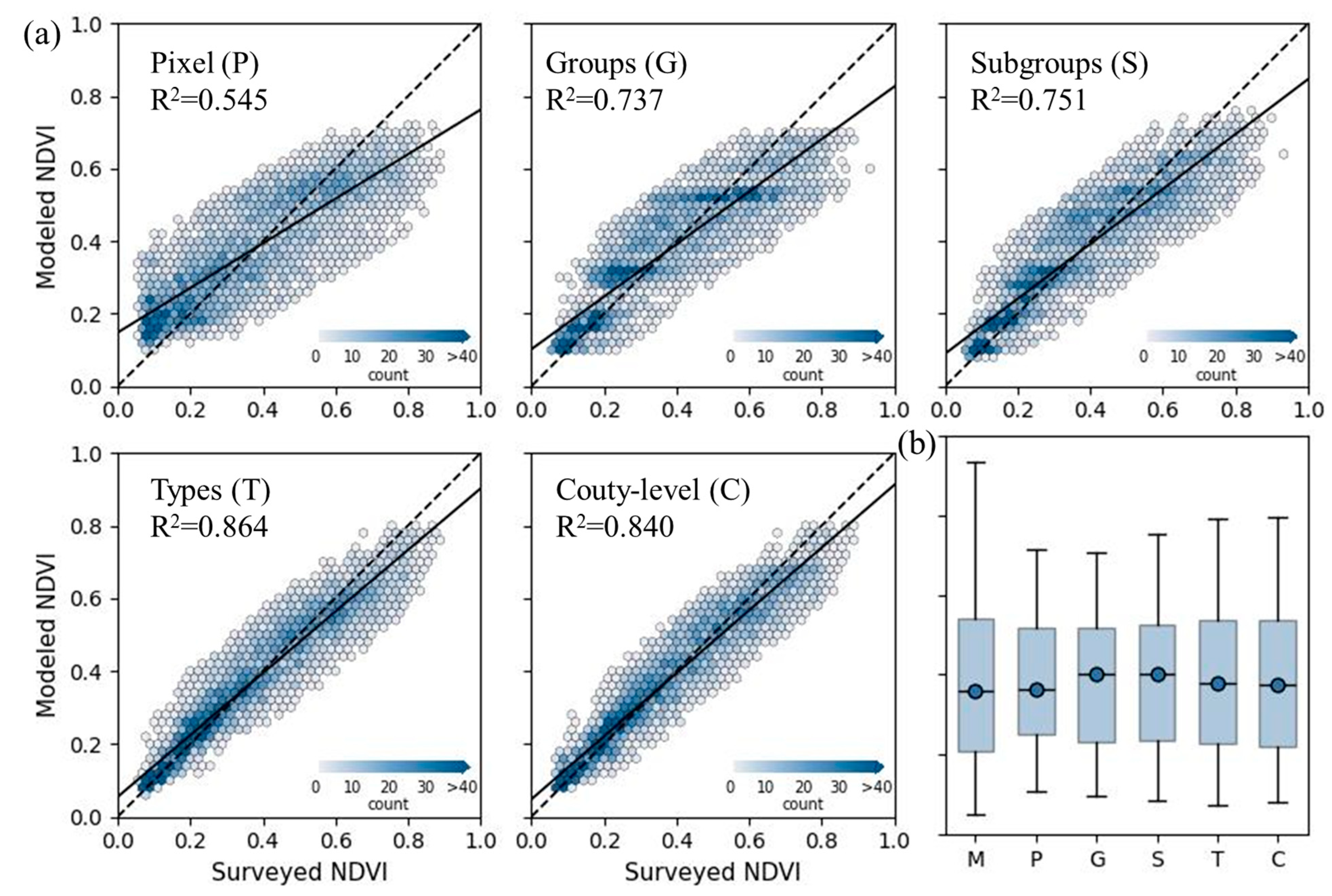
To assess the influence of ecological and administrative stratification on model accuracy, five spatial zoning schemes were compared: pixel-level, vegetation group, subgroup, type, and county-level divisions. As shown in Figure 6a, stratification significantly improved the NDVIp model’s predictive accuracy across all schemes. Among them, type-level stratification yielded the highest coefficient of determination (R2 = 0.864) and the lowest RMSE, followed closely by county-level (R2 = 0.840) and subgroup-level (R2 = 0.751) partitions. In contrast, pixel-based modeling performed the worst (R2 = 0.545), likely due to high variability and sample sparsity. The performance ranking of zoning strategies was: type > county > subgroup > group > pixel. These results suggest that aligning model training with ecologically homogeneous units (e.g., vegetation types) enhances generalization by reducing within-group variability. As shown in Figure 6b, type-level stratification also minimized prediction error dispersion, further demonstrating its superiority for spatially adaptive modeling.
Figure 6. (a) Scatterplots of modeled versus surveyed NDVIp under five spatial partition strategies: pixel (P), group (G), subgroup (S), type (T), and county-level (C). The dashed line represents the 1:1 reference, and the solid line shows the fitted regression; (b) boxplots of prediction errors for each strategy, with the central line denoting the median and the dots representing the mean values.

3.4. Quantitative Estimation of Grazing Intensity

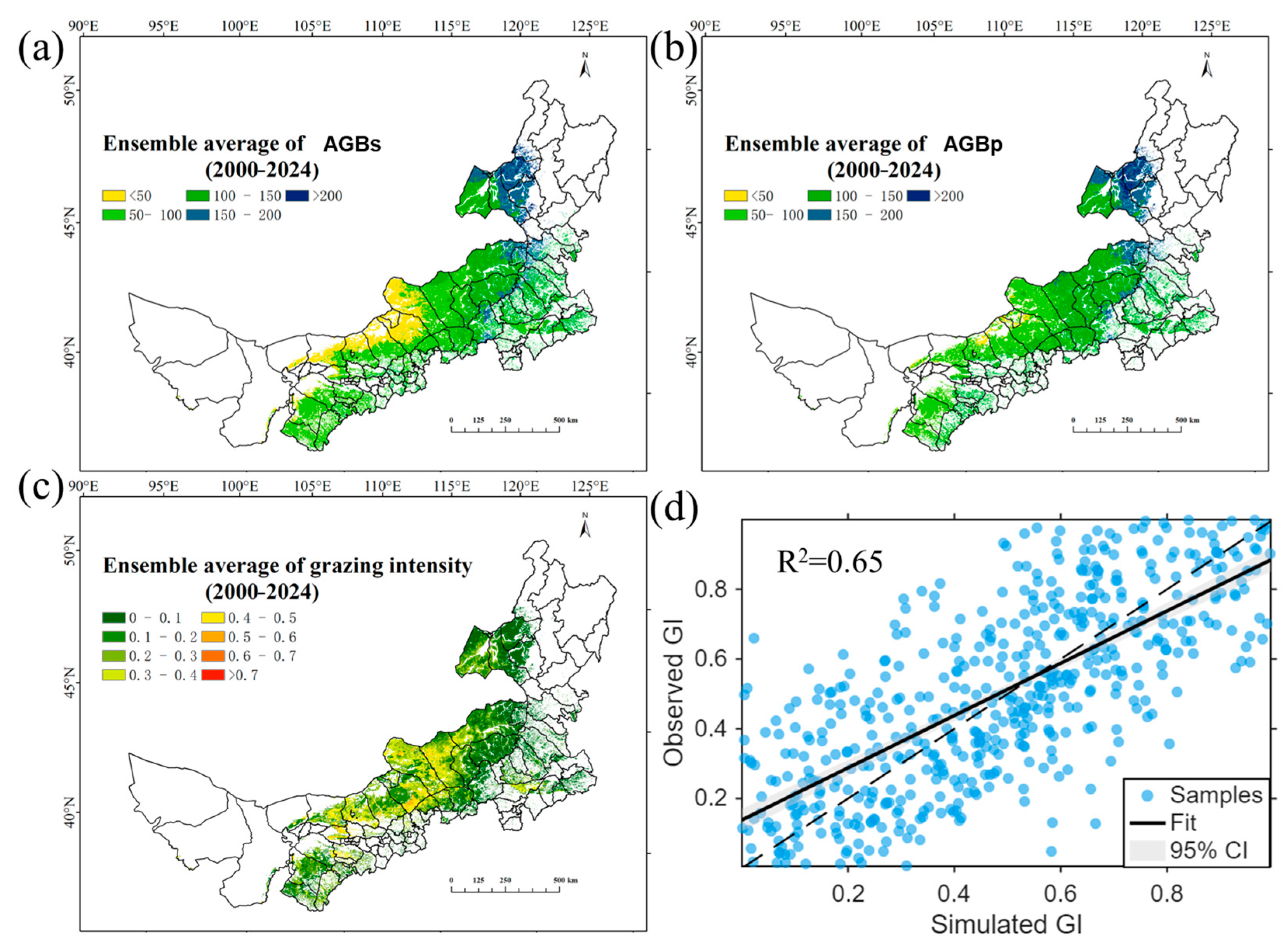
Using the optimal driver combination—concurrent temperature and 32d lagged precipitation—identified by the Random Forest model stratified by type, NDVIp was reconstructed and integrated into a biomass model to simulate AGBp and AGBs. The model achieved R2 values of 0.76 for AGBs and 0.69 for AGBp. The derived GI yielded a validation R2 of 0.65 against observed values, with no systematic bias and uniformly distributed residuals, confirming its robustness for spatiotemporal analysis (Figure 7d).
Figure 7. Spatial distribution: (a) AGBs; (b) AGBp; (c) GI; (d) validation of GI simulated. The dashed line represents the 1:1 reference, and the solid line shows the fitted regression.
In terms of spatial patterns, AGBs showed a more moderate gradient, with notable reductions in central and eastern regions due to grazing pressure. In contrast, AGBp exhibited a clear west-to-east increasing trend, with the highest values (>200 g·m−2) concentrated in the northeastern meadow steppes and forest-steppe transition zones. The spatial distribution of GI revealed relatively low intensity (<0.3) in the western desert steppes, moderate levels (0.3–0.5) in central typical steppes, and high GI (>0.6) primarily in the southeastern agro-pastoral ecotones. These patterns highlight the spatial heterogeneity of grazing impacts (Figure 7a–c).

3.5. Characterization of the Spatiotemporal Evolution of the Grassland Grazing Intensity

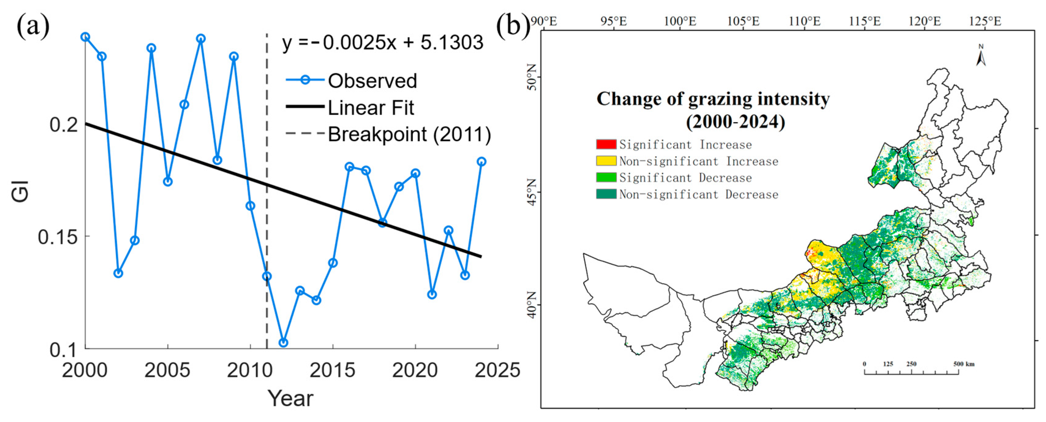
The overall declining trend of annual GI from 2000 to 2024 was well fitted by the OLS regression, and the Hurst exponent (H ≈ 0.52) suggested weak persistence, indicating that temporal autocorrelation had little influence on the observed trend. From 2000 to 2024, the overall GI in Inner Mongolia grasslands exhibited a declining trend, with an average annual decrease of approximately 1.2% (Figure 8a). A clear structural breakpoint was detected in 2011, after which GI values significantly dropped and stabilized at a relatively lower level, indicating a shift in grazing management or climate constraints.
Figure 8. Spatiotemporal Dynamics of GI in Inner Mongolian Grasslands, 2000−2024; (a) Mean GI time series for 2000−2024 with a breakpoint at 2011; (b) spatial trend categories derived from Theil-Sen slopes and Mann–Kendall tests, classified as significant increase, non-significant increase, significant decrease, and non-significant decrease.
Given that each pixel’s temporal trend was estimated independently using the Theil–Sen and Mann–Kendall tests, and that ecological stratification by grassland type was applied to reduce spatial heterogeneity, spatial autocorrelation is expected to have minimal influence on the robustness of the results. Spatially, the central and western regions showed the most substantial reductions in cumulative GI, particularly in previously overgrazed areas, reflecting the effect of targeted restoration programs and policy interventions. In contrast, slight increases in GI were observed in some northeastern and transitional zones, though these changes remained within a limited range (Figure 8b). Across the east–west gradient, GI exhibited distinct regional characteristics. The western region, dominated by desert steppes, showed relatively minor changes, while the central region—mainly typical steppe—experienced a pronounced decrease. In contrast, the eastern region, characterized by meadow steppes, maintained relatively low GI levels with limited variation.

4. Discussion

4.1. Spatial Heterogeneity of Grazing Intensities

In this study, we developed a dynamic framework for estimating GI by integrating remotely sensed NDVI data with field-measured AGB from both grazed plots and long-term ungrazed reference sites. In the study area, pastures have been fenced and contracted to households since the 1980s, grassland conversion has been legally prohibited since 1985, and hay mowing typically occurs in mid- to late August [42]. These management measures restrict the movement of wild herbivores, prevent large-scale land-use changes such as reclamation or mining, and thereby minimize non-grazing disturbances to vegetation dynamics. We therefore evaluated vegetation in mid-August, before the main mowing period, so that observed differences most likely reflect livestock grazing, while potential contributions from wild herbivores or other land-use disturbances are minimized. By incorporating a diverse set of ecological drivers, including vegetation type, climatic variables, and topographic features, our approach yields a more ecologically grounded and spatially explicit proxy for grazing pressure compared to traditional livestock-based assessments. In general, the multiyear average GI on Inner Mongolia increased from east to west during 2000 to 2024, with broad spatial heterogeneity. The average GI in Inner Mongolia from 2000 to 2024 was 0.15, suggesting that approximately 15% of AGB production was consumed by livestock annually during the growing season. Spatially, GI values were higher in the western desert steppe and eastern meadow steppe regions, and lower in the central typical steppe, revealing substantial regional heterogeneity. Temporal analysis revealed a weak but consistent declining trend (slope = −0.0025). This trend aligns with prior findings: [49] reported a decreasing pattern of GI based on grazing probability from 2015 to 2020, and [55] observed a similar long-term decline (2000−2022) using livestock statistics adjusted to reflect pressure on natural pastures (Figure 9). Although the methods differ in their definitions and magnitudes of GI, the convergence in trend underscores the robustness of our approach for characterizing grazing dynamics. Notably, a marked decline in GI was observed in 2011, which coincided with the initial implementation of Inner Mongolia’s ecological subsidy and grazing exclusion programs. This temporal correspondence suggests that these policies may have contributed to the reduction in grazing pressure, consistent with previous findings that reported similar policy effects in the region [56].
Figure 9. Comparison of simulated GI and independent livestock pressure indicators.
Overall, this study provides an accurate and spatially explicit assessment of GI by integrating biophysical variables and remote sensing indicators. The findings contribute to improved grassland monitoring, inform adaptive grazing management, and offer a scientific basis for policy-making in grassland conservation and restoration, thereby supporting the sustainable development of regional ecosystems.

4.2. Future Research Directions and Management Implications for Sustainable Grassland Development

This study generated a region-wide quantitative map of GI; however, the current spatial granularity is still insufficient to resolve micro-scale degradation patches or real-time livestock distribution [57]. Future work should therefore integrate high-resolution platforms—such as low-altitude UAVs and airborne LiDAR—with real-time animal-tracking technologies (e.g., GNSS collars and LoRa IoT tags) to create a “space–air–ground” multi-scale monitoring network. Coupling vegetation productivity and livestock activity through spatiotemporal data-assimilation algorithms would enable real-time identification of microscale overgrazed patches and grazing pathways, thereby providing the data foundation for precision management [16].
To promote sustainable utilization and fine-scale management of grassland resources, we propose a dynamic grass–livestock balancing strategy that leverages “grazing duration” as a regulatory lever. By combining the present grazing-intensity maps with industry or local overload thresholds, overstocked areas and their magnitudes can be spatially and quantitatively identified, facilitating targeted destocking. Recognizing that, under market conditions, destocking often takes the form of stall feeding rather than animal sale, we further convert the required destocking amount into an equivalent stall-feeding duration, enabling herders to estimate necessary fodder reserves and enhancing the operational feasibility and forward-looking nature of the management plan.
Overall, the proposed framework bridges the gap between ecological monitoring and operational management by enabling high-resolution, temporally explicit assessments of grazing pressure. Through the integration of remote sensing, machine learning, and ground-based validation, this approach offers a scalable and transferable tool to support sustainable grassland governance under changing climatic and socioeconomic conditions.

5. Conclusions

This study proposes an integrated, data-driven framework that combines remote sensing, climatic records, ground-based observations, and machine learning algorithms to generate high-resolution GI estimates across the Inner Mongolian grasslands. By reconstructing ungrazed vegetation baselines and quantifying the potential and observed AGB, the model enables monthly assessments of GI at a 500 m spatial resolution from 2000 to 2024—offering unprecedented insight into the spatiotemporal dynamics of grassland utilization. The results demonstrate strong agreement with field data and effectively capture the spatial heterogeneity and seasonal variability of grazing pressure. Compared to existing livestock census-based GI products, our model provides significantly improved accuracy, ecological relevance, and near-real-time monitoring capacity. These advances underscore the framework’s value as a scalable and transferable tool for rangeland monitoring, adaptive management, and early-warning systems. While the model exhibits strong predictive performance (R2 = 0.65), uncertainties persist—particularly with respect to meteorological variability and biomass response modeling—highlighting the need for further refinement. Nonetheless, the proposed approach contributes a robust foundation for spatializing GI and aligning grassland governance with principles of ecological sustainability, climate resilience, and food security. As grazing remains the dominant land use in arid and semi-arid ecosystems, high-resolution GI monitoring will be vital for supporting sustainable land management, ecological compensation schemes, and policy-making at the interface of agriculture and environmental protection.

Supplementary Materials

The following supporting information can be downloaded at https://www.mdpi.com/article/10.3390/agronomy15112537/s1. Figure S1: Variable importance ranking of predictors in the Random Forest model for AGB estimation. Figure S2: Interannual variation of potential (AGBp) and actual (AGBs) aboveground biomass.

Author Contributions

Conceptualization, A.L.; Data curation, Y.Y. and X.S.; Investigation, R.S., S.C., G.A. and X.Y.; Methodology, R.S. and A.L.; Software, R.S.; Writing—original draft, R.S. All authors have read and agreed to the published version of the manuscript.

Funding

This research was funded by the Natural Science Foundation of Inner Mongolia Autonomous Region (2023ZD04) and the Natural Science Foundation of Inner Mongolia Autonomous Region (2021MS03076).

Data Availability Statement

The data presented in this study are available from the corresponding author upon request. (The remote sensing datasets used in this study are publicly available from the Google Earth Engine platform. The field observation data are not publicly available due to institutional authorization requirements, but are available from the corresponding author upon reasonable request.).

Acknowledgments

The authors have reviewed and edited the output and take full responsibility for the content of this publication.

Conflicts of Interest

The authors declare no conflicts of interest.

Abbreviations

The following abbreviations are used in this manuscript:
AGBAboveground Biomass
AGBpPotential Aboveground Biomass
AGBsSatellite-Derived Aboveground Biomass
APPrecipitation Anomaly
ATTemperature Anomaly
DEMDigital Elevation Model
DTMDigital Terrain Model
ENETElastic Net Regression
GEEGoogle Earth Engine
GIGrazing Intensity
GPRGaussian Process Regression
HHurst Exponent
LSBoostLeast Squares Boosting
MAPMean Annual Precipitation
MATMean Annual Temperature
MLMachine Learning
MLRMultiple Linear Regression
NASANational Aeronautics and Space Administration
NDVINormalized Difference Vegetation Index
NIRvNear-Infrared Reflectance of Vegetation
OLSOrdinary Least Squares
QCQuality Control
RFRandom Forest
RMSERoot Mean Square Error
R2Coefficient of Determination
SAVISoil-Adjusted Vegetation Index
SRTMShuttle Radar Topography Mission
SVMSupport Vector Machine
UAVUnmanned Aerial Vehicle
VIVegetation Index
VIpPotential Vegetation Index
VIsSatellite-Observed Vegetation Indices

References

  1. Yu, Q.; Xu, C.; Wu, H.; Ke, Y.; Zuo, X.; Luo, W.; Ren, H.; Gu, Q.; Wang, H.; Ma, W.; et al. Contrasting drought sensitivity of Eurasian and North American grasslands. Nature 2025, 639, 114–118. [Google Scholar] [CrossRef]
  2. Zhu, J.; Zhang, Y.; Wu, J.; Zhang, X.; Yu, G.; Shen, Z.; Yang, X.; He, Y.; Jiang, L.; Hautier, Y. Herbivore exclusion stabilizes alpine grassland biomass production across spatial scales. Glob. Change Biol. 2024, 30, e17155. [Google Scholar] [CrossRef]
  3. MacDougall, A.S.; Esch, E.; Chen, Q.; Carroll, O.; Bonner, C.; Ohlert, T.; Siewert, M.; Sulik, J.; Schweiger, A.K.; Borer, E.T.; et al. Widening global variability in grassland biomass since the 1980s. Nat. Ecol. Evol. 2024, 8, 1877–1888. [Google Scholar] [CrossRef]
  4. Sha, Z.; Bai, Y.; Lan, H.; Liu, X.; Li, R.; Xie, Y. Can more carbon be captured by grasslands? A case study of Inner Mongolia, China. Sci. Total Environ. 2020, 723, 138085. [Google Scholar] [CrossRef]
  5. Bai, Y.; Cotrufo, M.F. Grassland soil carbon sequestration: Current understanding, challenges, and solutions. Science 2022, 377, 603–608. [Google Scholar] [CrossRef]
  6. Purevjav, A.-O.; Avirmed, T.; Wilcox, S.W.; Barrett, C.B. Climate Rather Than Overgrazing Explains Most Rangeland Primary Productivity Change in Mongolia. Science 2025, 389, 1229–1233. [Google Scholar] [CrossRef] [PubMed]
  7. Hu, T.; Cao, M.; Zhao, X.; Liu, X.; Liu, Z.; Liu, L.; Huang, Z.; Tao, S.; Tang, Z.; Guo, Y.; et al. High-Resolution Mapping of Grassland Canopy Cover in China through the Integration of Extensive Drone Imagery and Satellite Data. J. Photogramm. Remote Sens. 2024, 218, 69–83. [Google Scholar] [CrossRef]
  8. Zhou, T.; Yang, H.; Qiu, X.; Sun, H.; Song, P.; Yang, W. China’s grassland ecological compensation policy achieves win-win goals in Inner Mongolia. Environ. Res. Commun. 2023, 5, 031007. [Google Scholar] [CrossRef]
  9. You, C.; Wang, Y.; Tan, X.; Cui, E.; Zhang, B.; Bian, C.; Chen, B.; Xu, M.; Han, X.; Xia, J.; et al. Inner Mongolia grasslands act as a weak regional carbon sink: A new estimation based on upscaling eddy covariance observations. Agric. For. Meteorol. 2023, 342, 109719. [Google Scholar] [CrossRef]
  10. Wang, S.; Tuya, H.; Zhang, S.; Zhao, X.; Liu, Z.; Li, R.; Lin, X. Random forest method for analysis of remote sensing inversion of aboveground biomass and grazing intensity of grasslands in Inner Mongolia, China. Int. J. Remote Sens. 2023, 44, 2867–2884. [Google Scholar] [CrossRef]
  11. Sun, J.; Liu, W.; Pan, Q.; Zhang, B.; Lv, Y.; Huang, J.; Han, X. Positive legacies of severe droughts in the Inner Mongolia grassland. Sci. Adv. 2022, 8, eadd6249. [Google Scholar] [CrossRef]
  12. Xiang, Q.; Yu, H.; Huang, H.; Yan, D.; Yu, C.; Wang, Y.; Xiong, Z. The impact of grazing activities and environmental conditions on the stability of alpine grassland ecosystems. J. Environ. Manag. 2024, 360, 121176. [Google Scholar] [CrossRef]
  13. Zhang, M.; Delgado-Baquerizo, M.; Li, G.; Isbell, F.; Wang, Y.; Hautier, Y.; Wang, Y.; Xiao, Y.; Cai, J.; Pan, X.; et al. Experimental impacts of grazing on grassland biodiversity and function are explained by aridity. Nat. Commun. 2023, 14, 5040. [Google Scholar] [CrossRef]
  14. Li, C.; Zhou, W.; Fu, B.; Wang, S.; Ren, Z.; Hu, M.; Zhang, Y.; Rodriguez-Caballero, E.; Weber, B.; Stringer, L.C.; et al. Climate-driven ecological thresholds in China’s drylands modulated by grazing. Nat. Sustain. 2023, 6, 1363–1372. [Google Scholar]
  15. von Keyserlingk, J.; de Hoop, M.; Mayor, A.G.; Dekker, S.C.; Rietkerk, M.; Foerster, S. Resilience of vegetation to drought: Studying the effect of grazing in a Mediterranean rangeland using satellite time series. Remote Sens. Environ. 2021, 255, 112270. [Google Scholar]
  16. Wang, Z.; Lv, S.; Han, G.; Wang, Z.; Li, Z.; Ren, H.; Wang, J.; Sun, H.; Zhang, G. Heavy grazing reduced the spatial heterogeneity of Artemisia frigida in desert steppe. BMC Plant Biol. 2022, 22, 337. [Google Scholar] [CrossRef]
  17. Liu, J.; Isbell, F.; Ma, Q.; Chen, Y.; Xing, F.; Sun, W.; Wang, L.; Li, J.; Wang, Y.; Hou, F.; et al. Overgrazing, not haying, decreases grassland topsoil organic carbon by decreasing plant species richness along an aridity gradient in northern China. Agric. Ecosyst. Environ. 2022, 332, 112270. [Google Scholar] [CrossRef]
  18. Ma, Q.; Chai, L.; Hou, F.; Chang, S.; Ma, Y.; Tsunekawa, A.; Cheng, Y. Quantifying grazing intensity using remote sensing in alpine meadows on Qinghai-Tibetan Plateau. Sustainability 2019, 11, 417. [Google Scholar] [CrossRef]
  19. Yu, R.; Evans, A.J.; Malleson, N. Quantifying grazing patterns using a new growth function based on MODIS leaf area index. Remote Sens. Environ. 2018, 209, 181–194. [Google Scholar]
  20. Dara, A.; Baumann, M.; Freitag, M.; Hölzel, N.; Hostert, P.; Kamp, J.; Müller, D.; Prishchepov, A.V.; Kuemmerle, T. Annual Landsat time series reveal post-Soviet changes in grazing pressure. Remote Sens. Environ. 2020, 239, 111667. [Google Scholar]
  21. Li, F.; Wang, H.; Luo, J.; Zhao, Y.; Zhao, R. Mapping grazing intensity using remote sensing in the Xilingol steppe region Inner Mongolia, China. Remote Sens. Lett. 2016, 7, 328–337. [Google Scholar] [CrossRef]
  22. Kawamura, K.; Akiyama, T.; Yokota, H.-o.; Tsutsumi, M.; Yasuda, T.; Watanabe, O.; Wang, S. Quantifying grazing intensities using geographic information systems and satellite remote sensing in the Xilingol steppe region, Inner Mongolia, China. Agric. Ecosyst. Environ. 2005, 107, 83–93. [Google Scholar] [CrossRef]
  23. Li, W.; Xu, F.; Zheng, S.; Taube, F.; Bai, Y.; Wilsey, B. Patterns and thresholds of grazing—Induced changes in community structure and ecosystem functioning: Species—Level responses and the critical role of species traits. J. Appl. Ecol. 2016, 54, 963–975. [Google Scholar] [CrossRef]
  24. Vidaller, C.; Malik, C.; Dutoit, T. Grazing Intensity Gradient Inherited from Traditional Herding Still Explains Mediterranean Grassland Characteristics Despite Current Land-Use Changes. Agric. Ecosyst. Environ. 2022, 338, 108085. [Google Scholar] [CrossRef]
  25. Li, H.; Li, F.; Xiao, J.; Chen, J.; Lin, K.; Bao, G.; Liu, A.; Guo, W. A machine learning scheme for estimating fine-resolution grassland aboveground biomass over China with Sentinel-1/2 satellite images. Remote Sens. Environ. 2024, 311, 114317. [Google Scholar] [CrossRef]
  26. Chen, A.; Xu, C.; Zhang, M.; Guo, J.; Xing, X.; Yang, D.; Xu, B.; Yang, X. Cross-scale mapping of above-ground biomass and shrub dominance by integrating UAV and satellite data in temperate grassland. Remote Sens. Environ. 2024, 304, 114024. [Google Scholar] [CrossRef]
  27. Zhu, Q.; Chen, H.; Peng, C.; Liu, J.; Piao, S.; He, J.-S.; Wang, S.; Zhao, X.; Zhang, J.; Fang, X.; et al. An early warning signal for grassland degradation on the Qinghai-Tibetan Plateau. Nat. Commun. 2023, 14, 6406. [Google Scholar] [CrossRef] [PubMed]
  28. Zhang, M.; Ma, X.; Chen, A.; Guo, J.; Xing, X.; Yang, D.; Xu, B.; Lan, X.; Yang, X. A spatio-temporal fusion strategy for improving the estimation accuracy of the aboveground biomass in grassland based on GF-1 and MODIS. Ecol. Indic. 2023, 157, 111276. [Google Scholar] [CrossRef]
  29. Lange, M.; Feilhauer, H.; Kühn, I.; Doktor, D. Mapping land-use intensity of grasslands in Germany with machine learning and Sentinel-2 time series. Remote Sens. Environ. 2022, 277, 112888. [Google Scholar] [CrossRef]
  30. Li, Z.; Huffman, T.; McConkey, B.; Townley-Smith, L. Monitoring and modeling spatial and temporal patterns of grassland dynamics using time-series MODIS NDVI with climate and stocking data. Remote Sens. Environ. 2013, 138, 232–244. [Google Scholar] [CrossRef]
  31. Chi, D.; Wang, H.; Li, X.; Liu, H.; Li, X. Assessing the effects of grazing on variations of vegetation NPP in the Xilingol grassland, China, using a grazing pressure index. Ecol. Indic. 2018, 88, 372–383. [Google Scholar] [CrossRef]
  32. Wu, T.; Fu, H.; Feng, F.; Bai, H. A new approach to predict normalized difference vegetation index using time-delay neural network in the arid and semi-arid grassland. Int. J. Remote Sens. 2019, 40, 9050–9063. [Google Scholar] [CrossRef]
  33. Chen, X.; Mo, X.; Hu, S.; Liu, S. Contributions of climate change and human activities to ET and GPP trends over North China Plain from 2000 to 2014. J. Geogr. Sci. 2017, 27, 661–680. [Google Scholar] [CrossRef]
  34. Xie, S.; Mo, X.; Hu, S.; Liu, S. Contributions of climate change, elevated atmospheric CO2 and human activities to ET and GPP trends in the Three-North region of China. Agric. For. Meteorol. 2020, 295, 108183. [Google Scholar] [CrossRef]
  35. Barrett, B.; Nitze, I.; Green, S.; Cawkwell, F. Assessment of multi-temporal, multi-sensor radar and ancillary spatial data for grasslands monitoring in Ireland using machine learning approaches. Remote Sens. Environ. 2014, 152, 109–124. [Google Scholar]
  36. Yuan, Q.; Shen, H.; Li, T.; Li, Z.; Li, S.; Jiang, Y.; Xu, H.; Tan, W.; Yang, Q.; Wang, J.; et al. Deep learning in environmental remote sensing: Achievements and challenges. Remote Sens. Environ. 2020, 241, 111716. [Google Scholar] [CrossRef]
  37. Yao, Y.; Ren, H. Estimation of grassland aboveground biomass in northern China based on topography-climate-remote sensing data. Ecol. Indic. 2024, 165, 112230. [Google Scholar]
  38. Morais, T.G.; Teixeira, R.F.M.; Figueiredo, M.; Domingos, T. The use of machine learning methods to estimate aboveground biomass of grasslands: A review. Ecol. Indic. 2021, 130, 108081. [Google Scholar] [CrossRef]
  39. Bertuol-Garcia, D.; Ladouceur, E.; Brudvig, L.A.; Laughlin, D.C.; Munson, S.M.; Curran, M.F.; Davies, K.W.; Svejcar, L.N.; Shackelford, N. Testing the hierarchy of predictability in grassland restoration across a gradient of environmental severity. Ecol. Appl. 2023, 33, e2922. [Google Scholar] [CrossRef] [PubMed]
  40. Yuan, Z.; Tong, S.; Bao, G.; Chen, J.; Yin, S.; Li, F.; Sa, C.; Bao, Y. Spatiotemporal variation of autumn phenology responses to preseason drought and temperature in alpine and temperate grasslands in China. Sci. Total Environ. 2022, 859, 160373. [Google Scholar]
  41. Kang, L.; Han, X.; Zhang, Z.; Sun, O.J. Grassland Ecosystems in China: Review of Current Knowledge and Research Advancement. Philos. Trans. R Soc. B Biol. Sci. 2007, 362, 997–1008. [Google Scholar] [CrossRef]
  42. Chang, C.; Wang, J.; Zhao, Y.; Cai, T.; Yang, J.; Zhang, G.; Wu, X.; Otgonbayar, M.; Xiao, X.; Xin, X.; et al. A 10-m annual grazing intensity dataset in 2015-2021 for the largest temperate meadow steppe in China. Sci. Data 2024, 11, 181. [Google Scholar]
  43. Tucker, C.J. Red and photographic infrared linear combinations for monitoring vegetation. Remote Sens. Environ. 1979, 8, 127–150. [Google Scholar]
  44. Huete, A. Overview of the radiometric and biophysical performance of the MODIS vegetation indices. Remote Sens. Environ. 2002, 83, 195–213. [Google Scholar]
  45. Jiang, Z.; Huete, A.; Didan, K.; Miura, T. Development of a two-band enhanced vegetation index without a blue band. Remote Sens. Environ. 2008, 112, 3833–3845. [Google Scholar] [CrossRef]
  46. Huete, A.R. A soil-adjusted vegetation index (SAVI). Remote Sens. Environ. 1988, 25. [Google Scholar]
  47. Badgley, G.; Field, C.B.; Berry, J.A. Canopy near-infrared reflectance and terrestrial photosynthesis. Science 2017, 3. [Google Scholar] [CrossRef]
  48. NY/T 2997-2016; Ministry of Agriculture and Rural Affairs, PRC. Grassland Classification. China Agriculture Press: Beijing, China, 2016.
  49. LY/T 3320-2022; Forestry Industry Standard of the People’s Republic of China. Evaluating Criterion for Balance of Forage Supply and Livestock Requirement. National Forestry and Grassland Administration: Beijing, China, 2022.
  50. Pasolli, L.; Melgani, F.; Blanzieri, E. Gaussian process regression for estimating chlorophyll concentration in subsurface waters from remote sensing data. IEEE Geosci. Remote Sens. Lett. 2010, 7, 464–468. [Google Scholar] [CrossRef]
  51. Zhang, J.; Zhang, J.; Wang, J.; Zhang, A.; Deng, X. Estimation of malondialdehyde content in Medicago truncatula under salt stress based on multi-order spectral transformation characteristics. Remote Sens. 2024, 16, 4049. [Google Scholar] [CrossRef]
  52. Shi, Y.; Gao, J.; Brierley, G.; Li, X.; Perry, G.L.W.; Xu, T. Improving the accuracy of models to map alpine grassland above-ground biomass using Google Earth Engine. Grass Forage Sci. 2023, 78, 237–253. [Google Scholar]
  53. Kok, Z.H.; Mohamed Shariff, A.R.; Alfatni, M.S.M.; Khairunniza-Bejo, S. Support vector machine in precision agriculture: A review. Comput. Electron. Agric. 2021, 191, 106546. [Google Scholar] [CrossRef]
  54. Zou, H.; Hastie, T. Regularization and variable selection via the elastic net. J. R. Stat. Soc. 2005, 67, 301–320. [Google Scholar]
  55. Wang, D.; Peng, Q.; Li, X.; Zhang, W.; Xia, X.; Qin, Z.; Ren, P.; Liang, S.; Yuan, W. A long-term high-resolution dataset of grasslands grazing intensity in China. Sci. Data 2024, 11, 1194. [Google Scholar] [PubMed]
  56. Kempa, D.R.; Guodong, H.; Xiangyang, H.; Michalk, D.L.; Fujiang, H.; Jianping, W.; Yingjung, Z. Innovative grassland management systems for environmental and livelihood benefits. Proc. Natl. Acad. Sci. USA 2013, 110, 8369–8374. [Google Scholar]
  57. Li, Z.; Han, G.; Zhao, M.; Wang, J.; Wang, Z.; Kemp, D.R.; Michalk, D.L.; Wilkes, A.; Behrendt, K.; Wang, H.; et al. Identifying management strategies to improve sustainability and household income for herders on the desert steppe in Inner Mongolia, China. Agric. Syst. 2015, 132, 62–72. [Google Scholar] [CrossRef]
Disclaimer/Publisher’s Note: The statements, opinions and data contained in all publications are solely those of the individual author(s) and contributor(s) and not of MDPI and/or the editor(s). MDPI and/or the editor(s) disclaim responsibility for any injury to people or property resulting from any ideas, methods, instructions or products referred to in the content.

Article Metrics

Citations

Article Access Statistics

Multiple requests from the same IP address are counted as one view.