Article

Multi-Scale Multi-Branch Convolutional Neural Network on Google Earth Engine for Root-Zone Soil Salinity Retrieval in Arid Agricultural Areas

1
Xinjiang Key Laboratory of Soil and Plant Ecological Processes, Xinjiang Engineering Technology Research Center of Soil Big Data, College of Resources and Environment, Xinjiang Agricultural University, Urumqi 830052, China
2
State Key Laboratory of Water Engineering Ecology and Environment in Arid Area, Xi’an University of Technology, Xi’an 710048, China
3
College of Geography and Remote Sensing Science, Xinjiang University Urumqi, Urumqi 830017, China
4
College of Computer and Information Engineering, Xinjiang Agricultural University, Urumqi 830052, China
*
Author to whom correspondence should be addressed.
Agronomy 2025, 15(11), 2534; https://doi.org/10.3390/agronomy15112534
Submission received: 8 October 2025 / Revised: 27 October 2025 / Accepted: 29 October 2025 / Published: 30 October 2025
(This article belongs to the Section Farming Sustainability)

Abstract

Soil salinization has become a critical constraint on agricultural productivity and eco-logical sustainability in arid regions. The accurate mapping of its spatial distribution is essential for sustainable land management. Although many studies have used satellite remote sensing combined with machine learning or convolutional neural networks (CNN) for soil salinity monitoring, most CNN approaches rely on single-scale convolution kernels. This limits their ability to simultaneously capture fine local detail and broader spatial patterns. In this study, we developed a multi-scale deep learning framework to enhance salinity prediction accuracy. We target the root-zone soil salinity in the Wei-Ku Oasis. Sentinel-2 multispectral imagery and Sentinel-1 radar backscatter data, together with topographic, climatic, soil texture, and groundwater covariates, were integrated into a unified dataset. We implemented the workflow using the Google Earth Engine (GEE; earthengine-api 0.1.419) and Python (version 3.8.18) platforms, applying the Sequential Forward Selection (SFS) algorithm to identify the optimal feature subset for each model. A multi-branch convolutional neural network (MB-CNN) with parallel 1 × 1 and 3 × 3 convolutional branches was constructed and compared against random forest (RF), 1 × 1-CNN, and 3 × 3-CNN models. On the validation set, MB-CNN achieved the best performance (R2 = 0.752, MAE = 0.789, RMSE = 1.051 dS∙m−1, nRMSE = 0.104), showing stronger accuracy, lower error, and better stability than the other models. The soil salinity inversion map based on MB-CNN revealed distinct spatial patterns consistent with known hydrogeological and topographic controls. This study innovatively introduces a multi-scale convolutional kernel parallel architecture to construct the multi-branch CNN model. This approach captures environmental characteristics of soil salinity across multiple spatial scales, effectively enhancing the accuracy and stability of soil salinity inversion. It provides new insights for remote sensing modeling of soil properties.

1. Introduction

As the accumulation and deterioration in soil salinity in arid regions become increasingly severe, soil salinization has emerged as one of the primary factors limiting agricultural production and the sustainable development of ecological environments [1]. The intensification of salinization progressively degrades soil quality, leading to reduced crop yields and posing further challenges to regional sustainable development [2]. In Xinjiang, saline-affected land now accounts for over 37% of total arable land, posing a severe threat to agricultural productivity [3]. Intense evaporation and water scarcity have caused groundwater levels to rise, leading to the continuous accumulation of dissolved salts in farmland soils and disrupting their acid–base equilibrium. Concurrently, prolonged irrigation coupled with inadequate drainage causes soluble salts in irrigation water to remain in farmland soils after evaporation, triggering secondary salinization and creating a vicious cycle [4]. The persistence of this process accelerates land desertification, reduces agricultural output, and even threatens ecosystem stability. Consequently, accurately acquiring and monitoring soil salinization information has become critically important [5]. Currently, satellite remote sensing technology, as an efficient monitoring method, has been widely applied to detect and assess large-scale salinization [6]. In particular, the integration of remote sensing imagery with machine learning methods has become a hotspot in soil salinity monitoring and prediction research.
Significant progress has been made in numerous studies on soil salinity monitoring using satellite remote sensing and machine learning. Research methods can be broadly categorized into two main types: traditional machine learning approaches and deep learning methods. The first category comprises traditional machine learning methods [7,8]. These approaches rely on labeled remote sensing image pixels and corresponding ground truth data. Researchers have extracted remote sensing indices, texture, and spectral features correlated with soil salinity and constructed mathematical models such as random forests or support vector machines to establish a mapping relationship between features and target values, thereby enabling predictions for unlabeled pixels. For instance, Suleymanov et al. [9] employed machine learning models like random forest (RF) in areas with expanding saline-alkali soil zones on agricultural land. By integrating remote sensing data and environmental variables, they modeled soil salinity in semi-arid regions. The RF model exhibited high accuracy and stability in predicting soil salinity, outperforming traditional statistical models. As an example, X. Ge et al. [10] constructed a bootstrap-averaged hybrid machine learning framework in the Abinur Lake Basin—a typical oasis–desert transition zone—by integrating Sentinel-2 imagery with environmental covariates. They compared the performance of four algorithms—Bagging, Classification and Regression Trees (CART), random forest (RF), and Gradient Boosting Regression Trees (GBRT)—in soil salinity inversion. Their results indicated that GBRT outperformed the other methods in terms of both accuracy and stability. Zhang et al. [11] studied the Yellow River Delta irrigation area, employing multi-temporal Sentinel-1 and Sentinel-2 imagery alongside topographic factors. They compared single-temporal spectral data with temporal fusion using XGBoost, CatBoost, and LightGBM models. They found that LightGBM with feature fusion yielded optimal results, reducing overestimation in low-salinity areas, enhancing spatial gradient continuity, and revealing a negative correlation between peak vegetation biomass and subsequent spring salinity accumulation. Traditional machine learning methods are widely applied in soil salinity mapping, effectively handling high-dimensional remote sensing data. Through feature selection and the integration of multi-source data, they enhance inversion accuracy, particularly suited for complex geographic environments. Traditional machine learning methods often utilize only the spectral or feature information of the target pixel itself, neglecting the spatial contextual information provided by its surrounding neighborhood pixels. However, in areas with high spatial heterogeneity in soil salinity, this “neighborhood effect” or spatial dependency is crucial for accurately inverting salinity patterns. The second category comprises deep learning methods [12]. In the image domain, the convolutional neural network (CNN) is a widely adopted network architecture in terms of deep learning methods, excelling at processing spatial data [13]. In the analysis of satellite-based remote sensing imagery, CNN accept multispectral, hyperspectral, or radar images as multi-dimensional tensors. Convolutional layers then automatically extract spatial features like local textures or regional patterns, while pooling layers reduce feature dimensions and computational complexity, enhancing model generalization. Finally, fully connected or regression layers produce quantitative salinity estimates [14].
Feizizadeh et al. [15] studied Lake Urmia in Iran and proposed a deep learning convolutional neural network (DL-CNN)-based method for automatically detecting salinity sources and assessing drought impacts on the environment. The model was trained using multispectral remote sensing data, demonstrating high accuracy in salinity detection and environmental mapping, thereby providing effective support for soil salinity management in arid regions. Dong et al. [16] studied the Yellow River Delta in China, proposing a soil salinization estimation model based on fractional calculus (FOD) and the CNN. This model integrated hyperspectral data with measured soil salinity values, trained using a CNN model, and was compared against partial least squares regression (PLSR) and random forest (RF) models. Their results demonstrated that the CNN model achieved superior R2 values on both the training and prediction datasets compared to the PLSR and RF models, while also exhibiting lower root mean square error (RMSE). This research provides effective technical support for salinization monitoring and land management. Zhang et al.’s [17] study investigated the Wei-Ku Oasis in Aksu, Xinjiang. Based on ground sampling points and Landsat-8 imagery, CNN, LSTM, and RF models were constructed to compare their performance in soil salinization inversion. Their results indicated that CNN outperforms RF in most scenarios, better capturing local spatial details of the salinity. Compared to traditional machine learning methods, convolutional neural networks (CNN) demonstrate significant advantages in soil salinity remote sensing inversion. This stems from their ability to extract environmental covariates from the neighborhood of target pixels using convolutional kernels across multi-source remote sensing imagery, effectively capturing spatial context information. This approach significantly enhances prediction accuracy by capturing the spatial heterogeneity of soil salinity. However, existing studies have primarily employed CNN architectures with single-scale convolutional kernels, which struggle to simultaneously account for both local details and large-scale spatial patterns. This results in an inability to effectively capture features across multiple spatial scales. Consequently, CNN exhibit limitations when addressing the spatial patterns of soil salinity, which exhibit multi-scale spatial heterogeneous characteristics.
In summary, current remote sensing inversion studies for soil salinity primarily employ two categories of methods: Traditional machine learning approaches demonstrate stable performance in specific scenarios but focus solely on the “point” scale; they utilize information from individual pixels while neglecting the spatial context of the surrounding environment. Classic deep learning methods (e.g., CNN) can perceive “area” scales through the use of neighborhood context information, significantly enhancing model expressiveness. Nevertheless, because of their fixed receptive fields and single-scale convolutional kernels, they lack the architectural capacity to simultaneously integrate fine-scale (point-level) and coarse-scale (area-level) spatial information. This structural limitation leads to an incomplete representation of the synergistic effects among multi-scale features that drive soil salinity heterogeneity. In reality, the spatial distribution of soil salinity results from the combined effects of multi-scale geographic processes. Examples include local-scale factors like uneven irrigation and microtopographic undulations, alongside regional-scale factors such as hydrogeological conditions and climatic patterns. Building upon the integration of multi-source remote sensing and environmental data, the critical challenge in current research lies in developing a deep learning framework capable of capturing multi-scale feature representations that effectively characterize spatial heterogeneity and improve predictive performance.
This study aims to develop a multi-scale multi-branch convolutional neural network (MB-CNN) integrated with multi-source environmental covariates to enhance soil salinity mapping in the root zone of the Wei-Ku Oasis. By fusing optical and microwave remote sensing imagery with topographic, climatic, soil texture, and groundwater variables, the model embeds parallel branches with 1 × 1 and 3 × 3 kernels to extract features at different spatial scales. MB-CNN was systematically compared with RF, 1 × 1-CNN, and 3 × 3-CNN models. The specific objectives of this study are (1) to compare the prediction accuracy of single-scale CNN with RF in salinity inversion and (2) to assess the improvement in feature representation and predictive performance offered by MB-CNN relative to single-scale CNN. Theoretically, the proposed method innovatively introduces a parallel structure of multi-scale convolutional kernels to capture environmental features of soil salinity across multiple spatial scales, thereby enhancing model accuracy and offering new insights for remote sensing modeling of soil properties. Practically, this approach significantly improves soil salinity mapping precision, providing reliable data support for managing soil salinization and optimizing irrigation in arid agricultural regions.

2. Materials and Methods

2.1. Study Area

The Wei-Ku Oasis is in the arid northwest of China, straddling the northern boundary of the Taklimakan Desert and the southern foothills of the central Tianshan Mountains (Figure 1). It represents the largest irrigated zone in the Aksu Prefecture. The area spans longitudes 82°08′20″ to 83°39′50″ E and latitudes 40°59′13″ to 41°54′35″ N. This region features a warm temperate continental and extremely arid climate, with an annual mean temperature of 10.5–11.4 °C, mean precipitation of 50.5–66.5 mm, and annual evaporation of 2000.7–2092.0 mm [18]. Soils in this oasis are highly variable. Alluvial and meadow soils predominate, while marsh, saline, and brown calcareous soils also occur frequently. Natural vegetation is dominated by Tamarix chinensis, Populus euphratica, and Halocnemum strobilaceum [19]. The Wei-Ku Oasis is a classic piedmont alluvial fan plain oasis ecosystem. Land use is relatively simple, but the ecological system is highly fragmented, which is typical of irrigated oasis agriculture. Agricultural land covers approximately 53.4% of the basin, and crop irrigation relies primarily on glacier meltwater and river flows [20]. Intensive irrigation accelerates salt diffusion into deep soil layers and surface salt accumulation. To protect the ecological integrity and ensure sustainable development of the Wei-Ku Oasis, there is an imperative to precisely assess and manage soil salinization.

2.2. Dataset

2.2.1. Ground Measurement Dataset

In July 2023, 61 soil sampling sites were established in the Wei-Ku Oasis, and 153 additional sites were added in July 2024, resulting in a total of 214 sampling locations. The sites were distributed as evenly as possible across the study area to ensure spatial representativeness. Because cotton roots are mainly distributed within the 0–30 cm soil layer, soil samples were collected from a depth of 0–30 cm at each site. The geographic coordinates of each sampling point were recorded using a handheld GPS device with a positioning accuracy of within 3 m. Within a 10 m × 10 m area at each site, five subsamples were collected using the five-point sampling method, thoroughly mixed, and sealed in labeled bags for transport to the laboratory.
In the laboratory, samples were air-dried, ground, and sieved through a 1 mm mesh. Soil electrical conductivity (EC, dS∙m−1) was determined using a conductivity meter (DDS-307A, INESA, Shanghai, China) after preparing a 1:5 soil-to-water extract (w/v).

2.2.2. Remote Sensing Imagery

Driven by the global water cycle, salts accumulate in soils, while climate, soil properties, vegetation, and topography serve as the key driving factors influencing this process [21]. To characterize the spatial distribution and dominant environmental controls of soil salinity and improve the accuracy of salinity estimation, this study integrated satellite-based remote sensing observations with auxiliary geographic datasets. A series of remote sensing features for the target area were derived from microwave Sentinel-1 and optical Sentinel-2 imagery.
Table 1 summarizes 30 salinity-related remote sensing covariates categorized into six groups, compiled from previous studies. All Sentinel data were obtained from the Google Earth Engine (GEE) platform. The Sentinel-1 mission provides dual-polarized C-band (5.405 GHz) Synthetic Aperture Radar (SAR) data, radiometrically calibrated and orthorectified, with a spatial resolution of 10 m and two polarization modes (VV and VH). The Sentinel-2 mission provides multispectral imagery covering 12 wide and high-resolution spectral bands (UINT16 format, reflectance scaled by 10,000). The Level-2 product used in this study was both radiometrically and atmospherically corrected. All remote sensing covariates were standardized prior to analysis. The Sentinel-1/2 data used in this study were obtained by averaging all images acquired during June and July of the same year as the field sampling. Although the field sampling was performed in July, the June–July composite was used to characterize the stable surface and vegetation conditions throughout the main growth stage.

2.2.3. Environmental Covariates

In addition to vegetation, radar, and salinity indices derived from remote sensing imagery, the spatiotemporal distribution of soil salinity is strongly influenced by natural factors such as topography, climate, and soil texture. To comprehensively assess the impacts of these driving factors on soil salinization, this study integrated multiple geospatial datasets, including seven topographic parameters, two climatic variables, three soil texture attributes, and groundwater information (Table 2). The MODIS-derived evapotranspiration (ET) and land surface temperature (LST) data were averaged for June–July to ensure temporal consistency with the Sentinel imagery, while the topographic, groundwater, and soil texture datasets are static and thus not time-dependent. These layers were combined to construct a multi-source environmental dataset that provides a more complete basis for accurate soil salinity assessment. All environmental covariates were resampled to a spatial resolution of 10 m and standardized before analysis.

2.3. Methods

2.3.1. Feature Selection Method

This study used the Sequential Forward Selection (SFS) algorithm [37] to determine the key contributing factors. The fundamental rule of SFS is based on stepwise regression and the greedy algorithm [38]. It is a model-driven feature selection method that performs a sequential iterative process. In each iteration, the algorithm trains, evaluates, and selects the optimal predictive model based on the performance of the current feature subset. Starting from a null or empty feature set, the algorithm adds one feature at a time—specifically, the one that most effectively enhances model performance—while continuously re-evaluating the updated subset to ensure optimal accuracy at each stage. Unlike conventional implementations that terminate when a fixed number of variables is reached, this study performed a full iteration until all 43 candidate features were included, allowing the assessment of model performance at each subset size. Through this progressive addition and assessment, SFS gradually constructs a model with superior predictive capability and generalization performance. For evaluation, SFS uses the predictive performance of the model on a feature subset basis, considering the predictor as an unknown entity [39]. This approach helps reduce the feature space dimensionality, accelerates computational performance, and facilitates enhanced prediction efficiency. It is ideal for high-dimension features and has been extensively used on remote sensing applications, particularly on soil salinity inversion, whereby the incorporation of the SFS method in machine learning techniques has shown high impacts [40,41,42].

2.3.2. RF Model

Random forest (RF) regression is a type of ensemble learning method that uses the Classification and Regression Tree (CART) algorithm. This method obtains estimates based on its construction of several decision trees that pool the individual results of the trees for a final, overall outcome [43,44]. For the RF model, hyperparameter tuning was conducted on the training dataset through multiple trials to achieve optimal model performance. The key parameters, including the number of trees (500) and the minimum number of leaf nodes (5), were determined by minimizing the root mean square error (RMSE) evaluated on the training data.

2.3.3. CNN Model

Single-Scale Convolutional Neural Network
The convolutional neural network (CNN) is a deep learning architecture designed to capture spatial features from complex datasets [12,45] and is extensively used in image analysis. A typical CNN comprises an input layer, one or more convolutional layers, pooling layers, fully connected layers, and an output layer. The convolutional layer is the core component, extracting local spatial patterns from input data via convolution operations. Typically following the convolutional layer, the pooling layer downsamples feature maps to reduce dimensionality and computational costs while preserving essential spatial information. Fully connected layers resemble structures in traditional neural networks. They flatten the high-level features extracted by convolutional and pooling layers, feed them into neurons for nonlinear combination, and ultimately predict the output results.
This study designed two distinct convolutional kernel structures at different scales: a CNN based on 1 × 1 convolutional kernels (1 × 1-CNN) and a CNN based on 3 × 3 convolutional kernels (3 × 3-CNN) (Figure 2). This approach explores the differences in feature extraction and soil salinity inversion between these kernel scales. The 1 × 1-CNN primarily performs inter-channel information fusion by linearly combining features from different channels to reduce feature map depth while preserving spatial information. It effectively reduces computational load and enhances network efficiency, making it particularly suitable for high-dimensional data processing. In contrast, the 3 × 3-CNN captures larger local spatial features, extracting fine-grained spatial structure information through a larger receptive field. This kernel is highly effective for processing images and spatially distributed data, preserving more local characteristics.
Multi-Scale Multi-Branch Convolutional Neural Network
The multi-branch convolutional neural network (Multi-Branch CNN) [46] is a neural network architecture that combines multiple convolutional branches to process different types of features (Figure 3). Compared to traditional single-branch CNN, Multi-Branch CNN enhance the model’s expressive power and predictive performance by extracting richer feature information through the parallel processing of different feature types or by employing convolutional kernels of varying sizes. Each branch independently extracts features at different levels, which are then fused into a unified output. This multi-branch architecture enables the simultaneous capture of local and global features while processing information across different scales.
This study constructed a multi-scale multi-branch convolutional neural network (MB-CNN) incorporating 1 × 1 and 3 × 3 convolutional kernels. The two branches operate in parallel directly from the input layer. The 1 × 1 branch extracts inter-channel interaction features by linearly combining each channel to reduce feature map depth while preserving spatial information. The 3 × 3 branch focuses on capturing larger-scale local spatial features, effectively extracting fine-grained spatial structures within the data. In subsequent layers, outputs from both branches are concatenated, undergo dimensionality reduction via Global Average Pooling (GAP), and are then fed into a fully connected layer for prediction. In this study, spectral features (NDVI, SI, VV, etc.) are inherently combinations of spectral or radar intensities. The 1 × 1 convolutions effectively perform “channel fusion or filtering,” avoiding excessive smoothing caused by large convolution kernels. Environmental features (DEM, soil texture, ET, slope, etc.) exhibit distinct spatial patterns. The 3 × 3 convolutions better capture neighborhood relationships and enhance spatial contextual information, thereby improving the model’s ability to leverage terrain and soil conditions.
The CNN architectures used in this study were designed with two convolutional layers containing 32 filters each, followed by an adaptive average pooling layer and two fully connected layers. The model configuration was determined through repeated empirical testing to ensure an appropriate balance between complexity and generalization. Key hyperparameters, including the learning rate (0.01), weight decay (1 × 10⁻⁴), batch size (16), loss function (Smooth L1), and early stopping patience (10), were optimized based on the minimum validation loss. The detailed settings are summarized in Table 3. To ensure a fair comparison of feature extraction and predictive performance, all three CNN models (1 × 1-CNN, 3 × 3-CNN, and MB-CNN) were trained under identical hyperparameter configurations.

2.3.4. Model Accuracy Evaluation

In this study, four statistical indicators were utilized to comprehensively evaluate model performance: the coefficient of determination (R2), mean absolute error (MAE), root mean square error (RMSE), and normalized root mean square error (nRMSE). The mathematical expressions for calculating these evaluation metrics are presented as follows:
R 2 = 1 i = 1 n ( y i ^ y i ) 2 i = 1 n ( y i y ¯ ) 2
MAE = 1 n i = 1 n y i ^ y i
RMSE = 1 n i = 1 n y i y i ^ 2
nRMSE = RMSE max ( y i ) min ( y i )
In the formulas, y i represents the measured soil EC value; y i ^ , the predicted soil EC value; y ¯ , the mean measured soil EC value; and n, the number of sampling points.
R2 is used to evaluate the goodness of fit of a model, indicating the correlation between predicted and actual values. It ranges from 0 to 1, with values closer to 1 indicating the model’s stronger explanatory power [47]. RMSE measures the average magnitude of squared errors between predicted and actual values, exhibiting greater sensitivity to larger errors. MAE is another commonly used regression evaluation metric, calculating the average absolute difference between predicted and actual values. To facilitate comparisons across datasets and models, RMSE is often normalized as nRMSE [48].
A five-fold cross-validation (5-fold CV) was conducted to evaluate the robustness and stability of each model. The model architecture that exhibited the most stable performance across the folds (i.e., smallest standard deviation) was selected as the final model configuration, which was then retrained on the entire training dataset using all available samples. A five-fold cross-validation (5-fold CV) was conducted to evaluate the robustness and stability of each model. After validation, each model was retrained on the entire training dataset using all available samples to produce the final model for testing.

2.3.5. Platform Selection

Google Earth Engine (GEE; earthengine-api 0.1.419) is a powerful cloud-based geospatial analytics platform that integrates multi-source remote sensing imagery and various environmental datasets, enabling efficient storage, processing, and analysis of large-scale geographic information data [49]. The Sentinel-1, Sentinel-2, topography, and climate data utilized in this study were sourced from GEE, while groundwater, soil texture, and field measurement data were uploaded to GEE. The Google Earth Engine Python API (version 0.1.419) facilitated efficient data access and computation.
The integration between Google Earth Engine (GEE) and PyTorch was implemented locally through the GEE Python API and the geemap package (version 0.34.2). A connection to GEE was established locally in Python for data access and feature extraction. For each sampling point, spectral, radar, and environmental features were retrieved from GEE through the API and subsequently converted into PyTorch tensors as model inputs. This workflow enabled automated data exchange between cloud-based GEE preprocessing and local PyTorch modeling without manual file handling.
Model construction and training were implemented using the PyTorch deep learning framework in Python. Finally, Python was used to generate a map of soil salinity inversion results. All model training and analyses were conducted in Python 3.8 within a Miniconda environment. The deep learning framework was implemented using PyTorch 2.4.1, and the random forest modeling was performed using scikit-learn 1.3.0.

3. Results

3.1. Analysis of Field Measurement Data

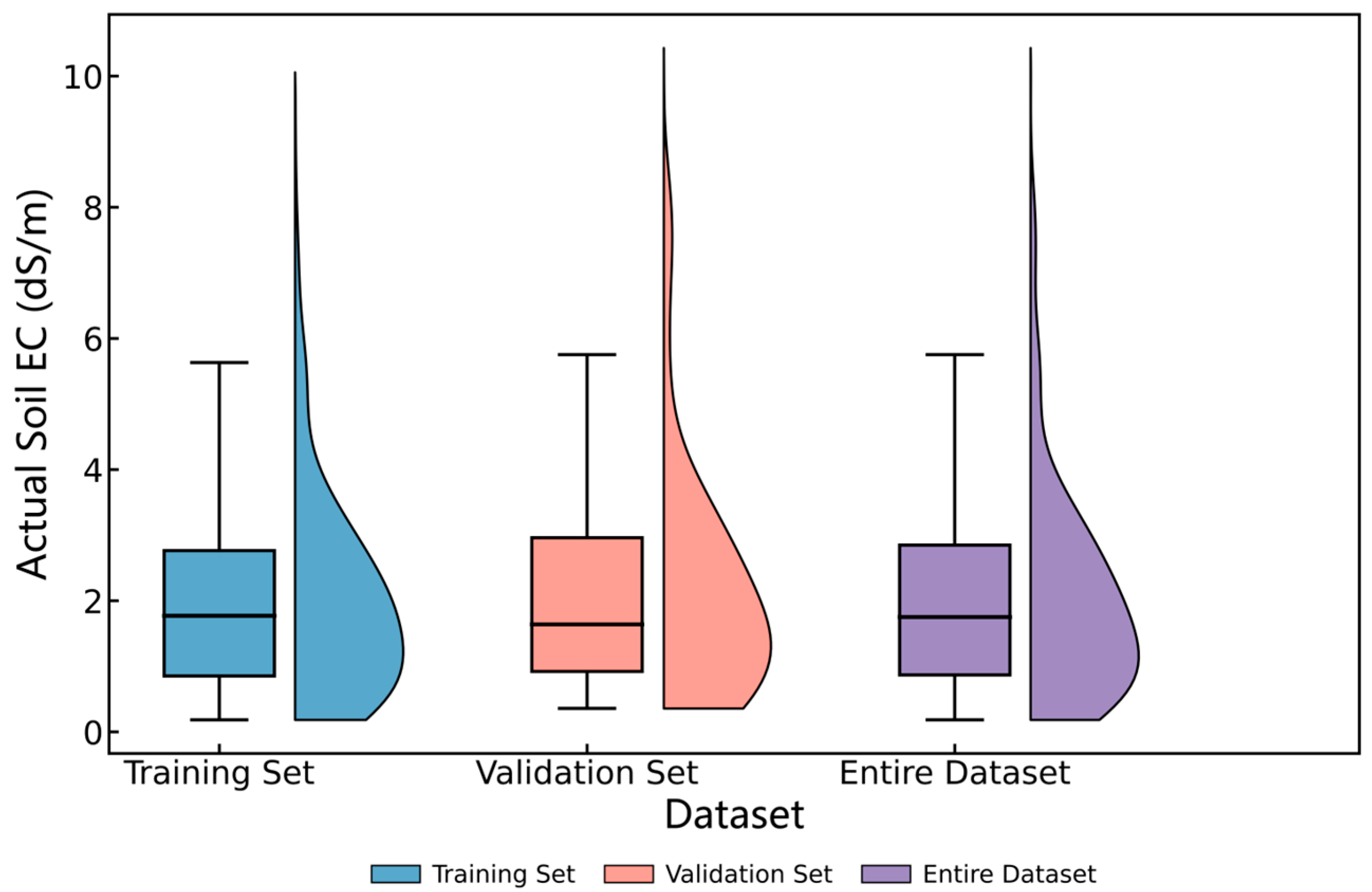
A total of 214 soil samples were collected from the Wei-Ku Oasis and randomly divided into two subsets, with 70% used for model training and 30% for validation. To examine the consistency between the two subsets, violin plots were generated to visualize the distribution of measured soil salinity values across the training set, validation set, and overall dataset (Figure 4). These plots display the distribution density and quartile statistics of each subset. The results indicate that, although minor differences exist, the overall distribution patterns are highly consistent, with no apparent bias between the subsets. This confirms that the data partitioning was representative and appropriate for subsequent modeling and analysis. In this study, the 5-fold CV was performed only on the 70% training subset to evaluate model stability and generalization, while the remaining 30% validation set was reserved for independent testing.

3.2. Selection of Model Input Features

As shown in Figure 5, the Sequential Forward Selection (SFS) method was applied to identify the optimal input features for each model. The feature selection was conducted on the entire dataset to capture the overall statistical characteristics of all samples. For the three CNN-based models, the features were selected based on the minimum validation loss. A lower validation loss was usually associated with higher R2 and lower RMSE and MAE, showing a good balance between accuracy and generalization. For the RF model, since no validation loss was defined, the optimal feature subset was determined using the minimum RMSE.
For the RF model, nine variables were selected: NDWI, SDI, ENDVI, DEM, LST, clay, SI-Albedo, S9, and SI4. The 1 × 1-CNN model retained nine features: SI4, S9, LST, SPAN, NDVI, plan curvature, SI, Albedo, and clay. The 3 × 3-CNN model incorporated fourteen features (NDVI, LST, BI, SI4, S2, S3, DEM, SI-T, SI3, ENDVI, SI-Albedo, EVI, TRI, and SI), reflecting its stronger capacity to capture complex spatial and textural information. In contrast, the MB-CNN model ultimately selected ten variables (NDVI, clay, WTD, TSC, DVI, NDWI, TRI, ENDVI, VV, and SDI), representing an integration of optical, radar, terrain, and hydrological factors.

3.3. Comparison of Model Stability

As shown in Figure 6, among the four models, the MB-CNN exhibited the smallest standard deviations of all evaluation metrics under 5-fold cross-validation, indicating better stability.

3.4. Comparison of Model Accuracy Between Single-Scale CNN and the RF Model

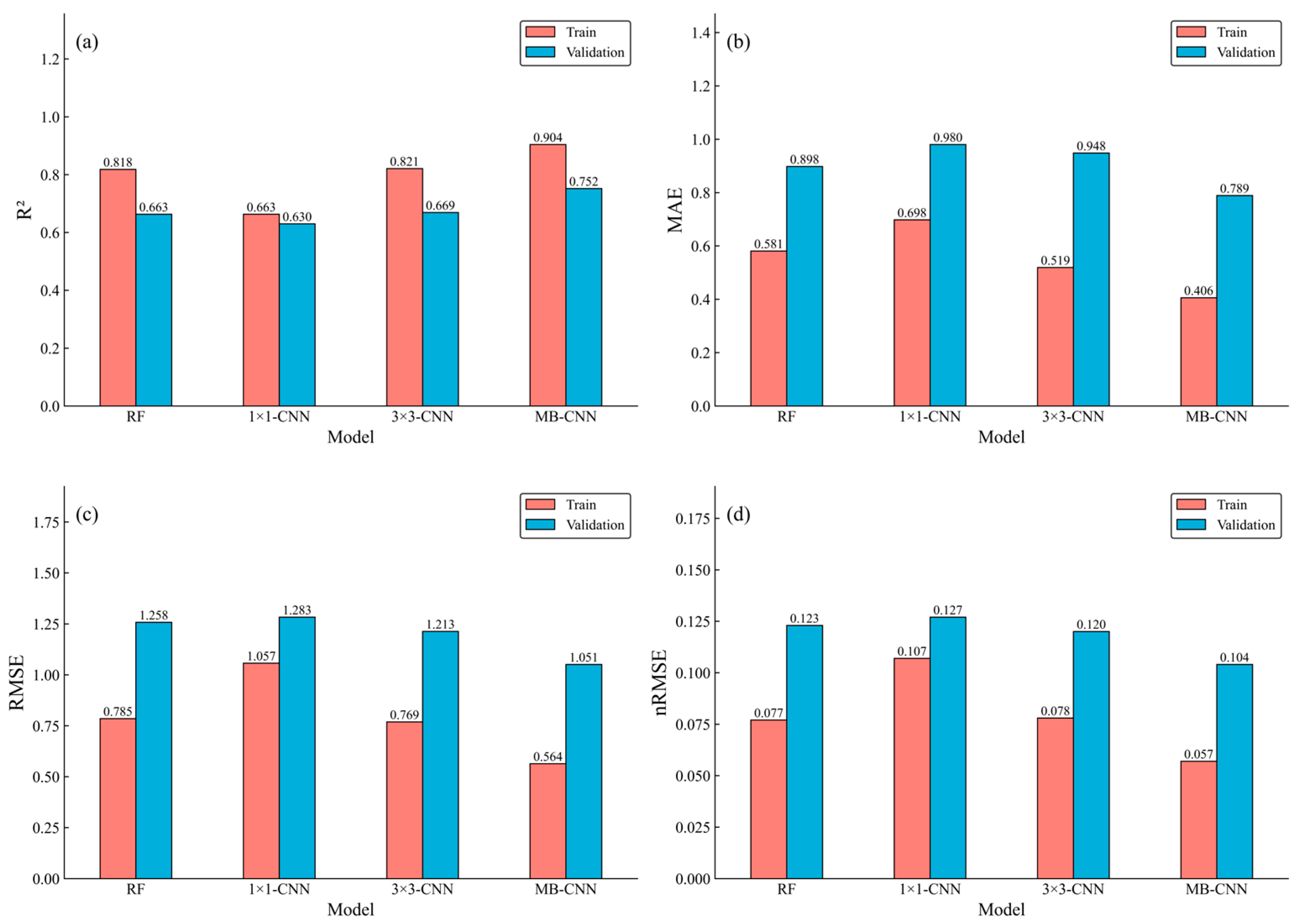
Based on the data analysis and feature selection results, the measured EC data and selected feature subsets were used as inputs to the RF, 1 × 1-CNN, 3 × 3-CNN, and MB-CNN models for soil salinity inversion. Model performance was evaluated on both the training and validation datasets using four statistical metrics: coefficient of determination (R2), mean absolute error (MAE), root mean square error (RMSE), and normalized RMSE (nRMSE). Figure 7 presents grouped bar charts comparing model performance across these evaluation metrics, while Figure 8 illustrates scatter plots of predicted versus measured EC values for both the training and validation sets.
As shown in Figure 8h, a few validation samples fall outside the 95% prediction interval, indicating relatively poor agreement between the observed and predicted EC values for these points. These deviations are mainly attributed to the spatial heterogeneity of soil salinity, which can cause mismatches between the field sampling scale and the satellite pixel scale, particularly in areas with pronounced micro-topographic or irrigation differences. In addition, residual surface moisture may alter spectral and radar responses, leading to larger prediction errors. Despite these few outliers, the MB-CNN model still achieved high overall accuracy in predicting soil salinity.
Overall, the performance of the RF and 1 × 1-CNN models was comparable, with validation R2 values of 0.663 and 0.630 and RMSE values of 1.258 and 1.283, respectively, indicating limited prediction accuracy and generalization capability. In contrast, the 3 × 3-CNN model outperformed both RF and 1 × 1-CNN, achieving a higher validation R2 of 0.669 and a lower RMSE of 1.213, with correspondingly reduced nRMSE and MAE values. The scatter plots further confirm this improvement: the predictions of the 3 × 3-CNN were more tightly clustered around the 1:1 line, suggesting a better fit and more consistent estimation of soil salinity. These results demonstrate that a larger convolution kernel can more effectively capture local spatial features, thereby enhancing both prediction accuracy and model robustness.

3.5. Comparison Between Multi-Scale and Single-Scale CNN Models

Compared with the single-scale convolutional kernel models, the MB-CNN demonstrated superior accuracy and robustness across all evaluation metrics. On the validation dataset, the MB-CNN achieved an R2 of 0.752, substantially higher than that of RF (0.663), 1 × 1-CNN (0.630), and 3 × 3-CNN (0.669). In terms of error metrics, the MB-CNN yielded the lowest MAE (0.789), RMSE (1.051 dS∙m−1), and nRMSE (0.104) among the four models. The scatter plots further reveal that the MB-CNN produced more tightly clustered prediction points and a regression trend closely aligned with the 1:1 line, indicating reduced bias and higher predictive consistency.
Mechanistically, the MB-CNN simultaneously models two receptive fields (1 × 1 and 3 × 3) and fuses their outputs at the feature representation level. The 1 × 1 branch emphasizes intra-pixel and inter-channel relationships, enhancing spectral and feature-level integration, whereas the 3 × 3 branch captures neighborhood spatial context and fine-scale heterogeneity. The complementary synergy between these two branches allows the MB-CNN to mitigate errors and suppress prediction uncertainty, thereby exhibiting enhanced predictive accuracy and robustness for soil salinity inversion in arid regions.
Regarding computational efficiency, the CNN-based models required longer training time than the Random Forest model due to their iterative optimization and multi-epoch learning processes. In addition, the Sequential Forward Selection (SFS) procedure and cross-validation increased the overall computational cost but ensured the robustness and stability of the final results.

3.6. MB-CNN-Based Mapping of Soil EC in the Study Area

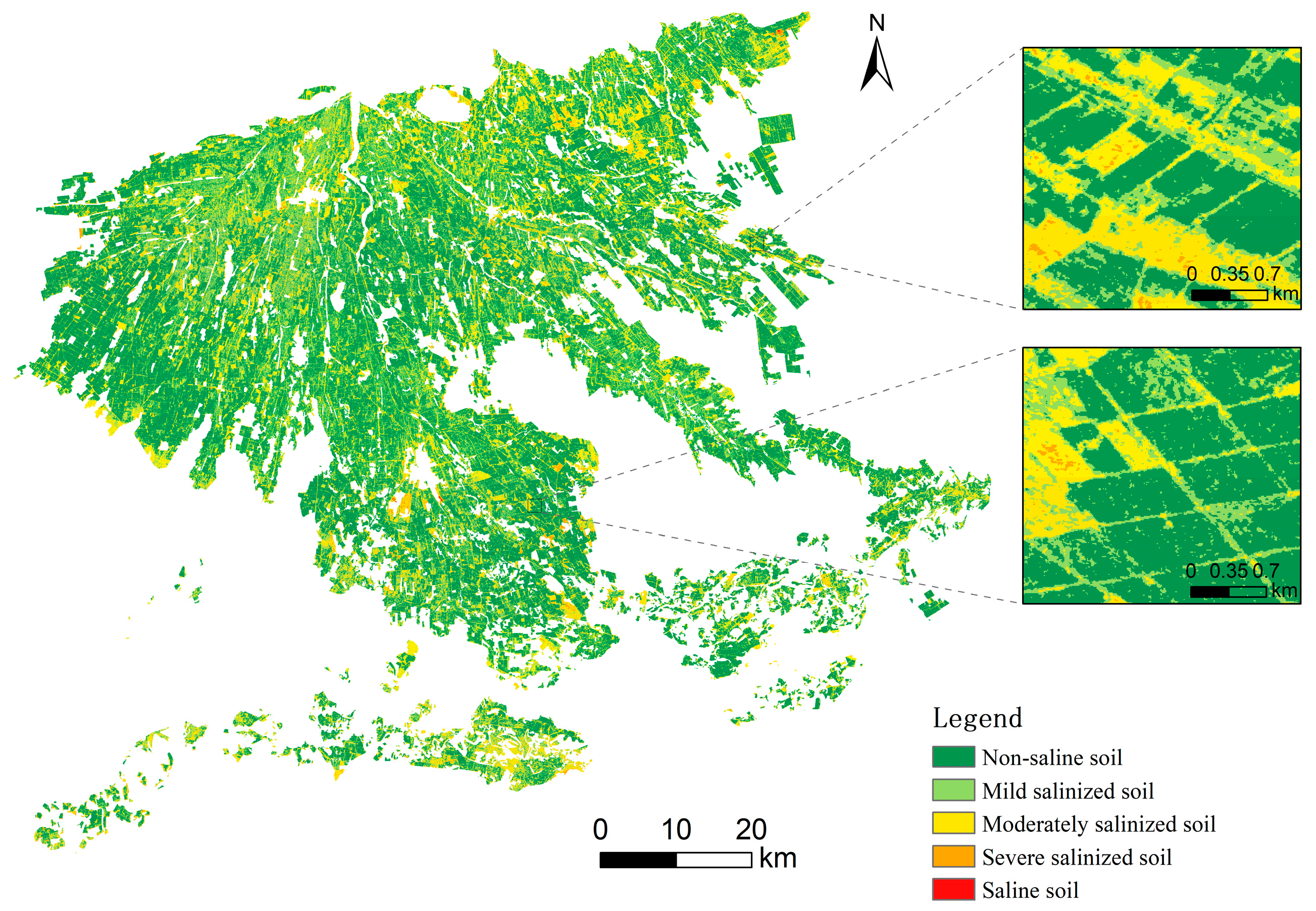
Based on the modeling results described above, the MB-CNN model was applied in combination with remote sensing imagery to generate a spatial inversion of soil electrical conductivity (EC) across the Wei-Ku Oasis. The resulting EC map depicts the continuous spatial pattern of soil salinity throughout the study area. According to the standard classification of soil salinity levels [50], EC values were categorized into five classes: non-saline (0 < EC ≤ 2 dS·m−1), very slightly saline (2 < EC ≤ 4 dS·m−1), slightly saline (4 < EC ≤ 8 dS·m−1), moderately saline (8 < EC ≤ 16 dS·m−1), and strongly saline (EC > 16 dS·m−1). A thematic distribution map was subsequently produced to illustrate the spatial extent and severity of each salinity class across the oasis.
As shown in Figure 9, the overall spatial distribution of soil salinity across the Wei-Ku Oasis exhibits the typical oasis–desert transition pattern characteristic of arid regions, with distinct gradations of salinization intensity. Non-saline soils are primarily concentrated in the western and central irrigated farmlands, whereas slightly and moderately saline soils are mainly distributed within the oasis interior and along river corridors. In contrast, strongly saline soils and solonchaks are predominantly found along the peripheral zones of the oasis. This spatial inversion pattern is consistent with the hydrogeological and topographic differentiation of the Wei-Ku Oasis.
Specifically, areas with lower salinity levels are located on the piedmont alluvial–diluvial fans and within irrigated zones at the southern foothills of the Tianshan Mountains, where gentle relief, good drainage, and effective irrigation leaching prevent salt buildup. Conversely, in the marginal and downstream low-lying areas of the oasis, limited precipitation, high evaporation, and shallow groundwater with strong capillary rise lead to intensive water evaporation and progressive salt buildup in the soil, resulting in severely saline zones.
At the county scale, Xinhe County generally exhibits low salinity levels, dominated by non-saline and slightly saline soils, with only scattered saline patches along the western oasis margins. In contrast, southeastern Kuqa City and southern Shaya County (located within the Tarim River Basin) show more pronounced salinization, primarily characterized by moderately to strongly saline soils, with markedly higher salinity than the northern areas. Overall, the spatial distribution pattern of soil salinity derived from the MB-CNN inversion closely matches the ground survey data, accurately reflecting the root-zone salinity status in the Wei-Ku Oasis and providing a reliable scientific basis for salinization management and irrigation optimization in arid farmlands.

4. Discussion

4.1. Influence of Environmental Variables on Soil Salinity

This study integrated Sentinel-1 and Sentinel-2 data with covariates including topography, climate, soil texture, and groundwater to develop and evaluate four soil salinity inversion models: random forest (RF), 1 × 1-CNN, 3 × 3-CNN, and MB-CNN. The MB-CNN model was employed to generate spatial distribution maps of soil salinity. Through SFS feature selection, optimal input variables were identified for each model. The RF, 1 × 1-CNN, 3 × 3-CNN, and MB-CNN models retained 9, 9, 14, and 10 key features, respectively, covering vegetation, salinity, terrain, radar, and soil-related indices.
Table 4 lists the top 15 features selected by each model. The feature-selection results revealed clear differences among models. The RF model primarily relied on vegetation and surface parameters such as NDWI, SDI, ENDVI, SI-Albedo, and LST, highlighting the importance of vegetation moisture and topographic–thermal factors in soil salinity mapping. The 1 × 1-CNN tended to select transformed spectral indices (e.g., SI4, S9, NDVI, SI, albedo) and several terrain-related variables (slope, plan curvature, TRI), indicating its dependence on high-level spectral abstractions. The 3 × 3-CNN emphasized raw spectral and texture-sensitive features (e.g., BI, S1, S2, S3, SI-T, EVI), reflecting its capability to capture local spatial variations. The MB-CNN combined both high- and low-level information, incorporating optical (NDVI, DVI, ENDVI), radar (VV, SPAN), and environmental variables (clay, WTD, TSC). These patterns suggest that the multi-branch CNN effectively integrates multi-source information across different spatial scales, providing a more comprehensive and physically meaningful representation of soil salinity drivers.
Mechanistically, vegetation indices like NDVI and ENDVI sensitively reflect changes in vegetation cover and moisture status under salinity stress, establishing them as core variables in numerous salinization studies [31,51]. Soil texture indicators such as clay play a critical role in water–salt migration and demonstrate stable performance in salinity prediction [52]. Thermal factors like LST and Albedo reflect surface evapotranspiration and energy balance differences. Related studies indicate that combining these with vegetation indices in arid regions can significantly improve salinity estimation accuracy [53,54]. Topographic factors such as DEM and TRI reveal surface relief, drainage patterns, and salt leaching accumulation, serving as key environmental covariates in salinization mapping [55]. Additionally, multiple salinity indices (SI series) capture salinity signatures at the spectral level, directly enhancing the model’s ability to detect surface salinization. The inclusion of groundwater depth and multiple salinity indices reveals crucial drivers of spatiotemporal salinity migration mechanisms, consistent with existing research on water–salt coupling processes [56]. Meanwhile, VV polarimetric radar data, sensitive to surface moisture content and roughness, effectively enhance salinity identification in areas with low vegetation cover [57]. Thus, despite variations in feature selection across models, they collectively focus on vegetation water content, energy balance, topographic patterns, soil properties, and salinity spectral/radar characteristics. The core environmental factors align with prior research, further validating the reliability and scientific rigor of the model results.

4.2. Influence of Different Models on Soil Salinity Inversion

Previous studies have widely adopted the random forest (RF) model as a baseline for soil salinization mapping, demonstrating its high accuracy and robustness in integrating multi-source covariates. In some cases, RF has even outperformed CNN models [58]. However, its capacity to capture spatial dependencies and neighborhood relationships among pixels remains limited. In contrast, Kazemi Garajeh et al. [59] reported that deep learning models based on CNN achieved higher accuracy in soil salinity inversion, consistent with the findings of this study. The MB-CNN developed herein follows a similar concept to that proposed by Tulczyjew et al. [46] for hyperspectral unmixing, where parallel convolutional branches are employed to extract and fuse multi-type features. This parallel structure significantly enhances predictive accuracy and model stability by combining information from multiple receptive fields. Furthermore, inspired by the work of Hegazi et al. [60] and Yang et al. [61], this study utilized Python in conjunction with the Google Earth Engine API for data preprocessing and model construction, which greatly reduced operational complexity and improved computational efficiency.

4.3. Research Limitations and Future Directions

This study has several limitations. First, climatic and soil conditions in arid regions differ significantly from other areas. The mechanisms governing soil salinity accumulation in humid or temperate zones differ from those in arid zones, limiting the generalizability of this research methodology. Second, this study primarily focuses on salinity monitoring during the crop growing season, without fully considering salinity dynamics during non-growing periods. This may result in an incomplete characterization of the annual salinity process. Third, the multi-branch convolutional structure designed in this study only incorporates 1 × 1 and 3 × 3 convolutional kernels, which may limit the model’s potential for capturing larger-scale spatial patterns. Fourth, the current model validation did not explicitly address spatial autocorrelation, which may lead to potential spatial dependence between training and validation samples. Future studies will adopt spatially stratified or block cross-validation strategies to reduce such effects and improve the robustness of model evaluation.
Future research should extend to diverse climatic zones and ecological types to validate the method’s universality and adaptability. Temporally, integrating year-round or multi-year salinity monitoring data is essential for constructing a comprehensive temporal analysis framework, fully revealing the dynamic evolution of soil salinity. Regarding modeling approaches, incorporating convolutional kernels of other scales (e.g., 5 × 5, 7 × 7), dilated convolutions, and attention mechanisms could enhance the model’s ability to extract complex spatial features, thereby continuously improving the accuracy and application value of soil salinity remote sensing inversion.

4.4. Major Contributions and Practical Implications

From a theoretical perspective, the primary contribution of this study lies in providing a novel approach for the remote sensing modeling of soil properties. By introducing a multi-scale multi-branch convolutional neural network (MB-CNN), which simultaneously utilizes 1 × 1 and 3 × 3 convolutional kernels within the same framework, the model effectively captures salinity-related features across different spatial scales. This approach addresses the limitations of traditional single-scale modeling methods in extracting spatial patterns. This multi-scale feature fusion approach not only enhances the model’s accuracy in salinity inversion for arid regions but also provides a reference methodology for the remote sensing modeling of other soil properties. Furthermore, at the application level, this study enhances the accuracy and stability of salinity distribution mapping by integrating multi-source environmental covariates, providing more reliable data support for managing soil salinization and optimizing irrigation in arid agricultural fields. Thus, the value of this research lies not only in improved model performance but also in establishing a stronger connection between soil property modeling and agricultural practice.

5. Conclusions

This study developed a multi-scale multi-branch convolutional neural network (MB-CNN) model on Python and GEE platforms, incorporating multi-source environmental covariates. It was compared with three soil salinity inversion models—RF, 1 × 1-CNN, and 3 × 3-CNN—to map soil salinity in the Wei-Ku Oasis. The following are this study’s key findings:
The 3 × 3-CNN outperformed both RF and 1 × 1-CNN, indicating that incorporating spatial neighborhood information enhances accuracy in salinity inversion. The MB-CNN demonstrated superior performance compared to both 1 × 1-CNN and 3 × 3-CNN, suggesting that feature layer fusion through multi-scale parallel receptive fields outperforms single-scale convolutional kernels, further improving the accuracy of soil salinity inversion in arid regions.
At the 1 × 1 scale, salinity indices (SI, SI4, S9), vegetation indices (NDVI), and climatic factors (LST) contributed significantly to salinity inversion. At the 3 × 3 scale, terrain factors (DEM, TRI), multi-class salinity indices (SI3, SI-T, S2, S3), and vegetation indices (EVI, ENDVI) play a crucial role in the spatial distribution of salinity. Within the multi-scale integrated MB-CNN model, vegetation indices (NDVI, ENDVI, NDWI, DVI), terrain factors (TRI, TSC), groundwater, and radar characteristics (VV, SDI) collectively exert significant influence, serving as core drivers shaping the spatiotemporal patterns of soil salinity in arid regions.
This study offers novel insights into the remote sensing modeling of soil properties. At the application level, this method substantially enhances the accuracy of soil salinity mapping, providing reliable data support for managing soil salinization and optimizing irrigation in arid agricultural fields.

Author Contributions

Conceptualization, W.D., X.W. and J.S.; methodology, W.D., L.D., S.N. and J.S.; software, W.D. and L.D.; validation, X.W., S.N. and L.D.; formal analysis, X.W., S.N., W.Z. and C.L.; investigation, W.D., X.W., W.Z., Y.H. and S.G.; resources, X.W., S.N., Y.H. and J.S.; data curation, W.D., L.D., W.Z., C.L. and S.G.; writing—original draft preparation, W.D. and L.D.; writing—review and editing, W.D., X.W. and S.N.; visualization, L.D.; supervision, S.N., Y.H. and J.S.; project administration, J.S. and X.W. All authors have read and agreed to the published version of the manuscript.

Funding

This research was funded by the Autonomous Region Key Research and Development Project (2024B03023-2) and the National Key Research and Development Program of China (2021YFD1900801).

Data Availability Statement

The data presented in this study are available on request from the corresponding author.

Acknowledgments

We want to thank the editor and anonymous reviewers for their valuable comments and suggestions to this paper. We also express our sincere gratitude to Zhixin Zhou and Tong Su for their assistance and support during the field sampling and data collection process.

Conflicts of Interest

The authors declare no conflicts of interest.

References

  1. Shokri, N.; Guan, D.; Or, D. Multi-scale soil salinization dynamics from global to pore scales. Rev. Geophys. 2024, 62, e2023RG000804. [Google Scholar] [CrossRef]
  2. Corwin, D.L. Climate change impacts on soil salinity in agricultural areas. Eur. J. Soil Sci. 2020, 71, 265–281. [Google Scholar] [CrossRef]
  3. Zhang, J.; Li, H.; Ma, X. Spatial heterogeneity response of soil salinization in arid oasis agricultural areas. Sci. Rep. 2024, 14, 15160. [Google Scholar]
  4. Hopmans, J.W.; Qureshi, A.S.; Kisekka, I.; Munns, R.; Grattan, S.R.; Rengasamy, P.; Ben-Gal, A.; Assouline, S.; Javaux, M.; Minhas, P.S.; et al. Critical knowledge gaps and research priorities in global soil salinity. In Advances in Agronomy; Sparks, D.L., Ed.; Academic Press: London, UK, 2021; Volume 169, pp. 1–191. [Google Scholar]
  5. Sahbeni, G.; Ngabire, M.; Musyimi, P.K.; Székely, B. Challenges and Opportunities in Remote Sensing for Soil Salinization Mapping and Monitoring: A Review. Remote Sens. 2023, 15, 2540. [Google Scholar] [CrossRef]
  6. Singh, A. Soil salinization management for sustainable development: A review. J. Environ. Manag. 2021, 277, 111383. [Google Scholar] [CrossRef]
  7. Jordan, M.I.; Mitchell, T.M. Machine learning: Trends, perspectives, and prospects. Science 2015, 349, 255–260. [Google Scholar] [CrossRef] [PubMed]
  8. Wang, F.; Han, L.; Liu, L.; Bai, C.; Ao, J.; Hu, H.; Li, R.; Li, X.; Guo, X.; Wei, Y. Advancements and perspective in the quantitative assessment of soil salinity utilizing remote sensing and machine learning algorithms: A review. Remote Sens. 2024, 16, 4812. [Google Scholar] [CrossRef]
  9. Suleymanov, A.; Gabbasova, I.; Komissarov, M.; Suleymanov, R.; Garipov, T.; Tuktarova, I.; Belan, L. Random forest modeling of soil properties in saline semi-arid areas. Agriculture 2023, 13, 976. [Google Scholar] [CrossRef]
  10. Ge, X.; Ding, J.; Teng, D.; Wang, J.; Huo, T.; Jin, X.; Wang, J.; He, B.; Han, L. Updated soil salinity with fine spatial resolution and high accuracy: The synergy of Sentinel-2 MSI, environmental covariates and hybrid machine learning approaches. Catena 2022, 212, 106054. [Google Scholar] [CrossRef]
  11. Zhang, J.; Liu, T.; Feng, W.; Han, L.; Gao, R.; Wang, F.; Ma, S.; Han, D.; Zhang, Z.; Yan, S.; et al. Integrating multi-temporal Sentinel-1/2 vegetation signatures with machine learning for enhanced soil salinity mapping accuracy in coastal irrigation zones: A case study of the Yellow River Delta. Agronomy 2025, 15, 2292. [Google Scholar] [CrossRef]
  12. LeCun, Y.; Bengio, Y.; Hinton, G. Deep learning. Nature 2015, 521, 436–444. [Google Scholar] [CrossRef]
  13. Krizhevsky, A.; Sutskever, I.; Hinton, G.E. ImageNet classification with deep convolutional neural networks. Commun. ACM 2017, 60, 84–90. [Google Scholar] [CrossRef]
  14. Zhu, X.X.; Tuia, D.; Mou, L.; Xia, G.S.; Zhang, L.; Xu, F.; Fraundorfer, F. Deep learning in remote sensing: A comprehensive review and list of resources. IEEE Geosci. Remote Sens. Mag. 2017, 5, 8–36. [Google Scholar] [CrossRef]
  15. Feizizadeh, B.; Garajeh, M.K.; Blaschke, T.; Makki, M. A deep learning convolutional neural network algorithm for detecting saline flow sources and mapping the environmental impacts of the Urmia Lake drought in Iran. Catena 2021, 207, 105585. [Google Scholar] [CrossRef]
  16. Yang, J.; Guo, B.; Zhang, R. The optimal estimation model for soil salinization based on the FOD-CNN spectral index. Remote Sens. 2025, 17, 2357. [Google Scholar] [CrossRef]
  17. Zhang, J.; Wang, X.; Ning, S.; Sheng, J.; Su, T. Spatial heterogeneity response of soil salinization to cotton field expansion in arid regions using deep learning models. Sci. Rep. 2024, 14, 12345. [Google Scholar]
  18. He, Z.; Wang, H.; Yang, S.; Fang, B.; Zhang, Z.; Liu, X. Spatial–temporal differentiation and pattern optimization of landscape ecological security in the Ugan–Kuqa River Oasis. Acta Ecol. Sin. 2019, 39, 5473–5482. [Google Scholar]
  19. Zhang, Q.; Li, L.; Sun, R.; Wang, J.; Chen, Q. Retrieval of soil salinity from Sentinel-1 dual-polarized SAR data based on deep neural network regression. IEEE Geosci. Remote Sens. Lett. 2020, 19, 4006905. [Google Scholar] [CrossRef]
  20. Zhou, T.; Zhu, P.; Yang, R.; Sun, Y.; Sun, M.; Zhang, L.; Li, X. Ecosystem stability in the Ugan–Kuqa River Basin, Xinjiang, China: Investigation of spatial and temporal dynamics and driving forces. Remote Sens. 2024, 16, 4272. [Google Scholar] [CrossRef]
  21. Wang, N.; Chen, S.; Huang, J.; Frappart, F.; Taghizadeh, R.; Zhang, X.; Wigneron, J.-P.; Xue, J.; Xiao, Y.; Peng, J.; et al. Global soil salinity estimation at 10 m using multi-source remote sensing. J. Remote Sens. 2024, 4, 0130. [Google Scholar] [CrossRef]
  22. Wang, J.; Ding, J.; Yu, D.; Teng, D.; He, B.; Chen, X.; Ge, X.; Zhang, Z.; Wang, Y.; Yang, X.; et al. Machine learning-based detection of soil salinity in an arid desert region, Northwest China: A comparison between Landsat-8 OLI and Sentinel-2 MSI. Sci. Total Environ. 2020, 707, 136092. [Google Scholar] [CrossRef]
  23. Zhou, Q.; Zhang, Y.; Liu, Z.; Wang, D.; Chen, H.; Liu, P. Integrating both driving and response environmental variables to enhance soil salinity inversion. Agronomy 2025, 15, 1995. [Google Scholar] [CrossRef]
  24. Jiang, H.; Rusuli, Y.; Amuti, T.; He, Q. Quantitative assessment of soil salinity using multi-source remote sensing data based on the support vector machine and artificial neural network. Int. J. Remote Sens. 2019, 40, 284–306. [Google Scholar] [CrossRef]
  25. Gitelson, A.A.; Kaufman, Y.J.; Merzlyak, M.N. Use of a green channel in remote sensing of global vegetation from EOS-MODIS. Remote Sens. Environ. 1996, 58, 289–298. [Google Scholar] [CrossRef]
  26. Peng, J.; Biswas, A.; Jiang, Q.; Zhao, R.; Hu, J.; Hu, B.; Shi, Z. Estimating soil salinity from remote sensing and terrain data in southern Xinjiang Province, China. Geoderma 2019, 337, 1309–1319. [Google Scholar] [CrossRef]
  27. Major, D.J.; Baret, F.; Guyot, G. A ratio vegetation index adjusted for soil brightness. Int. J. Remote Sens. 1990, 11, 727–740. [Google Scholar] [CrossRef]
  28. Khan, N.M.; Rastoskuev, V.V.; Sato, Y.; Shiozawa, S. Assessment of hydrosaline land degradation by using a simple approach of remote sensing indicators. Agric. Water Manag. 2005, 77, 96–109. [Google Scholar] [CrossRef]
  29. Douaoui, A.E.K.; Nicolas, H.; Walter, C. Detecting salinity hazards within a semiarid context by means of combining soil and remote-sensing data. Geoderma 2006, 134, 217–230. [Google Scholar] [CrossRef]
  30. Bannari, A.; Guedon, A.M.; El-Harti, A.; Cherkaoui, F.Z.; El-Ghmari, A. Characterization of slightly and moderately saline and sodic soils in irrigated agricultural land using simulated data of advanced land imager (EO-1) sensor. Commun. Soil Sci. Plant Anal. 2008, 39, 2795–2811. [Google Scholar] [CrossRef]
  31. Allbed, A.; Kumar, L.; Aldakheel, Y.Y. Assessing soil salinity using soil salinity and vegetation indices derived from IKONOS high-spatial resolution imageries: Applications in a date palm dominated region. Geoderma 2014, 230–231, 1–8. [Google Scholar] [CrossRef]
  32. Liang, S.L. Narrowband to broadband conversions of land surface albedo: I. Algorithms. Remote Sens. Environ. 2001, 76, 213–238. [Google Scholar] [CrossRef]
  33. Liu, J.; Zhang, L.; Dong, T.; Wang, J.; Fan, Y.; Wu, H.; Geng, Q.; Yang, Q.; Zhang, Z. The applicability of remote sensing models of soil salinization based on feature space. Sustainability 2021, 13, 13711. [Google Scholar] [CrossRef]
  34. Nurmemet, I.; Sagan, V.; Ding, J.-L.; Halik, U.; Abliz, A.; Yakup, Z. A WFS-SVM model for soil salinity mapping in Keriya Oasis, northwestern China using polarimetric decomposition and fully PolSAR data. Remote Sens. 2018, 10, 598. [Google Scholar] [CrossRef]
  35. Touzi, R.; Goze, S.; Le Toan, T.; Lopes, A.; Mougin, E. Polarimetric discriminators for SAR images. IEEE Trans. Geosci. Remote Sens. 2002, 30, 973–980. [Google Scholar] [CrossRef]
  36. Zhang, J.; Liu, K.; Wang, M. Downscaling Groundwater Storage Data in China to a 1-km Resolution Using Machine Learning Methods. Remote Sens. 2021, 13, 523. [Google Scholar] [CrossRef]
  37. Saeys, Y.; Inza, I.; Larrañaga, P. A review of feature selection techniques in bioinformatics. Bioinformatics 2007, 23, 2507–2517. [Google Scholar] [CrossRef]
  38. Kohavi, R.; John, G.H. Wrappers for feature subset selection. Artif. Intell. 1997, 97, 273–324. [Google Scholar] [CrossRef]
  39. Chandrashekar, G.; Sahin, F. A survey on feature selection methods. Comput. Electr. Eng. 2014, 40, 16–28. [Google Scholar] [CrossRef]
  40. Mohamed, S.A.; Metwaly, M.M.; Metwalli, M.R.; AbdelRahman, M.A.; Badreldin, N. Integrating active and passive remote sensing data for mapping soil salinity using machine learning and feature selection approaches in arid regions. Remote Sens. 2023, 15, 1751. [Google Scholar] [CrossRef]
  41. Duan, C.; Zhang, Y.; Hu, C.; Chen, H.; Liu, P. Soil salinity inversion by combining multi-temporal Sentinel-2 images near the sampling period in coastal salinized farmland. Front. Environ. Sci. 2025, 13, 1533419. [Google Scholar] [CrossRef]
  42. Taghadosi, M.M.; Hasanlou, M.; Eftekhari, K. Retrieval of soil salinity from Sentinel-2 multispectral imagery. Int. J. Remote Sens. 2019, 40, 510–529. [Google Scholar] [CrossRef]
  43. Liu, R.L.; Jia, K.L.; Li, X.Y.; Zhang, M.L.; Hu, Z.W. Inversion of soil salt content by combining optical and microwave remote sensing in cultivated land. Arid Land Geogr. 2024, 47, 433–444. [Google Scholar]
  44. Song, X.D.; Wu, H.Y.; Ju, B.; Shi, X.; Zhang, G.L. Pedoclimatic zone-based three-dimensional soil organic carbon mapping in China. Geoderma 2020, 363, 114145. [Google Scholar] [CrossRef]
  45. Zhang, L.; Zhang, L.; Du, B. Deep learning for remote sensing data: A technical tutorial on the state of the art. IEEE Geosci. Remote Sens. Mag. 2016, 4, 22–40. [Google Scholar] [CrossRef]
  46. Tulczyjew, Ł.; Kawulok, M.; Longépé, N.; Le Saux, B.; Nalepa, J. A multibranch convolutional neural network for hyperspectral unmixing. IEEE Geosci. Remote Sens. Lett. 2022, 19, 6011105. [Google Scholar] [CrossRef]
  47. Chicco, D.; Warrens, M.J.; Jurman, G. The coefficient of determination R-squared is more informative than SMAPE, MAE, MAPE, MSE and RMSE in regression analysis evaluation. PeerJ Comput. Sci. 2021, 7, e623. [Google Scholar] [CrossRef] [PubMed]
  48. Legates, D.R.; McCabe Jr, G.J. Evaluating the use of “goodness-of-fit” measures in hydrologic and hydroclimatic model validation. Water Resour. Res. 1999, 35, 233–241. [Google Scholar] [CrossRef]
  49. Gorelick, N.; Hancher, M.; Dixon, M.; Ilyushchenko, S.; Thau, D.; Moore, R. Google Earth Engine: Planetary-scale geospatial analysis for everyone. Remote Sens. Environ. 2017, 202, 18–27. [Google Scholar] [CrossRef]
  50. Scudiero, E.; Skaggs, T.H.; Corwin, D.L. Regional-scale soil salinity assessment using Landsat ETM+ canopy reflectance. Remote Sens. Environ. 2015, 169, 335–343. [Google Scholar] [CrossRef]
  51. Metternicht, G.I.; Zinck, J.A. Remote sensing of soil salinity: Potentials and constraints. Remote Sens. Environ. 2003, 85, 1–20. [Google Scholar] [CrossRef]
  52. Ma, W.; Cui, X.; Han, W.; Zhang, H.; Zhang, L. Improved soil salinity estimation in arid regions: Leveraging bare soil periods and environmental factors. iScience 2025, 28, 113020. [Google Scholar] [CrossRef]
  53. Sahbeni, G.; Szatmári, J.; Kovács, F. Soil salinity mapping using Landsat 8 OLI data and regression modeling in the Hungarian Great Plain. SN Appl. Sci. 2021, 3, 587. [Google Scholar] [CrossRef]
  54. Huang, J.; Li, W.; Niu, Z.; Huang, H. Land salinization dynamics based on feature space combinations from Landsat image in Tongyu County, Northeast China. ISPRS Ann. Photogramm. Remote Sens. Spat. Inf. Sci. 2020, 3, 25–32. [Google Scholar] [CrossRef]
  55. Wang, N.; Xue, J.; Peng, J.; Biswas, A.; He, Y.; Shi, Z. Integrating remote sensing and landscape characteristics to estimate soil salinity using machine learning methods: A case study from Southern Xinjiang, China. Remote Sens. 2020, 12, 4118. [Google Scholar] [CrossRef]
  56. Wei, Y.; Wang, F.; Hong, B.; Yang, S. Revealing spatial variability of groundwater level in typical ecosystems of the Tarim Basin through ensemble algorithms and limited observations. J. Hydrol. 2023, 620, 129399. [Google Scholar] [CrossRef]
  57. Baghdadi, N.; Zribi, M.; Loumagne, C.; Ansart, P.; El Hajj, M. Estimating soil moisture with C-band radar data: Application to ERS-SAR data over wheat fields. Remote Sens. Environ. 2016, 96, 443–451. [Google Scholar]
  58. Yan, Y.; Kayem, K.; Hao, Y.; Shi, Z.; Zhang, C.; Peng, J.; Liu, W.; Zuo, Q.; Ji, W.; Li, B. Mapping the levels of soil salination and alkalization by integrating machine learning methods and soil-forming factors. Remote Sens. 2022, 14, 3020. [Google Scholar] [CrossRef]
  59. Garajeh, M.K.; Malakyar, F.; Weng, Q.; Feizizadeh, B.; Blaschke, T.; Lakes, T. An automated deep learning convolutional neural network algorithm applied for soil salinity distribution mapping in Lake Urmia, Iran. Sci. Total Environ. 2021, 778, 146253. [Google Scholar] [CrossRef]
  60. Hegazi, E.H.; Samak, A.A.; Yang, L.; Huang, R.; Huang, J. Prediction of soil moisture content from Sentinel-2 images using convolutional neural network (CNN). Agronomy 2023, 13, 656. [Google Scholar] [CrossRef]
  61. Yang, G.; Wang, J.; Qi, Z. Maize classification in arid regions via spatiotemporal feature optimization and multi-source remote sensing integration. Agronomy 2025, 15, 1667. [Google Scholar] [CrossRef]
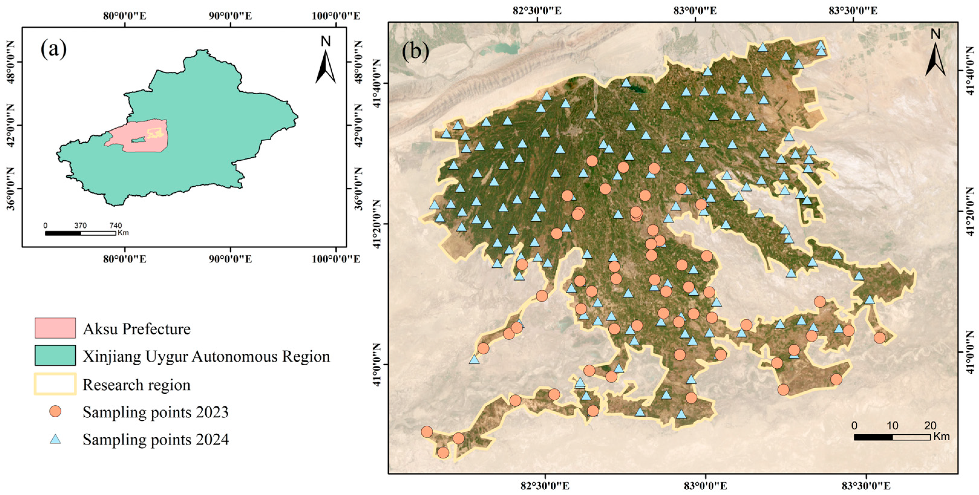
Figure 1. (a) Location of study area. Administrative boundaries in panel (a) are derived from the Standard Map Service (Tianditu), Ministry of Natural Resources of China (Map Review Number: GS(2024)0605). (b) Distribution of cropland sampling sites in Wei-Ku Oasis (sampling in 2023 and 2024).
Agronomy 15 02534 g001
Figure 2. Schematic diagram of a single-scale convolutional kernel CNN model.
Agronomy 15 02534 g002
Figure 3. Structure of the multi-branch convolutional neural network (MB-CNN).
Agronomy 15 02534 g003
Figure 4. Violin plots of measured soil salinity for the training set, validation set, and overall dataset.
Agronomy 15 02534 g004
Figure 5. Feature selection results of the RF, 1 × 1-CNN, 3 × 3-CNN, and MB-CNN models.
Agronomy 15 02534 g005
Figure 6. Comparison of model performance and stability based on 5-fold cross-validation (Mean ± Std).
Agronomy 15 02534 g006
Figure 7. Model evaluation results for RF, 1 × 1-CNN, 3 × 3-CNN, and MB-CNN based on four performance metrics: (a) coefficient of determination (R2), (b) mean absolute error (MAE), (c) root mean square error (RMSE), and (d) normalized root mean square error (nRMSE).
Agronomy 15 02534 g007
Figure 8. Scatter plots of measured versus predicted EC values derived from the inversion models (RF (a,b), 1 × 1-CNN (c,d), 3 × 3-CNN (e,f), and MB-CNN (g,h)).
Agronomy 15 02534 g008aAgronomy 15 02534 g008b
Figure 9. Spatial distribution map of farmland soil salinity derived from the MB-CNN model.
Agronomy 15 02534 g009
Table 1. Thirty covariates with their feature types, descriptions, and formulas.
Feature TypesDescriptionFormulaReference
Vegetation indicesNormalized differential vegetation index N D V I = ( N I R R ) / ( N I R + R ) [22]
Enhanced vegetation index E V I = 2.5   ×   ( NIR R ) / ( N I R + 6 R 7.5 B + 1 ) [23]
Normalized difference water index N D W I = ( N I R S W I R 1 ) / ( N I R + S W I R 1 ) [24]
Soil-adjusted vegetation index S A V I = ( 1 + L ) × ( N I R R ) / ( N I R + R + L ) [25]
Enhanced normalized differential vegetation index E N D V I = ( N I R + S W I R 1 R ) × ( N I R + S W I R 2 + R ) [22]
Differential vegetation index D V I = N I R R [26]
Salinity indicesNormalized difference salinity index N D S I = ( R N I R ) / ( R + N I R ) [27]
Salinity index S I = G × R [21]
Salinity index 1 S I 1 = G + R [28]
Salinity index 2 S I 2 = N I R 2 + G 2 + R 2 [28]
Salinity index 3 S I 3 = G 2 + R 2 [28]
Salinity index 4 S I 4 = S W I R 1 / N I R [29]
Salinity index I S 1 = B / R [28]
Salinity index II S 2 = ( B R ) / ( B + R ) [28]
Salinity index III S 3 = G × R / B [28]
Salinity index V S 5 = B × R / G [28]
Salinity index VI S 6 = R × N I R / G [28]
Salinity index VII S 7 = ( S W I R 1 S W I R 2 ) / ( S W I R 1 + S W I R 2 ) [30]
Salinity index VIII S 8 = ( G + R ) / 2 [29]
Salinity index IX S 9 = ( G + R + N I R ) / 2 [29]
Salinity index S I T = R / N I R × 100 [31]
Soil indicesBrightness index B I = G 2 + R 2 [28]
Albedo0.36B + 0.13R + 0.37NIR + 0.09SWIR1 + 0.07SWIR2 − 0.002[32]
Feature spaceSI-Albedo S I A l b e d o = A l b e d o 2 + ( B × R ) 2 [33]
Original backscatter featureNormalized backscatter coefficient γ v v 0 , γ v h 0 -
Radar indexRadar vegetation index R V I = γ v v 0 / ( γ v v 0 + γ v h 0 ) [34]
Square difference index S D I = ( γ v v 0 2 γ v h 0 2 ) / ( γ v v 0 2 + γ v h 0 2 ) [19]
Ratio of backscatter coefficient R a t i o = γ v v 0 / γ v h 0 [19]
Total scattering power S P A N = ( γ v v 0 2 + γ v h 0 2 ) [35]
Normal difference index N D I = γ v v 0 γ v h 0 [19]
Table 2. Geospatial covariates with their spatial resolution and data source.
Feature TypeCovariateSpatial ResolutionData Source
Terrain dataDEM30 mNASA JPL, SRTM V3 (SRTM Plus)
Digital Elevation Model
Slope30 m
Aspect30 m
Plan curvature30 m
Profile curvature30 m
Terrain ruggedness index (TRI)30 m
Topographic surface convexity (TSC)30 m
Climate dataLand Surface temperature (LST)1000 mMOD11A1 Version 6.1
(MODIS, NASA LP DAAC)
Evapotranspiration (ET)500 mMOD16A2 Version 6.1
(MODIS, NASA LP DAAC)
Soil texture dataClay250 mSoilGrids (ISRIC–World Soil Information)
Sand250 m
Silt250 m
GroundwaterGroundwater table depth (WTD)1000 m[36]
Table 3. Hyperparameter configuration and network settings of the CNN-based models.
CategoryParameterSetting
Model structureConvolutional layersTwo layers per branch (32 filters each)
Kernel size1 × 1 (1 × 1-CNN), 3 × 3 (3 × 3-CNN),
dual 1 × 1 & 3 × 3 (MB-CNN)
Pooling layerAdaptive average pooling
Fully connected layers32 → 1
Training configurationLoss functionSmooth L1 loss
OptimizerAdamW
Learning rate0.01
Weight decay1 × 10−4
Batch size16
Epochs200 (with early stopping, patience = 10)
ImplementationFrameworkPyTorch 2.4.1
Table 4. Top 15 input variables identified through SFS feature selection for each model.
RankRF1 × 1-CNN3 × 3-CNNMB-CNN
1NDWISI4NDVINDVI
2SDIS9LSTClay
3ENDVILSTBIWTD
4DEMSPANSI4TSC
5LSTNDVIS2DVI
6ClayPlan curvatureS3NDWI
7SI-AlbedoSIDEMTRI
8S9AlbedoSI-TENDVI
9SI4ClaySI3VV
10RVIDEMENDVISDI
11SI2SlopeSI-AlbedoAlbedo
12S3DVIEVISI2
13S2BITRISI-T
14S1VHSISlope
15BITRIS1SPAN
Disclaimer/Publisher’s Note: The statements, opinions and data contained in all publications are solely those of the individual author(s) and contributor(s) and not of MDPI and/or the editor(s). MDPI and/or the editor(s) disclaim responsibility for any injury to people or property resulting from any ideas, methods, instructions or products referred to in the content.