Article

Spectral Index Optimization and Machine Learning for Hyperspectral Inversion of Maize Nitrogen Content

1
College of Water Resources and Hydropower Engineering, Gansu Agricultural University, Lanzhou 730070, China
2
Xinjiang Research Institute of Agriculture in Arid Areas, Urumqi 830091, China
3
College of Water Resources and Architectural Engineering, Northwest A & F University, Yangling 712100, China
*
Author to whom correspondence should be addressed.
Agronomy 2025, 15(11), 2485; https://doi.org/10.3390/agronomy15112485
Submission received: 13 September 2025 / Revised: 13 October 2025 / Accepted: 23 October 2025 / Published: 26 October 2025

Abstract

Hyperspectral remote sensing provides a powerful tool for crop nutrient monitoring and precision fertilization, yet its application is hindered by high-dimensional redundancy and inter-band collinearity. This study aimed to improve maize nitrogen estimation by constructing three types of two-dimensional full-band spectral indices—Difference Index (DI), Simple Ratio Index (SRI), and Normalized Difference Index (NDI)—combined with spectral preprocessing methods (raw spectra (RAW), first-order derivative (FD), and second-order derivative (SD)). To optimize feature selection, three strategies were evaluated: Grey Relational Analysis (GRA), Pearson Correlation Coefficient (PCC), and Variable Importance in Projection (VIP). These indices were then integrated into machine learning models, including Backpropagation Neural Network (BP), Random Forest (RF), and Support Vector Regression (SVR). Results revealed that spectral index optimization substantially enhanced model performance. NDI consistently demonstrated robustness, achieving the highest grey relational degree (0.9077) under second-derivative preprocessing and improving BP model predictions. PCC-selected features showed superior adaptability in the RF model, yielding the highest test accuracy under raw spectral input (R2 = 0.769, RMSE = 0.0018). VIP proved most effective for SVR, with the optimal SD–VIP–SVR combination attaining the best predictive performance (test R2 = 0.7593, RMSE = 0.0024). Compared with full-spectrum input, spectral index optimization effectively reduced collinearity and overfitting, improving both reliability and generalization. Spectral index optimization significantly improved inversion accuracy. Among the tested pipelines, RAW-PCC-RF demonstrated robust stability across datasets, while SD-VIP-SVR achieved the highest overall validation accuracy (R2 = 0.7593, RMSE = 0.0024). These results highlight the complementary roles of stability and accuracy in defining the optimal pipeline for maize nitrogen inversion. This study highlights the pivotal role of spectral index optimization in hyperspectral inversion of maize nitrogen content. The proposed framework provides a reliable methodological basis for non-destructive nitrogen monitoring, with broad implications for precision agriculture and sustainable nutrient management.

1. Introduction

In the context of sustainable modern agriculture, achieving precise crop nutrient monitoring and scientific fertilization management has become a critical pathway to enhancing agricultural efficiency, ensuring food security, and reducing environmental pollution [1]. Nitrogen is widely recognized as the most essential macronutrient for maize growth, acting as a structural component of proteins, chlorophyll, and nucleic acids [2], and directly regulating photosynthesis, biomass accumulation, and yield formation. It directly influences photosynthetic efficiency, dry matter accumulation, and final yield formation through participation in key enzymatic reactions, such as photophosphorylation and nitrate assimilation, as well as the regulation of plant hormone synthesis and metabolism [3]. Maize exhibits high sensitivity to nitrogen supply, and excessive nitrogen application not only leads to resource waste but also contributes to groundwater nitrate pollution and increased greenhouse gas emissions [4]. Therefore, developing non-destructive, efficient, and accurate monitoring approaches for maize nitrogen content is urgently needed to advance green agriculture [5,6].
Traditional destructive sampling methods for biochemical content inversion are time-consuming, labor-intensive [7], and limited in spatial coverage, making them unsuitable for real-time, large-scale field monitoring. Conventional remote sensing technologies, due to their low spectral resolution, fail to capture fine spectral features within narrow wavelength ranges, resulting in limited accuracy for biochemical parameter inversion [8]. Previous studies have confirmed that maize leaves exhibit distinct absorption peaks in the blue (approximately 430 nm) and red (approximately 660 nm) spectral regions, high reflectance in the green band (approximately 550 nm) [9], and elevated reflectance in the near-infrared region (700–1300 nm) influenced by internal leaf structure [10]. Specifically, the 690–700 nm band is highly sensitive to stress-induced chlorophyll content changes, and the 760–790 nm range effectively reflects plant water stress [11], and the 730 nm and 960 nm bands are closely associated with plant water absorption bands [12]. Hyperspectral technology, with its hundreds to thousands of continuous narrow bands, can sensitively capture subtle spectral differences in crop leaves across the visible to near-infrared spectrum, establishing a strong correlation between spectral signals and biochemical content [13], thus providing reliable technical support for accurate maize nitrogen content inversion [14,15,16].
However, hyperspectral data suffer from high information volume, significant band redundancy, and strong collinearity among variables, which constrain their application in high-precision inversion of crop physiological parameters. Li et al. (2023) found that redundant information and high collinearity in hyperspectral data limit the effectiveness and accuracy of model simulations [17]. To address this, researchers commonly employ feature selection or extraction techniques to reduce spectral data dimensionality, extracting the most representative spectral features for target variables. Zhang et al. (2019) noted that while short-wave infrared (SWIR) bands can enhance the accuracy of water and nitrogen content inversion in high-throughput remote sensing phenotyping, selecting a limited set of high-quality band combinations through appropriate dimensionality reduction significantly improves model stability and efficiency [18,19]. Among various dimensionality reduction methods, spectral indices are widely used due to their dual functionality in feature construction and selection. For instance, classic vegetation indices like NDVI and EVI enhance spectral contrast relationships through physical or mathematical formulations [20], extracting highly sensitive feature combinations in subsequent selections. Compared to conventional feature algorithms, spectral indices offer advantages such as multi-band synergy, high information utilization, and clear physical significance [21,22].
Spectral indices have evolved rapidly. Although classic indices are widely applied in crop monitoring, their reliance on fixed sensitive bands makes them susceptible to background interference under varying environmental conditions, limiting model generalization. With advancing research, spectral index construction has moved beyond traditional optical property constraints, adopting band-by-band combinatorial approaches. Chen et al. demonstrated that such methods can significantly improve accuracy under specific regional and sample conditions but often face the “curse of dimensionality” [23], creating a trade-off between computational efficiency and result stability. Consequently, selecting optimal band combinations through scientific methods to achieve spectral index optimization has become a core component in enhancing the predictive capability for crop physiological parameters. Most current studies rely solely on the Pearson Correlation Coefficient (PCC) for spectral index selection. While PCC is simple and effective for measuring linear correlations, it fails to capture nonlinear relationships between spectral indices and nitrogen content [24], often resulting in insufficiently representative selected indices. Alternative feature selection methods, such as Grey Relational Analysis (GRA) and Variable Importance in Projection (VIP), have not been widely applied in spectral index optimization [25]. Additionally, neglecting the compatibility between spectral index optimization methods and modeling algorithms [26], as well as failing to tailor index selection strategies to the characteristics of different machine learning models, limits the predictive potential of spectral indices, ultimately affecting model inversion accuracy and generalization [27,28]. To ensure consistent evaluation, we also predefined a single selection rule for determining the overall optimal pipeline: the configuration achieving the highest R2 on the independent validation set, with RMSE used as the secondary criterion. The detailed implementation is described in the Methods section.
To address these gaps, this study proposes a comprehensive framework for maize nitrogen estimation that integrates full-band index construction, preprocessing methods (RAW, FD, SD), and multiple feature selection strategies (GRA, PCC, VIP). The optimized indices are then coupled with three representative machine learning models—Backpropagation Neural Network (BP), Random Forest (RF), and Support Vector Regression (SVR)—to evaluate their predictive performance and stability. Specifically, we aim to: (i) compare the adaptability of different indices and selection methods, (ii) identify the optimal selection–modeling combination for nitrogen inversion, and (iii) provide methodological insights for non-destructive nitrogen monitoring to support precision agriculture [29].

2. Materials and Methods

2.1. Study Site and Experimental Design

The study was conducted at the Dryland Agriculture Experimental Station in Yuzhong County (104°09′ E, 35°56′ N; altitude 1749 m, Figure 1), Gansu province, China, which is situated in a typical semi-arid climatic zone. The site has an average annual evaporation of 1450 mm, mean annual precipitation of 327 mm (mainly concentrated from July to September), mean annual temperature of 7.6 °C, accumulated temperature ≥0 °C is 3244 °C, accumulated temperature ≥10 °C is 2479 °C, and annual sunshine duration ranging from 1626 to 2666 h.
A field experiment was conducted to investigate the effects of varying plant densities (42,000, 63,000, and 84,000 plants ha−1) and nitrogen application rates (0, 80, 160, and 240 kg N ha−1) on maize growth. Plant densities were achieved by adjusting row spacing, combined with four nitrogen levels, resulting in 12 treatment combinations. Each treatment was replicated three times, yielding a total of 36 plots. A 2-m buffer zone was established around the experimental area, and 1-m isolation strips between adjacent plots. Maize was sown on 25 April 2024 and harvested on 27 September 2024. Irrigation was scheduled based on reference crop evapotranspiration (ET0), while other management practices followed local recommendations.

2.2. Data Collection

Hyperspectral data were collected on 5 July, 11 July, 16 August, and 22 August 2024. Canopy spectral reflectance of maize was measured using a FieldSpec 4 spectroradiometer (Analytical Spectral Devices, Inc., Boulder, CO, USA) covering the 350–2500 nm range. The sampling interval was 1.4 nm for 350–1000 nm and 2 nm for 1001–2500 nm. The spectral resolution was 3 nm at 700 nm, 10 nm at 1400 nm, and 10 nm at 2100 nm [30]. The instrument automatically interpolated the sampled data to 1 nm intervals for output. The fiber optic cable length was 1.5 m, with a field-of-view angle of 25°. Measurements were taken under clear, windless conditions between 11:00 and 14:00, ensuring the fiber optic probe was oriented vertically downward and positioned approximately 1 m above the canopy top. For each plot, three representative quadrats were selected to reflect the plot’s growth status. Ten spectral curves were recorded per quadrat, and the average was used as the spectral reflectance for that quadrat [31], resulting in a total of 144 datasets. A standard whiteboard calibration was performed prior to each sample measurement. Destructive sampling was conducted synchronously within the hyperspectral measurement quadrats to determine maize canopy nitrogen content. Data processing and analysis were conducted using ViewSpecPro Version6.2 (ASD Inc., Boulder, CO, USA) for spectral data inspection and calibration, and MATLAB R2023b (MathWorks, Natick, MA, USA) for spectral index construction, feature selection, and model implementation.

2.3. Spectral Data Preprocessing

Raw spectra comprehensively record the absorption and scattering information generated by the interaction between samples and light. However, they inevitably include interferences such as instrumental background noise and baseline drift, which introduce uncertainty into subsequent analyses. To minimize errors and enhance the signal-to-noise ratio of spectral data, preprocessing of the raw spectra is essential. Existing spectral preprocessing techniques are diverse and can be categorized into four main types based on their characteristics: baseline correction [32], scatter correction [33], smoothing, and proportional scaling (Table 1) [34]. The final preprocessing method was determined according to the correlation between spectral information features and nitrogen content, with raw spectra (RAW), first-order derivative (FD), and second-order derivative (SD) were selected as the three preprocessing approaches.

2.4. Spectral Index Construction and Selection Methods

To fully exploit the spectral features in hyperspectral data that are most sensitive to variations in maize nitrogen content, this study selected three types of two-dimensional spectral indices based on a full-band combination strategy: Normalized Difference Index (NDI), Simple Ratio Index (SRI), and Difference Index (DI) [37,38,39,40,41,42]. The specific formulas are given in Equations (1)–(3). Subsequently, three representative feature optimization methods were employed for feature selection and comparative analysis, thereby yielding effective input variables for subsequent modeling.
N D I i , j = R i R j R i + R j
D I i , j = R i R j
S R I i , j = R i R j
where Ri and Rj represent the reflectance at wavelengths i and j, respectively.
Hyperspectral data exhibit high dimensionality and strong inter-band correlations. Direct use in modeling can easily lead to overfitting and compromise model stability; therefore, feature optimization is essential. This study employed three methods—Grey Relational Analysis (GRA), Pearson Correlation Coefficient (PCC), and Variable Importance in Projection (VIP)—to screen the constructed spectral indices, identifying sensitive band features that are highly correlated with maize nitrogen content.
(1) Grey Relational Analysis (GRA)
Grey Relational Analysis (GRA), based on grey system theory, measures the degree of association between variables by comparing the geometric similarity between the reference sequence and comparison sequences. It is particularly suitable for analyzing small samples and non-normally distributed data [43]. The calculation formula is:
ξ i ( k ) = m i n i m i n k X 0 ( k ) X i ( k ) + ρ m a x i m i n k X 0 ( k ) X i ( k ) X 0 ( k ) X i ( k ) + ρ m a x i m i n k X 0 ( k ) X i ( k )
where ξi(k) represents the correlation coefficient of sequence Xi at time k, X0(k) is the reference sequence, and ρ is the resolution coefficient (typically set to 0.5). The mean value of the correlation coefficients is the grey relational degree, which is used to measure the correlation between the spectral index and nitrogen content.
(2) Pearson Correlation Coefficient (PCC)
The Pearson Correlation Coefficient (PCC) is used to measure the linear correlation between spectral indices and nitrogen content, with larger absolute values indicating stronger correlations [44]. The calculation formula is:
r = i = 1 n X i X ¯ Y i Y ¯ i = 1 n X i X ¯ 2 i = 1 n Y i Y ¯ 2
where r is the Pearson correlation coefficient, ranging from [−1, 1], with absolute values closer to 1 indicating stronger correlation; Xi and Yi represent the values of the two variables for the i observation sample; X ¯ and Y ¯ are the means of the two variables; and n is the number of samples.
(3) Variable Importance in Projection (VIP)
The Variable Importance in Projection (VIP) score, based on the Partial Least Squares Regression (PLSR) model, is used to comprehensively evaluate the contribution of each variable to model interpretation and prediction. It performs exceptionally well in handling multicollinearity and high-dimensional feature data [45]. The calculation formula is:
V I P j = p a = 1 A S S Y a w j a 2 w a 2 a = 1 A S S Y a
where VIPj represents the VIP value of the j-th variable, p is the total number of independent variables, wja denotes the weight of variable j in the a-th latent variable, ‖wa‖ is the Euclidean norm of the weight vector, and SSYa is the sum of squares explained by latent variable a for the dependent variable. Generally, a variable is considered an important feature when VIP > 1.

2.5. Model Construction

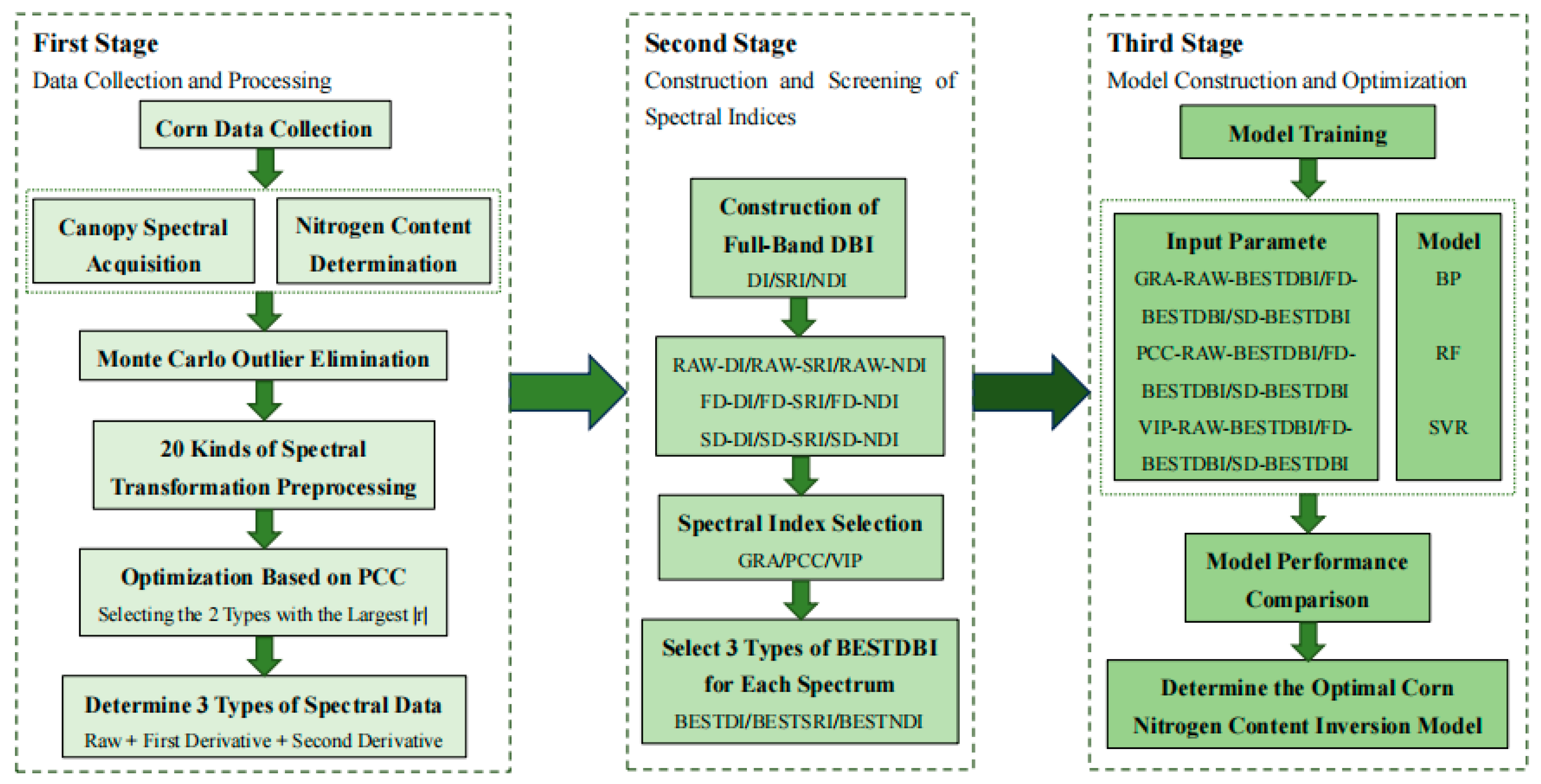
To comprehensively evaluate the adaptability and predictive capability of different feature selection strategies in spectral inversion modeling, the top-ranked spectral indices (based on scores) were selected using GRA, PCC, and VIP as input variables, with maize plant nitrogen content serving as the dependent variable. Three typical regression models were constructed: Backpropagation Neural Network [46] (BP), Random Forest [47] (RF), and Support Vector Regression (SVR). Each model offers distinct advantages, making them suitable for nonlinear regression, high-dimensional multivariate inputs, and small-sample modeling scenarios, with strong generalization ability and robustness.The methodological workflow of the entire process (including spectral index construction, feature selection, and model construction) is illustrated in Figure 2, which is the methodological workflow diagram for this study.
During the model performance evaluation phase, the R2 (Formula (6)) was used to measure the model’s ability to explain the variance in PNC, where a value closer to 1 signifies a better model fit. The (RMSE, Formula (7)) quantified the average magnitude of the deviation between predicted and observed values, with lower values indicating higher prediction accuracy. We predefined the optimal pipeline as the configuration achieving the highest R2 on the independent validation set, with RMSE as a secondary criterion. In addition, to ensure practical interpretability, we also report robust pipelines that show stable performance across preprocessing scenarios and datasets.
R 2 = i = 1 n ( y ^ i y ¯ ) i = 1 n ( y i y ¯ )
R M S E = i = 1 n ( y ^ i y i ) 2 n

3. Results

3.1. Spectral Preprocessing

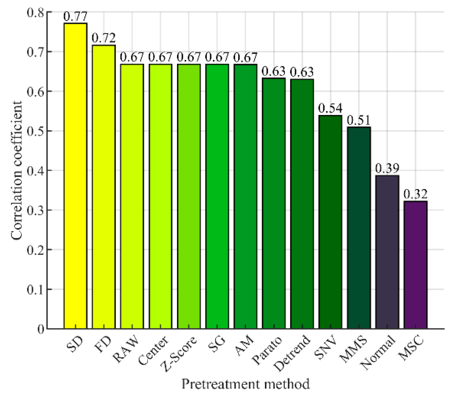
The maximum correlation coefficients between preprocessing methods and nitrogen content are shown in Figure 3. FD and SD were selected as superior methods, with RAW as the control. Figure 4 shows the spectra. The RAW curve (Figure 4a) captures canopy reflectance and nitrogen-related features, especially in the red edge (700–750 nm) and NIR (800–1000 nm), but is affected by baseline drift and noise.
FD (Figure 4b) emphasizes slope changes, improving the discrimination of absorption boundaries, particularly between red and red edge (550–750 nm). SD (Figure 4c) highlights curvature and inflection points, performing well under noisy conditions and overlapping peaks, especially in the NIR and SWIR regions (1350–1450 nm). In summary, RAW preserves full reflectance, FD enhances gradients, and SD extracts subtle features. All three datasets were used in subsequent index construction and modeling. As observed in the figures, the RAW spectrum retains complete reflectance information, making it suitable for constructing and interpreting traditional spectral indices. The FD spectrum enhances gradient information, facilitating the extraction of change boundaries, while the SD spectrum excels in amplifying subtle features and mitigating overlapping interference. To improve model adaptability and feature extraction capability, subsequent analyses in this study will involve constructing and screening spectral indices, as well as modeling, using all three datasets.

3.2. Results of Spectral Index Construction and Selection

The maximum correlation values between the spectral indices extracted from Figure 5, Figure 6 and Figure 7 (a–i) and nitrogen content, along with their corresponding wavelength positions, are presented in Table 2. All three feature selection methods identified highly correlated bands but differed in performance. With GRA, NDI achieved the highest grey relational degree: ξ_max = 0.8947 (RAW, 700–1801 nm), 0.9037 (FD, 679–1639 nm), and 0.9077 (SD, 547–551 nm). PCC favored SRI, with r_max = 0.8313 (547–551 nm), highlighting sensitivity to red edge and visible regions. VIP selected bands mainly in the red edge and NIR (1595–1596 nm, 1153–721 nm, 1778–2398 nm), enhancing model explanatory power. Overall, GRA emphasized NDI, PCC highlighted SRI, and VIP identified red edge/NIR synergy, confirming the red edge as the key region for nitrogen retrieval.

3.3. Model Prediction Results and Analysis

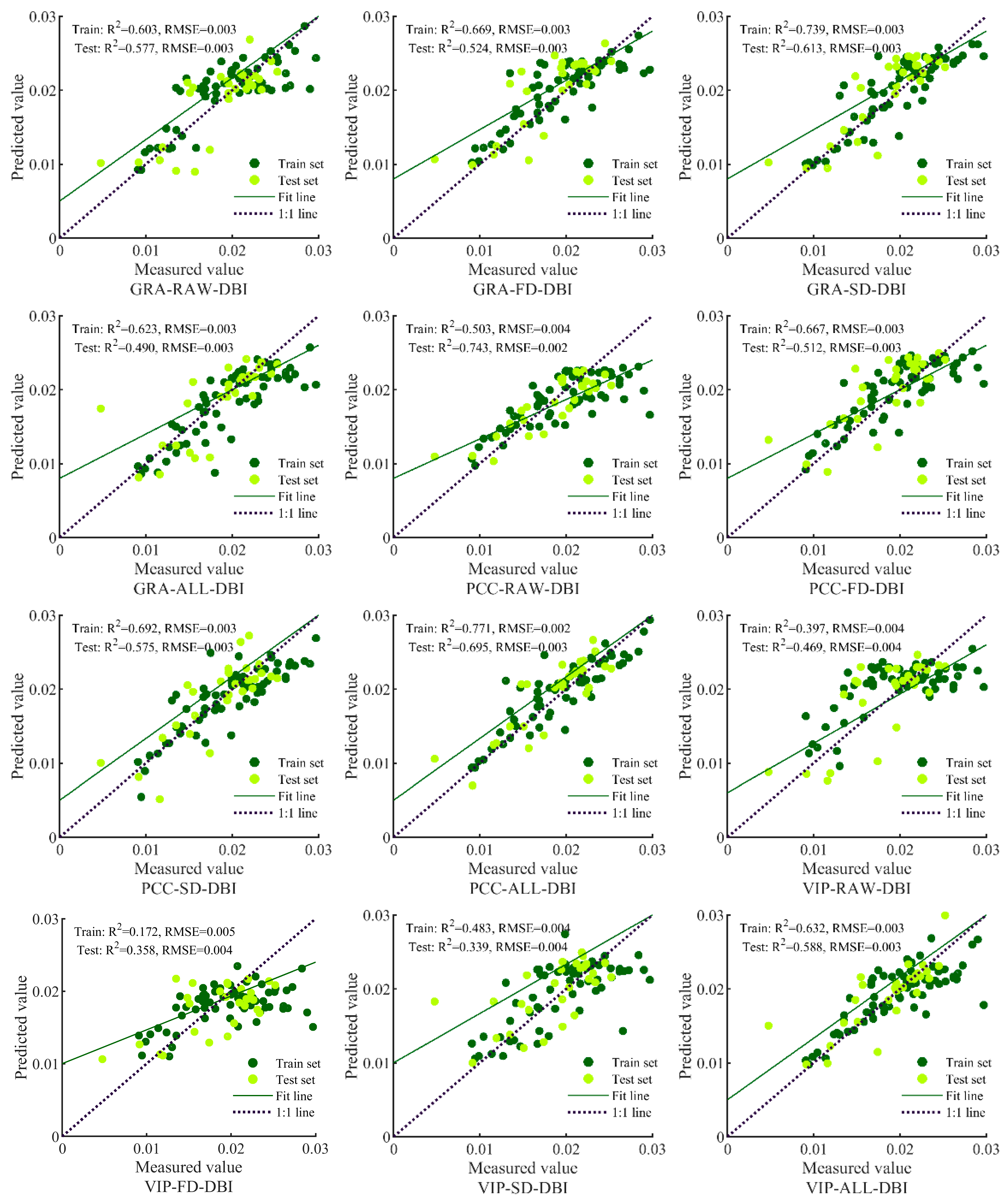
The scatter plots of observed versus predicted values for the Backpropagation neural network (BPNN) model are shown in Figure 8. The SD-GRA combination achieved the best validation accuracy (R2 = 0.613, RMSE = 0.0030), outperforming RAW-PCC (0.577), FD-VIP (0.524), and ALL (0.490). The ALL input caused overfitting and gave the poorest validation performance. Ranking: SD-GRA > RAW-PCC > FD-VIP > ALL.
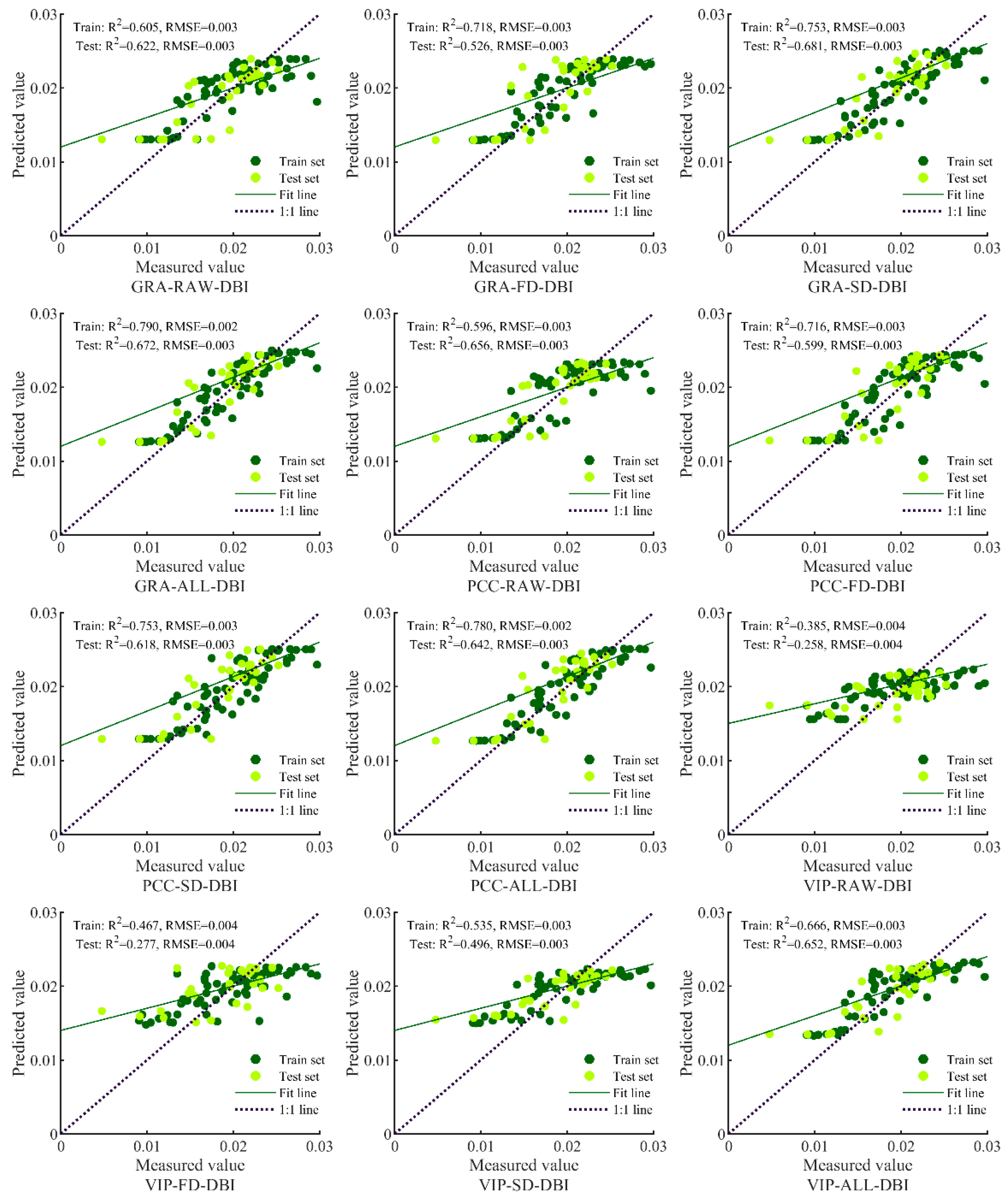
The scatter plots for the Random Forest (RF) model are shown in Figure 9. RAW-PCC and ALL-PCC performed best (R2 = 0.743 and 0.695, RMSE = 0.002–0.003), confirming RF’s robustness with high-dimensional data. FD-PCC and SD-PCC were weaker in validation. Ranking: RAW-PCC > ALL-PCC > FD-PCC > SD-PCC.
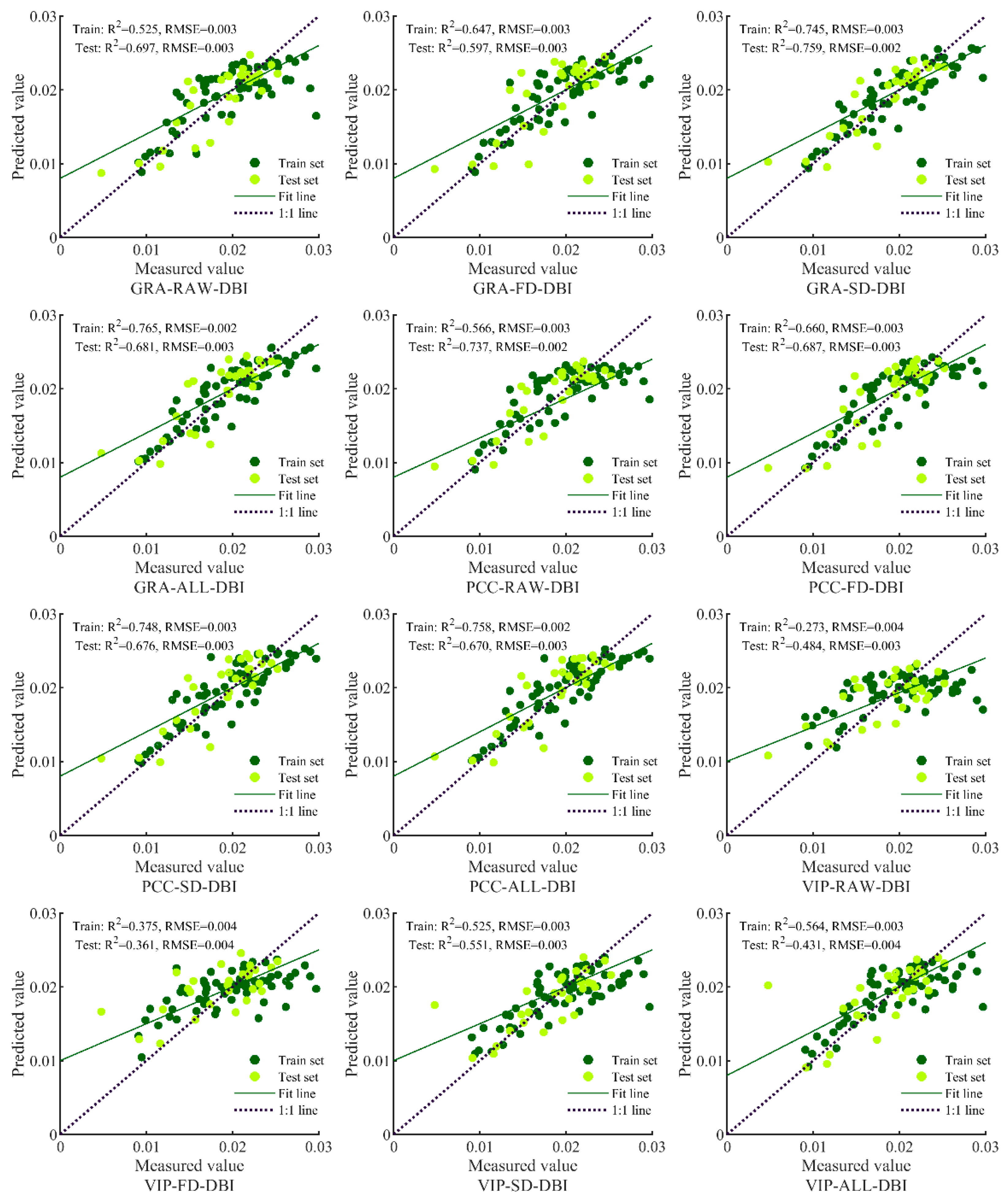
The scatter plots for the Support Vector Regression (SVR) model are shown in Figure 10. RAW and ALL combinations under PCC and VIP achieved high validation R2 (>0.72) with RMSE ≈ 0.002. The RAW-VIP combination was optimal (R2 = 0.729, RMSE = 0.002). Ranking: RAW-VIP > ALL-VIP > FD-VIP > SD-VIP.
Within each model family, SD-GRA performed best for BP, RAW-PCC for RF, and RAW-VIP for SVR. A comprehensive evaluation indicated that SD-VIP-SVR achieved the highest overall validation accuracy, whereas RAW-PCC-RF provided stable and robust performance across preprocessing scenarios (Table 3). Thus, SD-VIP-SVR can be regarded as the overall optimal pipeline, and RAW-PCC-RF as a robust and practical alternative for field applications.

4. Discussion

4.1. Impact of Spectral Index Types and Feature Selection Methods on Inversion Accuracy

Spectral index optimization proved decisive for maize nitrogen inversion, in line with evidence from wheat, rice, and soybean studies highlighting the red-edge region as critical for nitrogen retrieval [48,49,50]. In our work, NDI consistently outperformed SRI and DI across preprocessing scenarios, supporting Nikova et al.’s finding that normalized indices can reduce illumination and soil background interference via difference–sum operations [51]. Its improved performance after derivative preprocessing further suggests enhanced sensitivity to subtle chlorophyll and leaf structure variations, echoing results from cross-crop research [52,53,54]. Moreover, our results reinforce the physiological basis that nitrogen content strongly affects canopy chlorophyll concentration and leaf mesophyll scattering, which are most effectively captured by normalized indices in the 700–750 nm red-edge and 800–1000 nm NIR regions. Similar spectral–physiological linkages have been reported in rice and wheat, where derivative-enhanced NDIs captured subtle nitrogen-induced changes in pigment gradients and canopy internal multiple scattering.
In feature selection, PCC, GRA, and VIP displayed complementary advantages. PCC worked well with RF/SVR under RAW conditions, but has limitations with nonlinear relationships [55]. GRA captured trend similarity but was sensitive to noise under high dimensionality. VIP, built on the PLSR foundation, successfully identified cross-band contributions, and when paired with SVR, achieved the highest accuracy (R2 = 0.7593, RMSE = 0.0024), consistent with recent studies integrating hyperspectral and machine learning frameworks [56].

4.2. Applicability of Optimal Selection-Modeling Combinations

Our adaptability analysis showed PCC + RF (RAW) and VIP + SVR (SD) outperform most reported pipelines, even exceeding PCA + SVR benchmarks [57]. Mechanistically, RF’s ensemble learning mitigates PCC’s linear limitations, making it well-suited for field-scale monitoring, while VIP + SVR leverages nonlinear mapping to support precision fertilization applications, a pattern echoed in soybean and rice work using hyperspectral–ML approaches [58,59,60]. These findings also imply that integrating derivative preprocessing with nonlinear learning can better capture canopy spectral plasticity under variable illumination and background conditions. However, this study is constrained to maize in a single region and season. Broader multi-season, multi-crop validation is needed to assess robustness and transferability. Future work should combine deep learning and multi-source hyperspectral data (UAV, satellite) to enhance stability and expand applicability [61,62,63].

5. Conclusions

This study underscores the critical role of spectral index optimization in hyperspectral inversion of maize nitrogen content. Among the constructed indices—Normalized Difference Index (NDI), Simple Ratio Index (SRI), and Difference Index (DI)—NDI exhibited superior performance across preprocessing methods, consistent with earlier findings that normalized structures mitigate illumination and soil background effects [64,65]. Under original spectrum (RAW) conditions, the optimal NDI (700, 1801 nm) achieved a grey relational degree of 0.8947. After second-derivative (SD) preprocessing, the grey relational degree increased to 0.9077 (547, 551 nm), highlighting the advantage of normalized structures combined with derivative operations in enhancing nitrogen-sensitive features [66]. The three feature selection methods—Grey Relational Analysis (GRA), Pearson Correlation Coefficient (PCC), and Variable Importance in Projection (VIP)—demonstrated distinct adaptability but collectively improved modeling accuracy [67,68]. VIP excelled in Support Vector Regression (SVR) (SD preprocessing: test set R2 = 0.7593, RMSE = 0.0024); PCC showed the highest stability in Random Forest (RF) (RAW conditions: test set R2 = 0.6564, RMSE = 0.0028); and GRA was advantageous in BP neural networks with derivative features (SD preprocessing: test set R2 = 0.6134, RMSE = 0.0030). Overall, the SD-VIP-SVR combination achieved the highest inversion accuracy, representing the optimal model in this study. Spectral index optimization significantly enhances model reliability and generalization compared to full-spectrum input [69], serving as a key component and innovative contribution to hyperspectral technology applications in crop nitrogen monitoring. In addition, the optimized spectral–machine learning framework proposed in this study can be further applied to identify optimal nitrogen application rates, providing scientific guidance for precision fertilization and promoting sustainable nutrient management in agricultural production. Future studies should validate this pipeline across multiple seasons and crops to assess its broader applicability in precision fertilization systems [70].

Author Contributions

Investigation, data curation, methodology, visualization, software, writing—original draft preparation, Y.Z., H.L., and S.L.; validation, writing—review and editing, C.H. and J.L.; formal analysis, funding acquisition, C.H. and J.L.; resources, conceptualization, writing—review and editing, C.H. and J.L. All authors have read and agreed to the published version of the manuscript.

Funding

This study was supported by the Special project of scientific and technological innovation of Xinjiang Research Institute of Arid Area Agriculture: XJHQNY-2025-3, National Natural Science Foundation of China (No. 52309053), the Key Program of the Natural Science Foundation of Gansu Province (No. 24JRRA635), the Young Ph.D. Support Program of Colleges and Universities in Gansu Province (No. 2024QB-071), and the Discipline Team Project on Efficient Water Use and Water-Saving Mechanisms in Crops.

Institutional Review Board Statement

Not applicable.

Data Availability Statement

The original contributions presented in the study are included in the article. Further inquiries can be directed to the corresponding authors.

Acknowledgments

The authors wish to thank all those who helped in this research.

Conflicts of Interest

The authors declare no conflicts of interest.

References

  1. Chen, B.; Su, Q.; Li, Y.; Chen, R.; Yang, W.; Huang, C. Field rice growth monitoring and fertilization management based on uav spectral and deep image feature fusion. Agronomy 2025, 15, 886. [Google Scholar] [CrossRef]
  2. Wortman, S.E. Weedy fallow as an alternative strategy for reducing nitrogen loss from annual cropping systems. Agron. Sustain. Dev. 2016, 36, 61. [Google Scholar] [CrossRef]
  3. Ju, Z.; Liu, K.; Zhao, G.; Ma, X.; Jia, Z. Nitrogen fertilizer and sowing density affect flag leaf photosynthetic characteristics, grain yield, and yield components of oat in a semiarid region of northwest China. Agronomy 2022, 12, 2108. [Google Scholar] [CrossRef]
  4. Cox, W.E. Water Supply vs. the Environment: Finding the Appropriate Balance. In Critical Transitions in Water and Environmental Resources Management; Scientific Research Publishing Inc.: Salt Lake City, UT, USA, 2004; pp. 1–8. [Google Scholar]
  5. Chen, J.; Wang, G.; Hamani, A.K.M.; Amin, A.S.; Sun, W.; Zhang, Y.; Liu, Z.; Gao, Y. Optimization of Nitrogen fertilizer application with climate-smart agriculture in the North China Plain. Water 2021, 13, 3415. [Google Scholar] [CrossRef]
  6. Sandhu, N.; Sethi, M.; Kumar, A.; Dang, D.; Singh, J.; Chhuneja, P. Biochemical and genetic approaches improving nitrogen use efficiency in cereal crops: A review. Front. Plant Sci. 2021, 12, 657629. [Google Scholar] [CrossRef]
  7. Liu, J.; Feng, Z.; Mannan, A.; Khan, T.U.; Cheng, Z. Comparing non-destructive methods to estimate volume of three tree taxa in Beijing, China. Forests 2019, 10, 92. [Google Scholar] [CrossRef]
  8. Fu, S.; Meng, W.; Jeon, G.; Chehri, A.; Zhang, R.; Yang, X. Two-path network with feedback connections for pan-sharpening in remote sensing. Remote Sens. 2020, 12, 1674. [Google Scholar] [CrossRef]
  9. Yu, N.; Ren, B.; Zhao, B.; Liu, P.; Zhang, J. Leaf-nitrogen status affects grain yield formation through modification of spike differentiation in maize. Field Crops Res. 2021, 271, 108238. [Google Scholar] [CrossRef]
  10. Liu, L.; Huang, W.; Pu, R.; Wang, J. Detection of internal leaf structure deterioration using a new spectral Ratio index in the near-infrared shoulder region. J. Integr. Agr. 2014, 13, 760–769. [Google Scholar] [CrossRef]
  11. Jung, V.; Albert, C.H.; Violle, C.; Kunstler, G.; Loucougaray, G.; Spiegelberger, T. Intraspecific trait variability mediates the response of subalpine grassland communities to extreme drought events. J. Ecol. 2014, 102, 45–53. [Google Scholar] [CrossRef]
  12. Hu, Y.; Wang, X. Application of surrogate parameters in characteristic UV–vis absorption bands for rapid analysis of water contaminants. Sens. Actuators B Chem. 2017, 239, 718–726. [Google Scholar] [CrossRef]
  13. Somers, B.; Delalieux, S.; Verstraeten, W.W.; Eynde, A.V.; Barry, G.H.; Coppin, P. The contribution of the fruit component to the hyperspectral citrus canopy signal. Photogramm. Eng. Remote Sens. 2010, 76, 37–47. [Google Scholar] [CrossRef]
  14. Clevers, J.G.P.W.; Gitelson, A.A. Using the red-edge bands on Sentinel-2 for retrieving canopy chlorophyll and nitrogen content. In Proceedings of the First Sentinel-2 Preparatory Symposium, Frascati, Italy, 3–27 April 2012; Volume 707, p. 34. [Google Scholar]
  15. Clevers, J.G.; Gitelson, A.A. Remote estimation of crop and grass chlorophyll and nitrogen content using red-edge bands on Sentinel-2 and-3. Int. J. Appl. Earth. Obs. Geoinf. 2013, 23, 344–351. [Google Scholar] [CrossRef]
  16. Cao, C.L.; Wang, T.L.; Gao, M.F.; Li, Y.; Li, D.D.; Zhang, H.J. Hyperspectral Inversion of Nitrogen Content in Maize Leaves Based on Different Dimensionality Reduction Algorithms. Comput. Electron. Agric. 2021, 190, 106461. [Google Scholar] [CrossRef]
  17. Li, W.; Hou, Z.; Zhou, J.; Tao, R. SiamBAG: Band attention grouping-based Siamese object tracking network for hyperspectral videos. IEEE Trans. Geosci. Remote Sens. 2023, 61, 1–12. [Google Scholar] [CrossRef]
  18. Zhang, Z.; Jiang, D.; Chang, Q.; Zheng, Z.; Fu, X.; Li, K.; Mo, H. Estimation of anthocyanins in leaves of trees with apple mosaic disease based on hyperspectral data. Remote Sens. 2023, 15, 1732. [Google Scholar] [CrossRef]
  19. Anderson, L.O.; Aragao, L.E.; Shimabukuro, Y.E.; Almeida, S.; Huete, A. Fraction images for monitoring intra-annual phenology of different vegetation physiognomies in Amazonia. Int. J. Remote Sens. 2011, 32, 387–408. [Google Scholar] [CrossRef]
  20. Chen, C.; Liang, J.; Sun, W.; Yang, G.; Meng, X. An automatically recursive feature elimination method based on threshold decision in random forest classification. Geo-Spat. Inf. Sci. 2025, 28, 1494–1519. [Google Scholar] [CrossRef]
  21. Koh, J.C.; Banerjee, B.P.; Spangenberg, G.; Kant, S. Automated hyperspectral vegetation index derivation using a hyperparameter optimisation framework for high-throughput plant phenotyping. New Phytol. 2022, 233, 2659–2670. [Google Scholar] [CrossRef]
  22. Gitelson, A.A.; Merzlyak, M.N. Remote sensing of chlorophyll concentration in higher plant leaves. Adv. Space Res. 1998, 22, 689–692. [Google Scholar] [CrossRef]
  23. Xu, W.; Ma, R.; Zhou, Y.; Peng, S.; Hou, Y. Asymptotic properties of Pearson’s rank-variate correlation coefficient in bivariate normal model. Signal Process. 2016, 119, 190–202. [Google Scholar] [CrossRef]
  24. Han, J.; Guo, J.; Zhang, Z.; Yang, X.; Shi, Y.; Zhou, J. The rapid detection of trash content in seed cotton using near-infrared spectroscopy combined with characteristic wavelength selection. Agriculture 2023, 13, 1928. [Google Scholar] [CrossRef]
  25. Pei, J.; Xu, L.; Huang, Y.; Jiao, Q.; Yang, M.; Ma, D.; Jiang, S.; Li, H.; Li, Y.; Liu, S.; et al. A two-step simulated annealing algorithm for spectral data feature extraction. Sensors 2023, 23, 893. [Google Scholar] [CrossRef]
  26. Zhang, Y.; Xiao, J.; Yan, K.; Lu, X.; Li, W.; Tian, H.; Wang, L.; Deng, J.; Lan, Y. Advances and developments in monitoring and inversion of the biochemical information of crop nutrients based on hyperspectral technology. Agronomy 2023, 13, 2163. [Google Scholar] [CrossRef]
  27. Hou, Y.; Zhang, A.; Lv, R.; Zhao, S.; Ma, J.; Zhang, H.; Li, Z. A study on water quality parameters estimation for urban rivers based on ground hyperspectral remote sensing technology. Environ. Sci. Pollut. Res. 2022, 29, 63640–63654. [Google Scholar] [CrossRef]
  28. Morales, G.; Sheppard, J.W.; Logan, R.D.; Shaw, J.A. Hyperspectral dimensionality reduction based on inter-band redundancy analysis and greedy spectral selection. Remote Sens. 2021, 13, 3649. [Google Scholar] [CrossRef]
  29. Sales, M.H.R.; Souza, C.M.; Kyriakidis, P.C. Fusion of MODIS images using kriging with external drift. IEEE Trans. Geosci. Remote Sens. 2012, 51, 2250–2259. [Google Scholar] [CrossRef]
  30. Peng, X.; Li, J.; Wang, G.; Wu, Y.; Li, L.; Li, Z.; Bhatti, A.A.; Zhou, C.; Hepburn, D.M.; Reid, A.J.; et al. Random forest based optimal feature selection for partial discharge pattern recognition in HV cables. IEEE Trans. Power Deliv. 2019, 34, 1715–1724. [Google Scholar] [CrossRef]
  31. Zhang, J.; Dang, Q.; Malik, M. Baseline correction in parallel thorough QT studies. Drug Saf. 2013, 36, 441–453. [Google Scholar] [CrossRef]
  32. Chen, Y.; Song, Y.; Ma, J.; Zhao, J. Optimization-based scatter estimation using primary modulation for computed tomography. Med. Phys. 2016, 43 Pt 1, 4753–4767. [Google Scholar] [CrossRef]
  33. Ang, Y.S.; Ang, L.K. Current-temperature scaling for a Schottky interface with nonparabolic energy dispersion. Phys. Rev. Appl. 2016, 6, 034013. [Google Scholar] [CrossRef]
  34. Steinier, J.; Termonia, Y.; Deltour, J. Smoothing and differentiation of data by simplified least square procedure. Anal. Chem. 1972, 44, 1906–1909. [Google Scholar] [CrossRef]
  35. Cao, J.; Yang, H. A dynamic normalized difference index for estimating soil organic matter concentration using visible and near-infrared spectroscopy. Ecol. Indic. 2023, 147, 110037. [Google Scholar] [CrossRef]
  36. Massaoudi, M.; Refaat, S.S.; Abu-Rub, H.; Chihi, I.; Oueslati, F.S. PLS-CNN-BiLSTM: An End-to-End Algorithm-Based Savitzky–Golay Smoothing and Evolution Strategy for Load Forecasting. Energies 2020, 13, 20. [Google Scholar] [CrossRef]
  37. Rinnan, Å.; Van Den Berg, F.; Engelsen, S.B. Review of the most common pre-processing techniques for near-infrared spectra. Trac-Trend. Anal. Chem. 2009, 28, 1201–1222. [Google Scholar] [CrossRef]
  38. Robinson, N.P.; Allred, B.W.; Jones, M.O.; Moreno, A.; Kimball, J.S.; Naugle, D.E.; Erickson, T.A.; Richardson, A.D. A dynamic Landsat derived normalized difference vegetation index (NDVI) product for the conterminous United States. Remote Sens. 2017, 9, 863. [Google Scholar] [CrossRef]
  39. Fuyan, S.; Jing, L.; Wenjun, C.; Zhijun, T.; Weijing, M.; Suzhen, W.; Yongyong, X. Fatty liver disease index: A simple screening tool to facilitate diagnosis of nonalcoholic fatty liver disease in the Chinese population. Dig. Dis. Sci. 2013, 58, 3326–3334. [Google Scholar] [CrossRef] [PubMed]
  40. Chowdhury, A.R.; Kumbhakar, D.; Sarkar, S. Characterisation of a single mode trapezoidal index fiber by splice loss technique using lateral offset. Optik 2019, 178, 403–410. [Google Scholar] [CrossRef]
  41. Harrington, J.; Henninger-Voss, E.; Karhadkar, K.; Robinson, E.; Wong, T.W. Sum index and difference index of graphs. Discret. Appl. Math. 2023, 325, 262–283. [Google Scholar] [CrossRef]
  42. Yang, J.H.; Nie, J.J.; Fan, J.H. Relation of core dominance parameter and extended spectral index for radio sources. J. Astrophys. Astron. 2014, 35, 487–488. [Google Scholar] [CrossRef]
  43. Zhang, J.; Zhang, Q.; Zhang, J. The result greyness problem of the grey relational analysis and its solution. J. Intell. Fuzzy Syst. 2023, 44, 6079–6088. [Google Scholar] [CrossRef]
  44. Feng, W.; Zhu, Q.; Zhuang, J.; Yu, S. An expert recommendation algorithm based on Pearson correlation coefficient and FP-growth. Clust. Comput. 2019, 22 (Suppl. S3), 7401–7412. [Google Scholar] [CrossRef]
  45. Galindo-Prieto, B.; Trygg, J.; Geladi, P. A new approach for variable influence on projection (VIP) in O2PLS models. Chemometr. Intell. Lab. 2017, 160, 110–124. [Google Scholar] [CrossRef]
  46. Hu, Z.; Zhao, Q.; Wang, J. The prediction model of cotton yarn quality based on artificial recurrent neural network. In Proceedings of the International Conference on Applications and Techniques in Cyber Security and Intelligence, Huainan, China, 22–24 June 2019; Springer International Publishing: Cham, Switzerland, 2019; pp. 857–866. [Google Scholar]
  47. Wahjudi, A.; Salamoni, T.D.; Batan, I.M.L.; Harnany, D. Determination of injection molding process parameters using combination of backpropagation neural network and genetic algorithm optimization method. Int. J. Mech. Eng. Sci. 2021, 5, 39–44. [Google Scholar] [CrossRef]
  48. Zhang, W.; Zhang, L.; Yang, J.; Hao, X.; Guan, G.; Gao, Z. An experimental modeling of cyclone separator efficiency with PCA-PSO-SVR algorithm. Powder Technol. 2019, 347, 114–124. [Google Scholar] [CrossRef]
  49. Marshall, M.; Belgiu, M.; Boschetti, M.; Pepe, M.; Stein, A.; Nelson, A. Field-level crop yield estimation with PRISMA and Sentinel-2. Isprs. J. Photogramm. 2022, 187, 191–210. [Google Scholar] [CrossRef]
  50. Gao, J.S.; Li, J.M.; Xu, M.G.; Sun, N.; Qin, D.Z. The Effects of longEterm chemical fertilizers on yield of upland crops and paddy rice in red soil. Chin. Agric. Sci. Bull. 2008, 24, 286–292. [Google Scholar]
  51. Ng, A.; Soo, K. Random forests. In Data Science–Was Ist Das Eigentlich?! Algorithmen Des Maschinellen Lernens Verständlich Erklärt; Springer: Berlin/Heidelberg, Germany, 2018; pp. 117–127. [Google Scholar]
  52. Nikova, I.; Atanassova, S.; Tanev, S. Normalized indices for minimizing illumination and soil background effects in crop spectral monitoring. Comput. Electron. Agric. 2014, 103, 1–10. [Google Scholar]
  53. Li, F.; Mistele, B.; Hu, Y.; Chen, X.; Schmidhalter, U. Reflectance estimation of canopy nitrogen content in winter wheat using optimised hyperspectral spectral indices and partial least squares regression. Eur. J. Agron. 2014, 52, 198–209. [Google Scholar] [CrossRef]
  54. Sun, J.; Yang, J.; Shi, S.; Chen, B.; Du, L.; Gong, W.; Song, S. Estimating rice leaf nitrogen concentration: Influence of regression algorithms based on passive and active leaf reflectance. Remote Sens. 2017, 9, 951. [Google Scholar] [CrossRef]
  55. Pandey, P.; Ge, Y.; Stoerger, V.; Schnable, J.C. High throughput in vivo analysis of plant leaf chemical properties using hyperspectral imaging. Front. Plant Sci. 2017, 8, 1348. [Google Scholar] [CrossRef]
  56. Pullanagari, R.R.; Yule, I.J.; Hedley, M.J.; Tuohy, M.P.; Dynes, R.A.; King, W.M. Multi-spectral radiometry to estimate pasture quality components. Precis. Agric. 2012, 13, 442–456. [Google Scholar] [CrossRef]
  57. Carlier, A.; Dandrifosse, S.; Dumont, B.; Mercatoris, B. Comparing CNNs and PLSr for estimating wheat organs biophysical variables using proximal sensing. Front. Plant Sci. 2023, 14, 1204791. [Google Scholar] [CrossRef] [PubMed]
  58. Hogan, J.B. Plant-based diets in kidney disease management. Dial. Transplant. 2011, 40, 407–409. [Google Scholar] [CrossRef]
  59. Tao, L.I.U.; Fengyuan, Y.A.N.G.; Wang, L.I.U.; Dongmei, Y.I.N.; Youzhou, J.I.A.O. Estimation of peanut biomass based on feature selection and particle swarm optimization. Trans. Chin. Soc. Agric. Eng. 2025, 41, 238–247. [Google Scholar]
  60. Radoglou-Grammatikis, P.; Sarigiannidis, P.; Lagkas, T.; Moscholios, I. A compilation of UAV applications for precision agriculture. Comput. Netw. 2020, 172, 107148. [Google Scholar] [CrossRef]
  61. Sishodia, R.P.; Ray, R.L.; Singh, S.K. Applications of remote sensing in precision agriculture: A review. Remote Sens. 2020, 12, 3136. [Google Scholar] [CrossRef]
  62. Wan, Y.; Zhong, Y.; Ma, A.; Hu, X.; Wei, L. Satellite-air-ground integrated multi-source earth observation and machine learning processing brain for tailings reservoir monitoring and rapid emergency response. Land Degrad. Dev. 2023, 34, 1941–1959. [Google Scholar] [CrossRef]
  63. Vu, A.D.; Nguyen, K.V.; Bui, B.Q.; Kamel, N. A comprehensive survey of super-resolution remote sensing image datasets: Evolution, challenges, and future directions. IEEE Access 2025, 13, 145350–145372. [Google Scholar] [CrossRef]
  64. Jiang, Y.; Zhang, L.; Yan, M.; Qi, J.; Fu, T.; Fan, S.; Chen, B. High-resolution mangrove forests classification with machine learning using worldview and UAV hyperspectral data. Remote Sens. 2021, 13, 1529. [Google Scholar] [CrossRef]
  65. Gitelson, A.A.; Viña, A.; Ciganda, V.; Rundquist, D.C.; Arkebauer, T.J. Remote estimation of canopy chlorophyll content in crops. Geophys. Res. Lett. 2005, 32, L08403. [Google Scholar] [CrossRef]
  66. Boerjan, W. Lignin Management: Optimizing Yield and Composition in Lignin-Modified Plants. GCEP (Y1, partial) Report. 2014, pp. 1–20. Available online: https://d1wqtxts1xzle7.cloudfront.net/76564755/2.3.4_Chapple_Sponsor_and_Public_Version-libre.pdf (accessed on 13 August 2025).
  67. Fu, Y.; Yang, G.; Pu, R.; Li, Z.; Li, H.; Xu, X.; Song, X.; Yang, X.; Zhao, C. An overview of crop nitrogen status assessment using hyperspectral remote sensing: Current status and perspectives. Eur. J. Agron. 2021, 124, 126241. [Google Scholar] [CrossRef]
  68. Chen, Y.; Shahidehpour, M.; Lin, Y.; Dvorkin, Y.; Peric, V.; Zhao, J.; Ugalde-Loo, C.E.; Ge, L. Guest Editorial: Situational awareness of integrated energy systems. IET Gener. Transm. Dis. 2022, 16, 2761–2765. [Google Scholar] [CrossRef]
  69. Zhang, Z.; Wang, Z.; Luo, Y.; Zhang, J.; Chen, Y.; Peng, C.; Ye, K.; Lin, W.; Zhang, J.; Wang, Y.; et al. Quantifying heavy metal concentrations in industrial-transitional zone soils via integrated XRF and VIS-NIR spectroscopy. Environ. Pollut. 2025, 384, 127015. [Google Scholar] [CrossRef] [PubMed]
  70. Liu, X.; Feng, X.; Liu, F.; He, Y. Identification of hybrid rice strain based on near-infrared hyperspectral imaging technology. Trans. Chin. Soc. Agric. Eng. 2017, 33, 189–194. [Google Scholar]
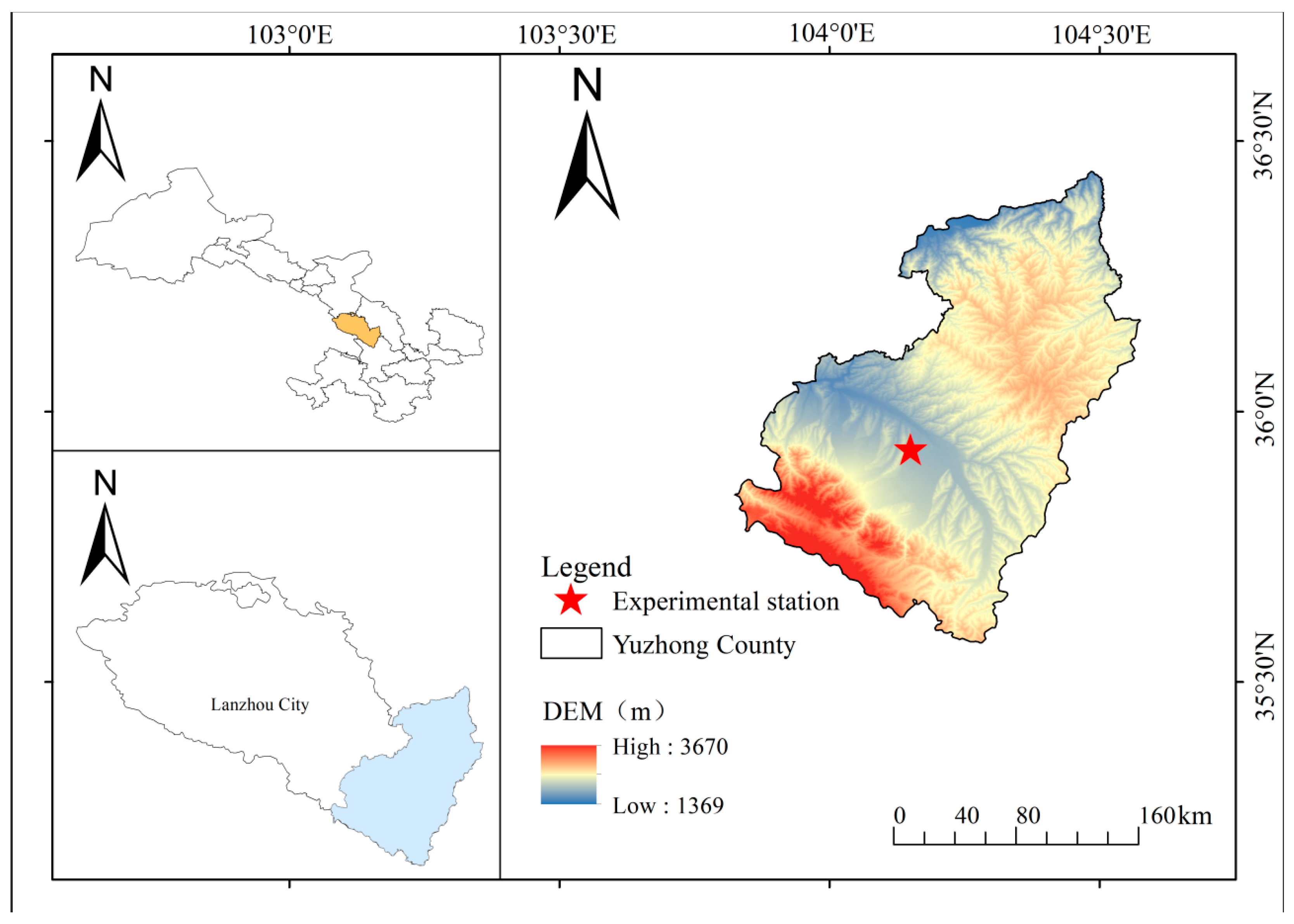
Figure 1. Overview map of the study area. All figures and tables were generated by the authors based on the experimental data of this study.
Agronomy 15 02485 g001
Figure 2. The methodological workflow diagram for this study.
Agronomy 15 02485 g002
Figure 3. Maximum correlation coefficients between different preprocessing methods and maize nitrogen content.
Agronomy 15 02485 g003
Figure 4. Spectral curves of the maize canopy. (a) Original spectrum. (b) First derivative (FD). (c) Second derivative (SD).
Agronomy 15 02485 g004
Figure 5. Two-dimensional determination coefficient matrix diagram: (a) RAW-DI-GRA; (b) RAW-SRI-GRA; (c) RAW-NDI-GRA; (d) FD-DI-GRA; (e) FD-SRI-GRA; (f) FD-NDI-GRA; (g) SD-DI-GRA; (h) SD-SRI-GRA; (i) SD-NDI-GRA.
Agronomy 15 02485 g005
Figure 6. Two-dimensional determination coefficient matrix diagram: (a) RAW-DI-PCC; (b) RAW-SRI-PCC; (c) RAW-NDI-PCC; (d) FD-DI-PCC; (e) FD-SRI-PCC; (f) FD-NDI-PCC; (g) SD-DI-PCC; (h) SD-SRI-PCC; (i) SD-NDI-PCC.
Agronomy 15 02485 g006
Figure 7. Two-dimensional determination coefficient matrix diagram: (a) RAW-DI-VIP; (b) RAW-SRI- VIP; (c) RAW-NDI-VIP; (d) FD-DI-VIP; (e) FD-SRI-VIP; (f) FD-NDI-VIP; (g) SD-DI-VIP; (h) SD-SRI-VIP; (i) SD-NDI-VIP.
Agronomy 15 02485 g007
Figure 8. Scatter plot of observed versus predicted values for the BPNN model.
Agronomy 15 02485 g008
Figure 9. Scatter plot of observed versus predicted values for the RF model.
Agronomy 15 02485 g009
Figure 10. Scatter plot of observed versus predicted values for the SVR model.
Agronomy 15 02485 g010
Table 1. Preprocessing methods of spectral data.
Preprocessing Method [35]CategoryAbbreviationMain Function
RAWRaw reflectanceRAWOriginal spectral data without any processing
StandardizationMin–Max scalingMMSScales values into the range [0, 1]
Z-score scalingZ-ScoreStandardizes data to zero mean and unit variance
NormalizationNormalizeNormalizes samples to eliminate scale differences
SmoothingMoving averageMovingAvgReduces noise and smooths spectral curves
Savitzky–Golay smoothing [36]SGSmooths spectra while preserving curve shape
Scatter correctionMultiplicative scatter correctionMSCCorrects scattering and particle size effects
Standard normal variateSNVReduces variability caused by scatter differences
Derivative transformFirst derivativeFDEnhances slope changes and highlights spectral inflection points
Second derivativeSDStrengthens spectral features and improves resolution
Baseline correctionDetrendDetrendRemoves baseline drift and background trends
Table 2. Optimal wavelength positions and performance metrics (GRA degree, Pearson correlation coefficient, and VIP score) of spectral indices with respect to nitrogen content.
Feature Selection StrategiesProcessing MethodDI Optimal Wavelength Position (i, j)/nmMax(ξ/r/Score)SRI Optimal Wavelength Position (i, j)/nmMax(ξ/r/Score)NDI Optimal Wavelength Position (i, j)/nmMax(ξ/r/Score)
GRARAW(718, 1726)0.8717(702, 1801)0.8851(700, 1801)0.8947
FD(685, 1507)0.8809(746, 1126)0.8876(679, 1639)0.9037
SD(646, 612)0.8923(750, 1155)0.8939(547, 551)0.9077
PCCRAW(493, 492)0.7510(1743, 707)0.7797(1743, 707)0.7771
FD(1566, 684)0.7949(1333, 734)0.8228(1566, 683)0.7991
SD(646, 612)0.8112(547,551)0.8313(551, 547)0.8295
VIPRAW(1344, 725)1(1595, 1596)1(1595, 1596)1
FD(714, 705)1(1094, 671)1(1296, 1071)1
SD(1153, 721)1(1778, 2398)1(2121, 473)1
Table 3. Summarizes the variables used in each modeling method and the corresponding R2 values with 95% confidence intervals.
Input VariableModel MethodTrainTest
R295% CIRMSER295% CIRMSE
GRA-RAW-DBIBPNN0.6034[0.4292, 0.7382]0.00310.5774[0.2852, 0.7823]0.0032
RF0.6046[0.4306, 0.7391]0.00320.6223[0.3409, 0.8087]0.0030
SVR0.5250[0.3377, 0.6795]0.00350.6972[0.4441, 0.8507]0.0027
GRA-FD-DBIBPNN0.6693[0.5117, 0.7854]0.00290.5237[0.2247, 0.7493]0.0034
RF0.7178[0.5757, 0.8191]0.00270.5257[0.2268, 0.7506]0.0033
SVR0.6470[0.4832, 0.7696]0.00300.5966[0.3085, 0.7937]0.0031
GRA-SD-DBIBPNN0.7387[0.6041, 0.8333]0.00260.6134[0.3295, 0.8036]0.0030
RF0.7526[0.6232, 0.8427]0.00250.6808[0.4204, 0.8417]0.0027
SVR0.7454[0.6133, 0.8378]0.00250.7593[0.5397, 0.8838]0.0024
GRA-ALL-DBIBPNN0.6227[0.4427, 0.7580]0.00310.4901[0.1479, 0.7553]0.0035
RF0.7900[0.6685, 0.8710]0.00230.6716[0.3602, 0.8542]0.0028
SVR0.7652[0.6328, 0.8549]0.00240.6813[0.3741, 0.8590]0.0027
PCC-RAW-DBIBPNN0.5031[0.3135, 0.6626]0.00360.7432[0.5140, 0.8753]0.0025
RF0.5959[0.4201, 0.7327]0.00320.6564[0.3863, 0.8281]0.0028
SVR0.5661[0.3847, 0.7107]0.00330.7366[0.5037, 0.8719]0.0025
PCC-FD-DBIBPNN0.6668[0.5085, 0.7837]0.00290.5116[0.2120, 0.7417]0.0034
RF0.7156[0.5727, 0.8176]0.00270.5991[0.3116, 0.7952]0.0031
SVR0.6598[0.4995, 0.7787]0.00290.6866[0.4287, 0.8449]0.0027
PCC-SD-DBIBPNN0.6925[0.5420, 0.8016]0.00280.5755[0.2830, 0.7812]0.0032
RF0.7526[0.6232, 0.8427]0.00250.6181[0.3355, 0.8063]0.0030
SVR0.7480[0.6169, 0.8396]0.00250.6765[0.4143, 0.8393]0.0028
PCC-ALL-DBIBPNN0.7713[0.6415, 0.8588]0.77130.6950[0.3944, 0.8658]0.0027
RF0.7798[0.6537, 0.8644]0.00240.6422[0.3195, 0.8393]0.0029
SVR0.7579[0.6225, 0.8501]0.00250.6703[0.3583, 0.8536]0.0028
VIP-RAW-DBIBPNN0.3971[0.2053, 0.5766]0.00390.4694[0.1702, 0.7142]0.0035
RF0.3846[0.1936, 0.5660]0.00400.2584[0.0253, 0.5543]0.0042
SVR0.2727[0.0994, 0.4648]0.00430.4844[0.1846, 0.7241]0.0035
VIP-FD-DBIBPNN0.1715[0.0344, 0.3604]0.00460.3575[0.0795, 0.6350]0.0039
RF0.4672[0.2752, 0.6343]0.00370.2771[0.0335, 0.5705]0.0041
SVR0.3748[0.1846, 0.5576]0.00400.3613[0.0821, 0.6379]0.0039
VIP-SD-DBIBPNN0.4826[0.2914, 0.6465]0.00360.3387[0.0672, 0.6206]0.0039
RF0.5353[0.3493, 0.6874]0.00340.4957[0.1957, 0.7315]0.0034
SVR0.5250[0.3377, 0.6795]0.00350.5512[0.2549, 0.7664]0.0033
VIP-ALL-DBIBPNN0.6321[0.4545, 0.7647]0.00270.5882[0.2512, 0.8109]0.0031
RF0.6665[0.4985, 0.7886]0.00290.6519[0.3326, 0.8443]0.0029
SVR0.5643[0.3721, 0.7160]0.00330.4306[0.0981, 0.7187]0.0037
Disclaimer/Publisher’s Note: The statements, opinions and data contained in all publications are solely those of the individual author(s) and contributor(s) and not of MDPI and/or the editor(s). MDPI and/or the editor(s) disclaim responsibility for any injury to people or property resulting from any ideas, methods, instructions or products referred to in the content.