Article

Non-Destructive Estimation of Area and Greenness in Leaf and Seedling Scales: A Case Study in Cucumber

by
Georgios Tsaniklidis
1,†,
Theodora Makraki
1,†,
Dimitrios Papadimitriou
2,
Nikolaos Nikoloudakis
3,*,
Amin Taheri-Garavand
4 and
Dimitrios Fanourakis
5,*
1
Institute of Olive Tree, Subtropical Plants and Viticulture, Hellenic Agricultural Organization ‘ELGO-Dimitra’, Kastorias 32A, 71307 Heraklion, Greece
2
Laboratory of Natural Resources Management & Agricultural Engineering, Department of Agriculture, Hellenic Mediterranean University, Estavromenos, 71410 Heraklion, Greece
3
Department of Agricultural Science, Biotechnology and Food Science, Cyprus University of Technology, Limassol 3036, Cyprus
4
Mechanical Engineering of Biosystems Department, Lorestan University, Khorramabad P.O. Box 465, Iran
5
Laboratory of Quality and Safety of Agricultural Products, Landscape and Environment, Department of Agriculture, School of Agricultural Sciences, Hellenic Mediterranean University, Estavromenos, 71004 Heraklion, Greece
*
Authors to whom correspondence should be addressed.
These authors contributed equally to this work.
Agronomy 2025, 15(10), 2294; https://doi.org/10.3390/agronomy15102294
Submission received: 30 August 2025 / Revised: 21 September 2025 / Accepted: 24 September 2025 / Published: 28 September 2025
(This article belongs to the Special Issue Smart Agriculture for Crop Phenotyping)

Abstract

Leaf area (LA) and SPAD value (a proxy for chlorophyll content) are two key determinants of seedling quality. This study aimed to develop and validate approaches for the efficient retrieval of these features in order to facilitate both management and screening practices. In cucumber, different models were developed and tested for the accurate estimation of LA at the scale of the individual organ (cotyledon, leaf) by using its linear dimensions (length (L) and width (W)), and of the whole seedling by using the 2D image-extracted projected area (from three different angles: 0°, 45°, and 90°). At either scale, the SPAD value was computed by using image (90°)-based colorimetric features. The estimation of individual organ area was more accurate when using L alone, compared with W alone. By using the two dimensions and specific colorimetric features, the individual organ area (R2 ≥ 0.92) and SPAD value (R2 of 0.77) were accurately predicted. When considering a single view, the top one (90°) was associated with the highest accuracy in whole-seedling LA estimation, and the side view (0°) with the lowest (R2 of 0.88 and 0.73, respectively). Using any combination of two angles, the whole-seedling LA was accurately retrieved (R2 ≥ 0.88). When using colorimetric features, a poor estimation of the whole-seedling SPAD value was noted (R2 ≤ 0.43). The deployment of artificial neural networks (ANNs) further allowed the estimation of specific organ shape traits, and improved the accuracy of all the aforementioned predictions, including the whole-seedling SPAD value (R2 of 0.597). In conclusion, the findings of this study highlight that features readily retrieved from 2D images hold promising potential for improving screening routines within the nursery industry.

1. Introduction

On a global scale, both crop productivity and end-product quality strongly rely on the early phase of plant development [1]. Compared with directly seeded plants, high-quality young plants (the so-called seedlings, commercially designated as transplants) are associated with an array of benefits, including improved earliness and total yield, as well as enhanced tolerance to stress [2]. In this context, this initial phase directly impacts the efficiency of the subsequent (agricultural and horticultural) practices, the fitness of adult plants, and, eventually, the overall crop success. Therefore, developing non-destructive techniques for the selection and mass screening of essential seedling traits is clearly in demand.
Leaves are primarily involved in light interception, water/carbon balance, and thermal exchange [3,4]. In this perspective, the seedling leaf area (LA) represents one of the most important elements of their quality, as it is directly linked to plant establishment, growth, and yield [5,6]. The whole-seedling LA is estimated by adding together the areas of two cotyledons and all true leaves (typically up to four, always including expanding ones). The toolbox available for evaluating the area of individual organs (cotyledons, leaves) is rather limited. The most accessible option is possibly the use of a scanning planimeter (such as Li-3100, LI-COR, Lincoln, NE, USA). This method is mostly precise but not in all cases (e.g., not for small and (or) narrow leaves, or for not entirely flat laminae) [7]. Additionally, it is invasive (i.e., herbal material needs to be excised from the seedling) and time-consuming (thus limited in scale), while the equipment involved is non-portable and prohibitively expensive. At the individual-organ scale, an alternative non-invasive option is to develop a mathematical prediction model that estimates LA as a function of leaf dimensions (length (L) and (or) width (W)) for the species of interest [8,9,10]. These models typically focus on fully expanded leaves [11,12], possibly limiting their applicability to the study of adult plants, as in the seedling case scenario (including developing leaves), errors may arise. Consequently, additional assessments should be performed on a case-by-case basis encompassing different leaf developmental stages. Additionally, to the best of our knowledge, there are no models focusing on cotyledons, which are a significant contributor to whole-seedling area, especially in the early stage [13]. At the whole-plant scale, digital-image-based areas have been found to be adequately related to plant LA in a few species, with the accuracy of this estimation being dependent on the number of images and the angle between them [4,14].
Seedling greenness is another key indicator of quality and is a function of leaf chlorophyll content [5,15]. Leaf chlorophyll content is directly associated with nitrogen status and photosynthetic capacity, while it is highly sensitive to both biotic and abiotic stresses [4,16]. Chlorophyll content assessments are typically conducted though spectrophotometry, which is a destructive and inefficient protocol. To overcome this bottleneck, chlorophyll content determinations are conventionally performed via chlorophyll meters (such as SPAD-502; Minolta, Tokyo, Japan) [17,18]. Notwithstanding their utility, a representative SPAD value of a single leaf is the average of multiple readings (the number depending on its size and uniformity) [16]. At the whole-plant scale, several leaves ought to be considered, owing to vertical variation such as the difference between developing leaves (top layer) and fully developed ones, evidently representing a more biologically and technically relevant measure of plant health and (or) stress level [19]. At the individual-organ scale, color features extracted from images have previously been shown to be related to chlorophyll content in soybean [20] and rice [21]. However, given interspecific differences in leaf characteristics (e.g., cuticle and trichome morphology), which regulate the reflectance patterns, the respective relationship is species-specific [22]. Instead, work devoted to the whole plant is limited owing to difficulties arising from the three-dimensional (3D) structure.
Recent years have witnessed the growing deployment of artificial neural networks (ANNs) in phenotyping plant traits [23,24,25]. Owing to their capacity to discriminate patterns and derive regularities from data, ANNs have led to significant progress in the exploration of complicated concepts [26,27]. By testing an array of linear, non-linear, and ANN models, the present study aimed (i) to predict the area of individual organs (cotyledons and true leaves) from their linear dimensions (L and/or W) and, by applying ANNs, the potential to retrieve additional morphometric traits (e.g., perimeter, petiole length); (ii) to estimate the whole-seedling leaf area from the image-based projected area acquired from three different viewing angles (0°, 45°, and 90°), thereby evaluating the effect of viewing geometry on estimation accuracy and testing combinations of angles to mitigate occlusion/self-shading; and (iii) to predict both the individual-organ and whole-seedling SPAD values (a proxy for chlorophyll content) by employing image-based colorimetric features extracted from digital images, and to identify which color metrics provide the strongest predictive power. Cucumber (Cucumis sativus L.) was chosen as a model species owing to its large social and economic impact around the globe. Variation in organ and seedling features was introduced by differences in environmental and cultivation conditions, as well as by sampling different developmental stages (growth duration).

2. Materials and Methods

2.1. Plant Material and Growth Conditions

Seeds of cucumber (Cucumis sativus L.) ‘Aisopos’ F1 RZ were acquired from a commercial source (Rijk Zwaan, De Lier, The Netherlands). Prior to further use, seed surface sterilization was practiced by immersion in sodium hypochlorite solution (2%, v/v) for 2 min. To detach any surface-adhered traces of the sterilization agent, seeds were thoroughly washed with sterile deionized water. Seeds were gently arranged between two layers of moist filter paper on a tray, taking care to avoid excess pressure. Subsequently, the tray was covered with a layer of wax paper to prevent moisture loss. Germination was undertaken in an incubator under constant temperature (30 °C) and darkness. Radicle emergence was classified as positive germination. Seeds of radicle length within a given range (4–8 mm) were used for experimentation. Following sieving (4 mm), 0.22 L black square pots (l × w × h = 7 × 7 × 6 cm) were filled by weight (115 g pot−1) with a commercial nutrient-enriched substrate (Compo Sana, Compo, Münster, Germany). At potting, growth media water content (3 g g−1) was homogeneous within and between pots. Pregerminated seeds were manually planted at a constant sowing depth (4 mm). One seed was deposited per pot. Planted pots were placed on trays (l × w × h = 85 × 35 × 8 cm), at a density of 110 pots m−2. This density is within the range which is employed in commercial seedling production facilities [1,2]. The trays were randomly allocated in a greenhouse compartment (Heraklion; 35.3° N, 25.1° E) on three tables. Pots were regularly irrigated from below to the pot capacity (EC of 0.76 dS m−1). The period between the sowing and cotyledon stage (i.e., fully open cotyledons prior to the emergence of the first leaf) was 10 d. Seedlings were cultivated for additional 5 weeks.
At 21 d, three treatments were additionally imposed, including suboptimal temperature (10 °C and darkness for 24 h), salinity (irrigation with an EC of 5 dS m−1), and flooding (pots submerged in water for 5 d). Cultivation was conducted under naturally fluctuating conditions of air temperature (18.6 ± 0.3 °C), relative air humidity (62.6 ± 1.1%) and daily light integral (10.1 ± 0.4 mol m−2 d−1).
Assessments were initiated at the cotyledon stage (time 0), and continued for 35 d (7, 14, 21, and 35 d). At 35 d, seedlings had developed up to 4 leaves. The employed range of growth period (and thus of number of leaves (seedling−1)) covers the variation in the cultivation span which is typically encountered under commercial production and distribution settings [1,2]. At each time point, seedlings were randomly selected for measurements. Cotyledon, leaf, and whole-seedling scales were considered. At each seedling, cotyledons and all unfolded leaves (encompassing different developmental stages) were evaluated. Before undertaking the destructive sampling, cotyledon and leaf SPAD values were obtained within 2 h after the onset of the light period οn intact seedlings, followed by whole-seedling images (under 3 different viewing angles). Hence, the same group of seedlings was employed for assessments at both organ (cotyledon, leaf) and whole-seedling levels (n = 630).
The robustness to both genetic (intraspecies) and environmentally induced variability of the conventional mathematical models for area estimation at both organ (cotyledon, leaf) and whole-seedling levels under development was challenged. In this perspective, these mathematical models were validated by employing another 8 cucumber cultivars (obtained from different commercial sources) and 2 cucumber traditional varieties (from an ongoing research project; Supplementary Table S1) as test material. Based on preliminary observations, these 10 cucumber genotypes were chosen to cover the largest possible variation in both leaf shape and seedling architecture. At assessment, seedlings had developed between 2 to 4 leaves. The same sets of seedlings were used for evaluations at both organ (cotyledon, leaf) and whole-seedling levels (n = 10).

2.2. Morphometric and Colorimetric Analysis of Individual Cotyledons and Leaves

Cotyledons and leaves were carefully excised from the seedlings. To achieve accurate area and shape information, potential folds were avoided. On this basis, samples were flattened by placing them between two acrylic sheets (l × w × thickness = 297 × 210 × 3 mm; 50 g) for 20 min. The upper sheet was transparent. The lower sheet was white (employed as the background during imaging). Herbal material was photographed using a custom-built imaging station (l × w × h = 44 × 44 × 44 cm; prototype I). To maintain consistent and defined illumination conditions, an artificial lighting system (4000 K white light-emitting diode, 0.4 m; Philips, Eindhoven, The Netherlands) was installed at the inside top of the station. To enhance light reflectivity and ensure an even light distribution, the interior of the imaging station was painted white. Images were captured through a circular aperture (diameter of 8 cm), which was positioned at the center of the upper side. The camera-to-sample distance was kept constant at 36 cm. Samples were manually inserted by opening a door providing access to the image acquisition station. To avoid light pollution, the imaging station door was always closed during image acquisition, and operation was conducted in a dark room. Samples were imaged under a white background. With the adaxial (upper) side facing up, every sample was captured once in the vertical downward direction towards it (i.e., image plane parallel to the lamina surface). Each image included a scale indicator (a ruler). Two-dimensional (2D) images were recorded using a charge-coupled device (CCD) digital camera (PowerShot G15, 12 megapixels; Canon, Tokyo, Japan). Across evaluation, image capture settings [resolution of 12 megapixels, f-stop of 2.8, shutter speed (exposure time) of 1/100 s, ISO speed of 800 (ISO-800), without flash/zoom] were identical. The images were acquired in the RGB color space and saved in JPEG format (resolution of 4000 × 3000 pixels).
In cotyledons, L (from base to top along middle vein; major axis), W (widest point along the transverse axis perpendicular to the longitudinal one; minor axis), perimeter (length of the path enclosing the outline along the margins (edges)), and area (one-sided planar surface area) were digitally recorded (ImageJ, version 1.53e; Wayne Rasband/NIH, Bethesda, MD, USA; Figure 1 and Table 1). In leaves, petiole (stalk) L (Lp; from petiole base to leaf base), petiole area, lamina (blade) L (from base to top along middle vein), leaf L (i.e., Lp + lamina length), W, perimeter, and LA (i.e., petiole area + lamina area) were determined (Figure 1 and Table 1). Dimension and area values were recorded to the resolution of 1 mm and 1 mm2, respectively.
In cotyledons and leaves, outlines were digitally analyzed (ImageJ, version 1.53e; Wayne Rasband/NIH, Bethesda, MD, USA) to compute the following four (dimensionless) quantitative indices of leaf shape: (I) aspect ratio (ratio of major to minor axes of the best-fitted ellipse), (II) circularity [ 4 π × a r e a ( p e r i m e t e r ) 2 ], (III) roundness [ 4 × a r e a 4 π × ( m a j o r a x i s ) 2 ], and (IV) solidity [ a r e a c o n v e x   a r e a ] ([7], see Table 1). Each index represents a discrete feature of shape. The first two (aspect ratio, roundness) are sensitive to the ratio of L to W, while the latter two (circularity, solidity) are affected by serration (saw-like edges) and lobing (dissection) [28]. Aspect ratio extends from 1 to a theoretical infinity (corresponding to circle and infinitely narrow, respectively). Roundness and circularity increase from 0 to 1 (corresponding to an infinitely narrow shape and a circle, respectively). Solidity increases from 0 to 1, exhibiting an inversely proportional response to boundary irregularities. For leaves, two additional shape features (ratios of petiole to leaf length and of petiole to leaf area) were calculated (see Table 1).
In cotyledons and leaves, the captured displays were digitally processed (Trigit [29]) for the acquisition of colorimetric features in the following color models: RGB (red (R), green (G) and blue (B)), CMYK (cyan (C), magenta (M), yellow (Y) and key (black; K)), CIELAB (lightness (L*), red/green (a*), and yellow/blue (b*)), and HSV (hue (H), saturation (S), and value (V)) (see Table 1).
For both analyses (morphometric, colorimetric), 630 cotyledons and 1450 leaves were considered (cv. ‘Aisopos’). For morphometric measurements, 10 cotyledons and 30 leaves were evaluated for each additional cucumber genotype (see Supplementary Table S1).

2.3. SPAD Value of Individual Cotyledons and Leaves

SPAD values are widely regarded as a non-invasive optical measurement of total chlorophyll content [18]. In this perspective, a set of SPAD readings was acquired using intact seedlings. At each seedling, the (dimensionless) SPAD units were monitored (SPAD 502; Konica Minolta, Ramsey, NJ, USA) for cotyledons and all leaves. For every sample, SPAD readings were obtained at four distinct locations. On either side of the midrib (main vein), two regions at midpoint between midrib and margin (transverse axis), as well as between 25 and 75% of the path between base and apex (longitudinal axis), were analyzed. The mean value of these four measurements was considered for the given specimen. The SPAD signal was recorded on the adaxial (upper) lamina surface [30]. To avoid the potential effects of changes in light intensity on chloroplast movement [18], sampling was always conducted at the same time of the day and within a 2 h time window (up to 2 h after the onset of the light period). SPAD readings were used as the standard relative index provided by the instrument and were not converted to absolute chlorophyll concentrations. However, a strong association between SPAD values and actual leaf chlorophyll content has been demonstrated in cucumber in earlier work [17].
SPAD values were recorded at 630 cotyledons and 1450 leaves (cv. ‘Aisopos’).

2.4. Morphometric, Colorimetric Analysis and SPAD Value of Whole-Seedlings

Intact seedlings were manually transported (the so-called plant-to-sensor approach), and photographed with another custom-built imaging station (l × w × h = 72 × 72 × 72 cm; prototype II). The approach and procedures were identical to those of the former imaging station (prototype I) with some modifications, as described below. To avoid the possible interference of substrate surface (e.g., algal cover) with the number of green pixels in an image [14], the top of the pots was covered with a white plastic sheet. To avoid the diurnal variation in leaf inclination angle and, thus, the related implications on the number of green pixels in an image [14], the same time window (within 2–4 h after the onset of the light period) was employed for imaging throughout the experiment. Images were captured through three circular apertures (diameter of 8 cm), which were positioned at the side (side view (0°); image plane parallel to the shoot), at the junction between the side and the top (angle view (45°)), and at the top (top view (90°); image plane parallel to the growth medium surface) (Figure 2). For the side (0°), angle (45°), and top (90°) views, the camera-to-sample distance was maintained at 60, 80, and 62 cm, respectively. Three RGB images were, thus, captured per seedling. Each image included a scale indicator (a ruler).
By considering three angle views (side, angle, top), the whole-seedling projected area was digitally recorded (ImageJ, version 1.53e; Wayne Rasband/NIH, Bethesda, MD, USA) to the nearest 1 mm2. By considering the top view, the captured whole-seedling display was digitally processed (Trigit [29]) for the acquisition of the above-mentioned colorimetric features (RGB, CMYK, CIELAB, and HSV color models). For colorimetric features, the selected area was the largest square fitting within the seedling green area without including non-seedling material.
Following SPAD value determination (organ level) and whole-seedling imaging capture, the shoot was excised at the root-to-shoot intersection, and separated into stem, leaves, and cotyledons. Cotyledons and all leaves were evaluated as described above (morphometric, colorimetric features). In this way, the same set of seedlings was used to determine a range of features either at the organ (cotyledon, leaf) or at the whole-seedling level. Subsequently, fresh and dry masses of stem, leaves, and cotyledons were gravimetrically analyzed (±0.001 g; Mettler ME303TE, Giessen, Germany). For fresh mass data, the time elapsed between sample excision and gravimetric evaluation was less than 10 min. For dry mass assessment, plant material was oven-dried (65 °C) to a constant weight.
Seedling LA was computed by summing the areas of individual cotyledons and leaves. The SPAD value of the whole-seedling was computed as the average of all laminae (i.e., cotyledons and all leaves). For the above-mentioned analyses (projected area (side, angle, top), colorimetric traits (top), seedling LA, seedling SPAD value), 630 seedlings were considered (cv. ‘Aisopos’). For the projected area evaluation, 10 seedlings were also evaluated for each additional cucumber genotype (see Supplementary Table S1).

2.5. Statistical Analysis and Model Development

At both organ (cotyledon, leaf) and whole-seedling levels, for the estimation of either the area or the SPAD value (independent variable), a range of linear and non-linear regression models between the dependent variable and the independent variables was tested. The bootstrap percentile method was used to calculate the 95% confidence intervals (CIs) of the intercept and slope for each model [31]. The accuracy of regression models was tested by random sampling with replacement of 400 samples from the dataset of each estimate. The obtained results were evaluated by considering the coefficient of determination (R2), and the mean square error (MSE).
For each scenario, data analysis was also performed by developing a predictive ANN model in MATLAB version 2018b (Mathworks, Natick, MA, USA). For this purpose, the multi-layer perceptron (MLP) architecture was selected due to its proven effectiveness in handling prediction problems. The MLP model was designed with an input layer (independent variables), one or more hidden layers (number depends on the selected network topology), and an output layer (dependent variables). The number of neurons in the input layer (independent variables) varied between 2 and 15 depending on the scenario, while the output layer contained 1 to 4 neurons corresponding to the dependent variables under investigation. To optimize the model performance, a trial-and-error approach was employed to evaluate various network topologies, focusing on the organization of neurons in the hidden layer(s). The topology that minimized the discrepancy between the achieved and desired outputs was ultimately selected. This process ensured that the model was both accurate and efficient in its predictions. For activation functions, the Sigmoid function was applied to all nodes in the hidden layer(s), as it is well suited for introducing non-linearity into the model. In contrast, the Purelin (linear) activation function was used for the output layer to facilitate continuous value predictions. This combination of activation functions allowed the model to capture complex relationships in the data while maintaining interpretability in the output. MSE was used as a performance metric to evaluate the model’s predictive accuracy and robustness.
The analysis via ANNs revealed that 70% of the data was used to train the network, and the remaining 30% was equally shared between validation and testing. The samples forming these three subsets were randomly assembled. Values employed in one subset were excluded from the remaining two. The training set was utilized to compute the gradients and adjust the weights of the network. Under the scope of maximizing the correlation coefficient between predicted and measured values, training was performed using the Levenberg–Marquardt (LM) algorithm. The validation set helped prevent the overfitting of the networks. The testing set was used to test the network performance. This action was undertaken following the methodology outlined by Hagan et al. [32] (Figure 3). Training was automatically stopped when the error on the validation set did not decrease for six consecutive iterations (MATLAB default) or when the maximum number of epochs was reached.
To evaluate the effectiveness and predictive ability of the obtained models, the following six statistical metrics [23,27] were employed: correlation coefficient (R), R2, MSE, root mean square error (RMSE), mean absolute error (MAE), and standard error of prediction (SEP).

3. Results

3.1. Employed Range of Variation in Morphological Traits

Evaluations were initiated at the cotyledon stage (0 true leaves) and continued for a period of 35 d (seedlings bearing up to 4 leaves). At 21 d, three stress treatments (suboptimal temperature, salinity, flooding) were additionally applied. As a result of differences in both growth duration (developmental stage), as well as environmental and cultivation conditions, a sizeable variation (≥49% difference between minimum and maximum values) was recorded in the traits under study among the individual replicates (Supplementary Table S2). The only exception to this trend was cotyledon solidity (range of 0.92–1.00), where slight differences were apparent (8.6% difference between minimum and maximum values). For instance, the range of petiole L to leaf L was 12.4–45.5%, and of petiole area to LA was 1.49–12.5%.
In the independent dataset of 10 cucumber genotypes, employed for validation of the individual organ and whole-seedling area estimation mathematical models, a large intraspecies variation in leaf shape (Supplementary Table S1) and seedling architecture was also noted.
In cotyledons, L and W were associated, though with a modest correlation (R2 of 0.496). Instead, longer leaves were consistently wider and had longer petioles (R2 of 0.888 and 0.879, respectively). In both cotyledon and leaf, shape indicators did not covary with L or area.

3.2. Calculation of Area of Single Cotyledons or Leaves Based on Dimensions

Cotyledon, leaf, and petiole areas were estimated from linear dimensions (Table 2; Supplementary Table S3). Cotyledon and leaf areas were computed using either a single dimension (L or W) or both dimensions (L and W), respectively (Table 2). As petiole L was a considerable portion of leaf L (31%) and simultaneously a minor contributor to LA (4.2%) (Supplementary Table S2), the hypothesis that using lamina L (i.e., leaf L minus petiole L) instead of leaf L would improve the estimation accuracy of LA was further tested. On this basis, lamina L was also considered either alone or in combination with W (Table 2). For the petiole, either leaf L or petiole L were tested (Supplementary Table S3).
In both cotyledon and leaf, area estimation was generally better (higher R2 and lower MSE) when using L alone compared with W alone (Table 2). When both linear dimensions (L and W) were considered, the model always exhibited better predictive skills in area estimation than when considering either one alone (Table 2). By considering both L and W, the area of individual cotyledons and leaves could be estimated with great accuracy (R2 of 0.92 and 0.976, respectively). Variation in accuracy (R2) between models considering both L and W was generally small (R2 of 0.913–0.920 and 0.939–0.976 for cotyledons and leaves, respectively). Against expectations, only marginal differences in the LA estimation accuracy were noted when considering either lamina or leaf L (Table 2). For the petiole, area estimation was slightly more effective when considering petiole L compared with leaf L (R2 of 0.838 and 0.890, respectively; Supplementary Table S3).
For validation of the individual organ area estimation models, their application was tested on an independent dataset comprising evaluations of 10 genotypes (8 cultivars and 2 traditional varieties). In all models, the accuracy of estimation was similar to that reported above.
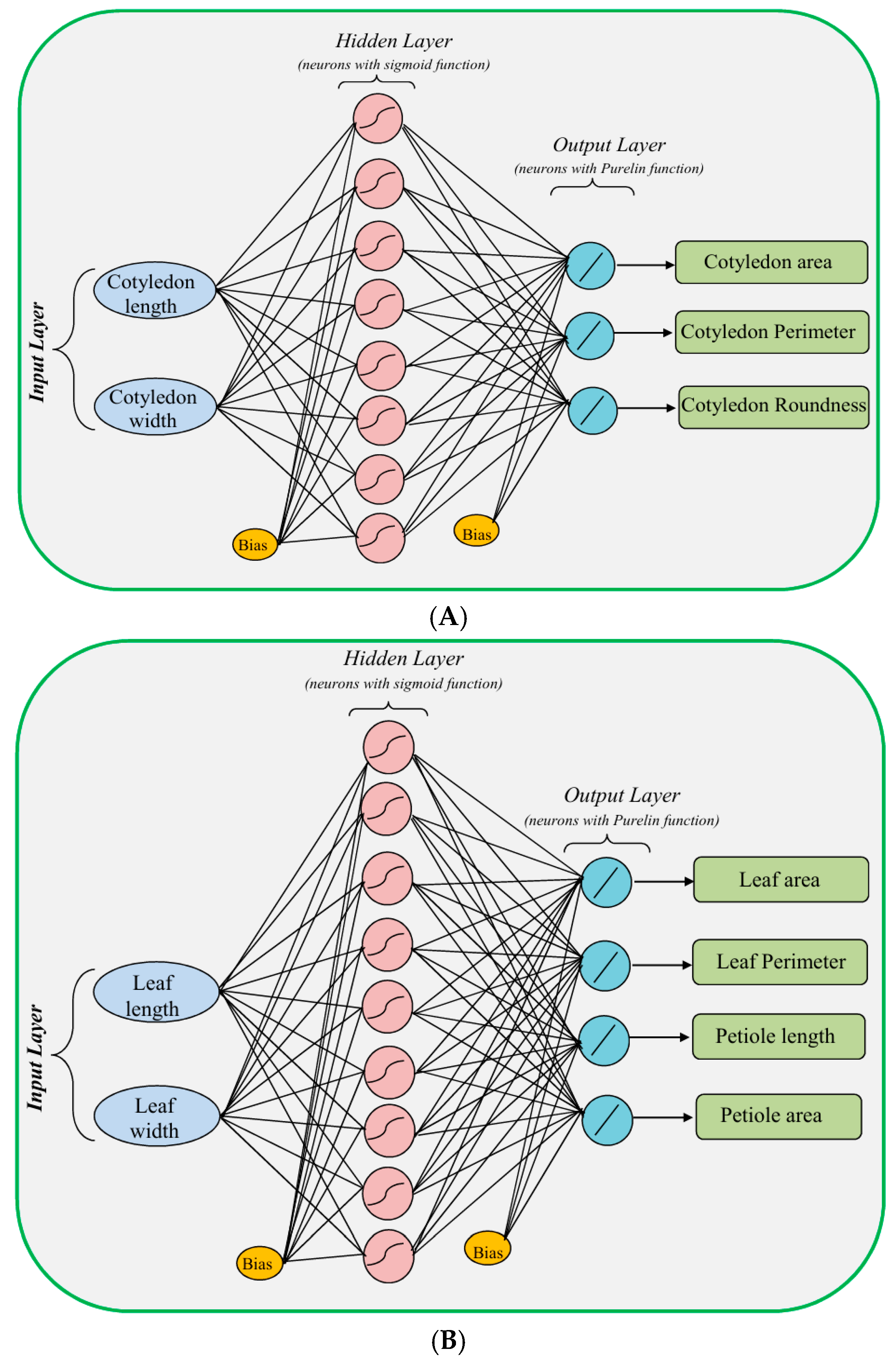
The best-fit ANN topologies for cotyledon and leaf traits are presented schematically in Figure 4. Each network employed a single hidden layer with a sigmoid activation function and a linear (purelin) output layer, and hidden-layer sizes were selected empirically to minimize validation MSE and maximize R2. All reported input counts excluded the bias unit. For cotyledon, the best performance of ANN was obtained with a 2–8–3 topology (i.e., an input layer of two factors (L, W), a hidden layer of eight neurons (output of the trial-and-error process), and an output layer of three factors (area, perimeter, and roundness)) (Figure 4; Table 3). The minimum MSE value (indicating an accurate prediction of the outputs for both training and test sets) was obtained with 8 neurons in the hidden layer, while the best validation performance (0.099879) occurred at epoch 11 (Supplementary Figure S1). For leaf, the best performance of ANN was achieved with a 2–9–4 topology (i.e., an input layer of two factors (L, W), a hidden layer of nine neurons, and an output layer of four factors (LA, perimeter, petiole length, and petiole area)) (Figure 4; Table 3). In this case, the minimum MSE was obtained with 9 neurons in the hidden layer, while the best validation performance (1.9272) was achieved at epoch 16 (Supplementary Figure S2).
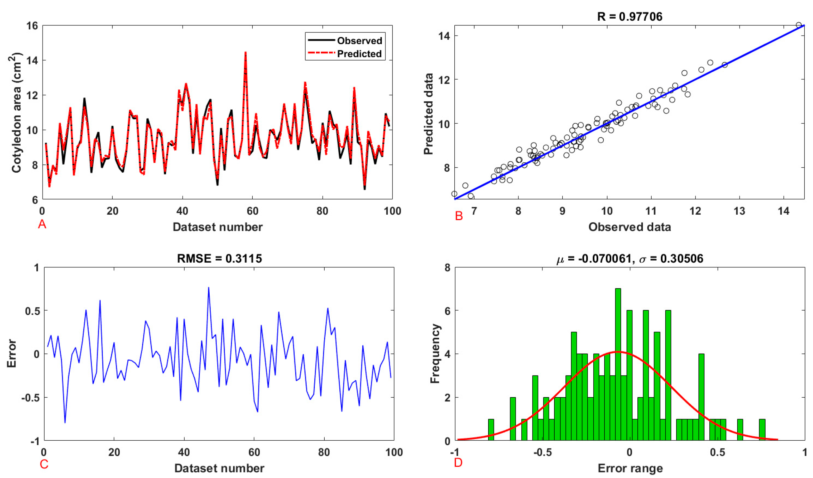
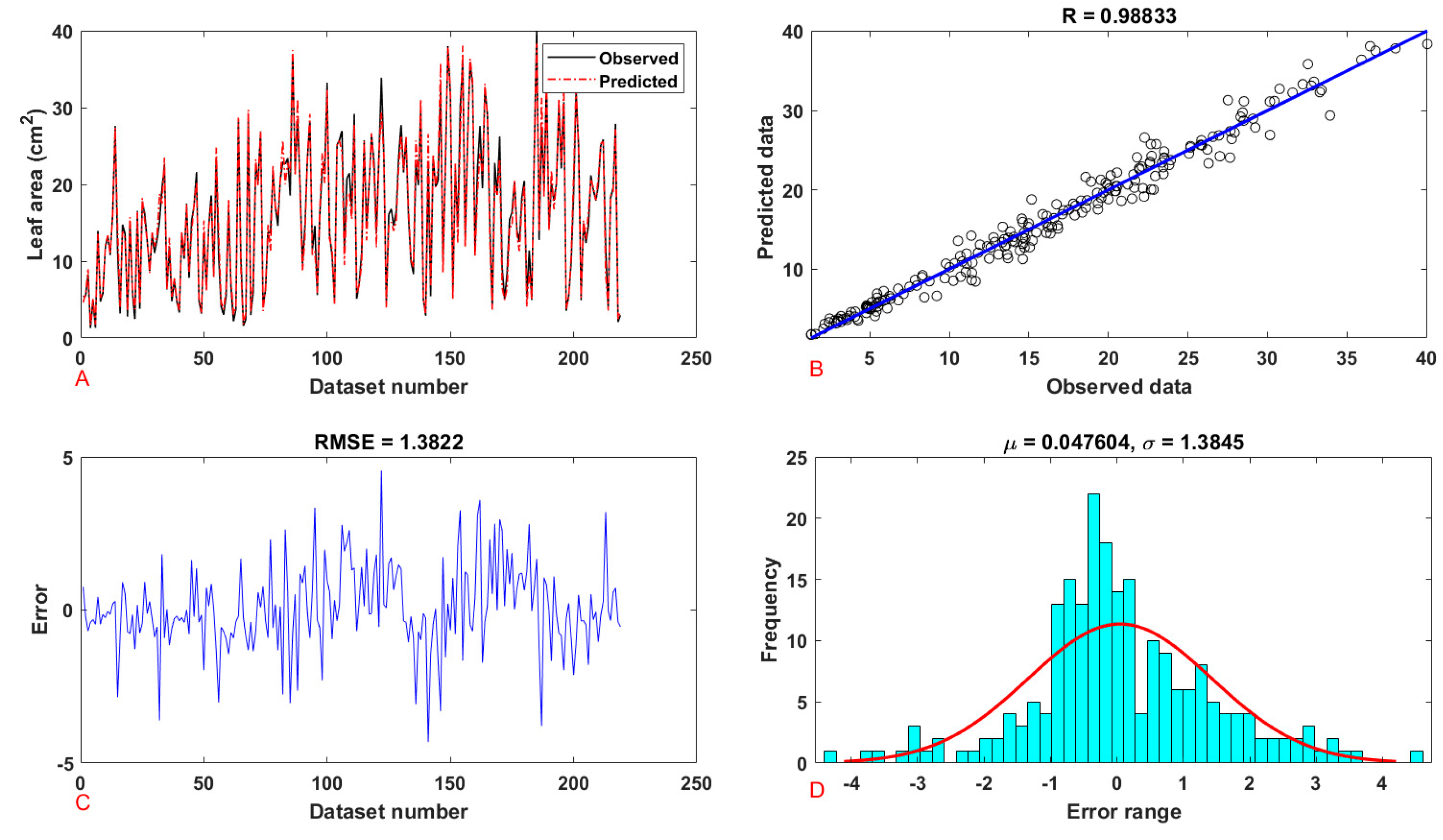
For both cotyledon and leaf, a high degree of agreement (concordance) between the ANN model-predicted and measured (actual) values was noted (Figure 5A and Figure 6A), indicating that the models are reliable and accurate in their predictions of cotyledon area and LA, respectively. When plotting the ANN model-predicted against the measured values, the data points lay in the vicinity of the 45° line (y = x), indicating high accuracy (Figure 5B and Figure 6B). The relative error (between the ANN model-predicted and measured data) was fairly consistent across the dataset (Figure 5C and Figure 6C), indicating that no specific ranges exist within the dataset where the model consistently overestimates or underestimates the measured values. In both organs, the distribution of errors (between the ANN model-predicted and measured data) was narrow and centered around zero (Figure 5D and Figure 6D), indicating high model accuracy. Additionally, all six employed statistical metrics indicated that the measured and (ANN) predicted values were very similar (e.g., R2 of 0.9546 and 0.9768, respectively; Table 4). Similar findings were noted for the remaining traits under study, including cotyledon perimeter (Supplementary Figure S3), cotyledon roundness (Supplementary Figure S4), leaf perimeter (Supplementary Figure S5), leaf petiole length (Supplementary Figure S6), and leaf petiole area (Supplementary Figure S7), where R2 values were 0.9136, 0.772, 0.8912, 0.9105, and 0.8696, respectively (Table 4). Taken together, these results indicate that the ANN models presented here provide very accurate estimates of cotyledon (area, perimeter, and roundness) and leaf (LA, perimeter, petiole length, and petiole area) traits.

3.3. Calculation of Whole-Seedling Area Based on Image-Derived Projected Area

Whole-seedling LA was closely related to seedling dry weight (R2 of 0.96). In this context, LA estimates can also serve as indicators of seedling dry weight.
Whole-seedling LA was computed based on projected area obtained from images captured at three different angles (side (0°; image plane parallel to the shoot), angle (45°), and top (90°; image plane parallel to growth medium surface); Figure 2). When considering a single view, the top one (90°) was associated with the highest accuracy in whole-seedling LA estimation, and the side view (0°) with the lowest (R2 of 0.88 and 0.73, respectively; Table 2). When considering two views, the accuracy of the whole-seedling LA estimation was always satisfactory (R2 ≥ 0.88), with the one combining the top and side views yielding the highest accuracy (R2 of 0.92). When considering three views, the accuracy of the whole-seedling LA estimation was not further improved compared with the combination of top and side views (R2 of 0.918 versus 0.920).
For validation of the whole-seedling LA models, their application was examined against a new independent dataset comprising 10 genotypes (8 cultivars and 2 traditional varieties; Supplementary Table S1). In all cases, the estimation accuracy was comparable to that reported above.
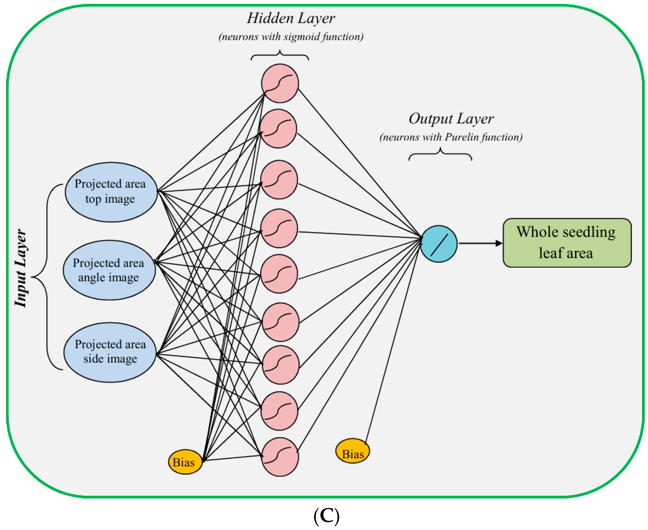
The best-fit ANN topology for whole-seedling LA is shown schematically in Figure 4 and follows the same configuration described above for organ traits (a single hidden layer with sigmoid activation, a linear output, and an empirically selected hidden-layer size). For whole-seedling scale, the ANN achieved its best performance with a 3–9–1 topology (i.e., an input layer of three factors (PAtop, PAside, PAangle), a hidden layer of nine neurons, and an output layer of one factor (whole-seedling LA)) (Figure 4; Table 3). The minimum MSE value was obtained with 9 neurons in the hidden layer, while the best validation performance (33.7232) occurred at epoch 33 (Supplementary Figure S8).
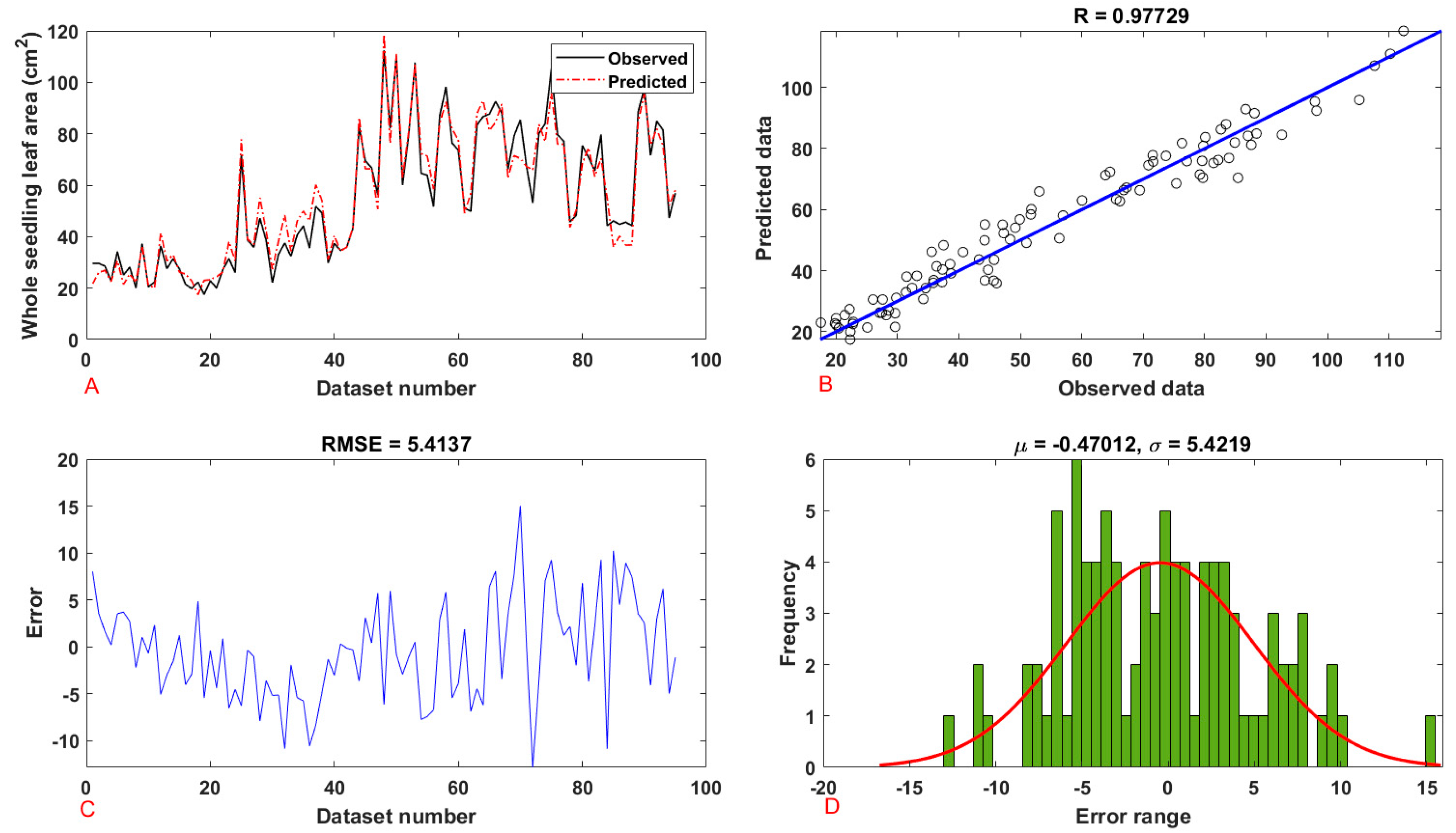
A high degree of agreement (concordance) between the ANN model-predicted and measured (actual) values was observed (Figure 7A), indicating that the model prediction of whole seedling area is both reliable and accurate. When plotting the ANN model-predicted against the measured values, the data points were centered near the 45° line (y = x), indicating high accuracy (Figure 7B). The relative error (between the ANN model-predicted and measured data) was fairly stable across the dataset (Figure 7C), indicating that no specific spans exist within the dataset where the model consistently overestimates or underestimates the measured values. Moreover, the distribution of errors (between the ANN model-predicted and measured data) was narrow and centered around zero (Figure 7D), indicating superior model accuracy. Eventually, all statistical metrics indicated that the measured and (ANN) predicted values were very close (e.g., R2 of 0.9551; Table 4).

3.4. Calculation of SPAD Value at Either Organ or Whole-Seedling Level

Cotyledon and leaf SPAD value were estimated from colorimetric features extracted from images at individual organ level (Figure 1). In all samples under evaluation, the magenta (M) color trait (CMYK color model) was zero, and therefore not considered further. Among the remaining 15 colorimetric features under study (Table 1), the yellow/blue value of the CIELAB color model (μb*) was the most effective for estimating cotyledon and leaf SPAD value (R2 of 0.771; Table 5). A more modest accuracy (0.662 ≤ R2 ≤ 0.736) was still achieved with another eight colorimetric features (μG, %B, μY, μK, μL, μH, μS, and μV). The remaining six colorimetric traits either gave an estimation with a lower accuracy (μR, %R; R2 of 0.605 and 0.581, respectively), or were not predictive of the SPAD value (μB, %G, μC, and μa*; R2 ≤ 0.488).
Whole-seedling SPAD value (average of all laminae) was also calculated from colorimetric features extracted from images at whole-seedling level (top view; Figure 2). Similarly to organ level, the magenta (M) color trait was zero, and therefore not examined further. Six colorimetric traits (μR, μG, %R, μK, μL, and μH) gave an estimation with a very low accuracy (0.415 ≤ R2 ≤ 0.439), while the remaining nine ones (μB, %G, %B, μC, μY, μa*, μb*, μS, and μV) were poor surrogates of the whole-seedling SPAD value (R2 ≤ 0.401; Table 5).
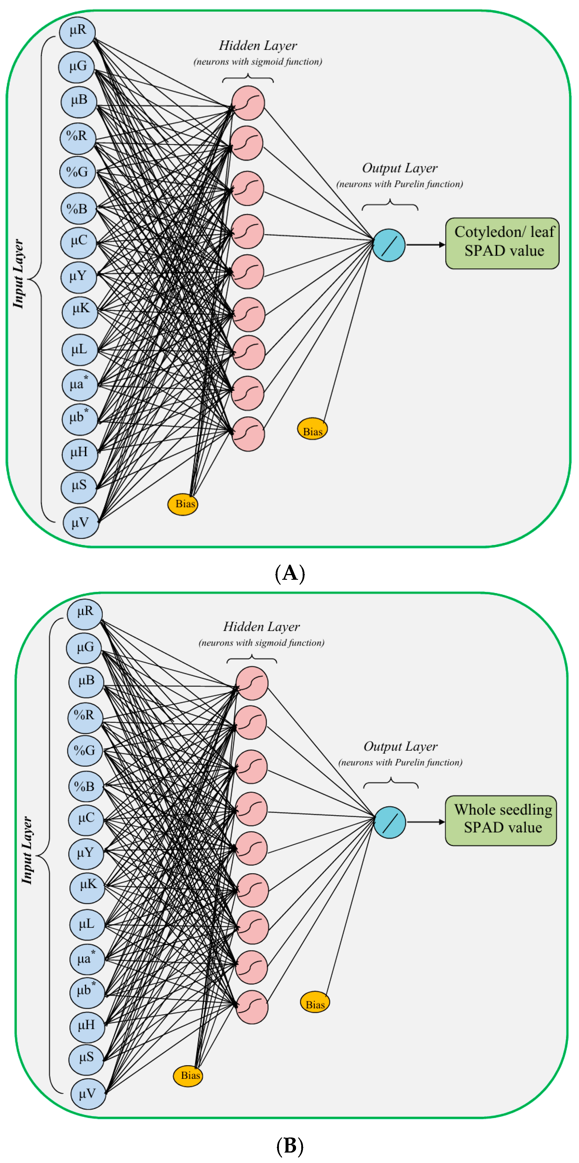
For cotyledon/leaf scale, the ANN achieved its best performance with a 15–9–1 topology (i.e., an input layer of 15 factors (all colorimetric features in Table 1 except magenta), a hidden layer of 9 neurons, and an output layer of 1 factor (SPAD value)) (Figure 8; Table 3). The minimum MSE value was obtained with 9 neurons in the hidden layer, while the best validation performance (5.58) occurred at epoch 26 (Supplementary Figure S9). For whole-seedling scale, the ANN achieved its best performance with a 15–9–1 topology (i.e., an input layer of 15 factors (all colorimetric features in Table 1 except magenta), a hidden layer of 9 neurons, and an output layer of 1 factor (SPAD value)) (Figure 8; Table 3). In this case, the minimum MSE was obtained with 9 neurons in the hidden layer, while the best validation performance (9.1315) was achieved at epoch 5 (Supplementary Figure S10).
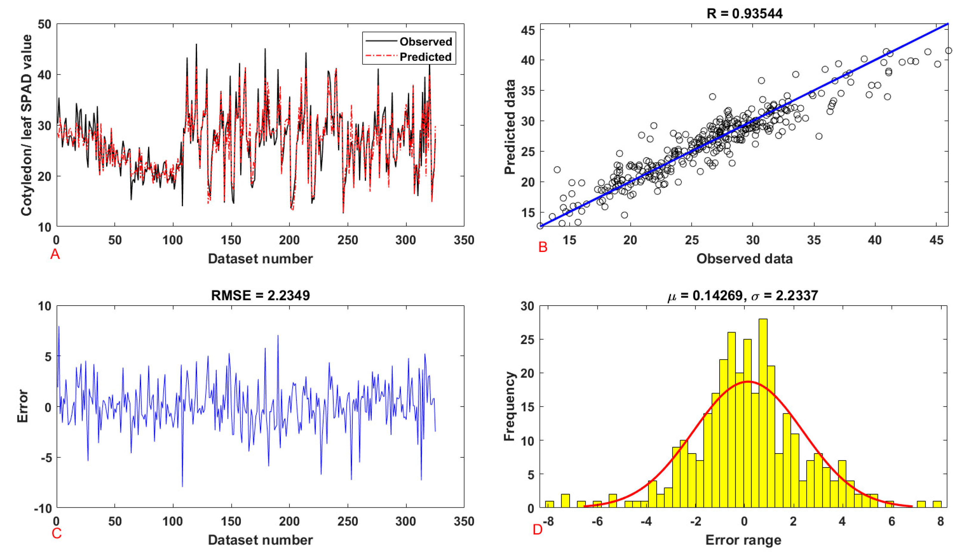
For the cotyledon/leaf scale, a high degree of agreement (concordance) between the ANN model-predicted and measured (actual) values was observed (Figure 9A), indicating reliable and accurate model predictions. At the plot of the ANN model-predicted versus the measured values, the data points lay around the 45° line (y = x), indicating high accuracy (Figure 9B). The relative error (between the ANN model-predicted and measured data) was also fairly stable across the dataset (Figure 9C), indicating that no areas exist within the dataset where the model consistently overestimates or underestimates the measured values. The distribution of errors (between the ANN model-predicted and measured data) was relatively narrow and centered around zero (Figure 9D), highlighting the increased model accuracy. Eventually, all six employed statistical metrics indicated that the measured and (ANN) predicted values were very close (e.g., R2 of 0.8751; Table 4).
For the whole-seedling scale, the model showed only modest accuracy, as evidenced by the degree of concordance between the ANN model-predicted and measured values (Figure 10A), the deviation from the 45° line (ANN model-predicted against the measured values; Figure 10B), the variation in the relative error across the dataset (Figure 10C), and the error density (Figure 10D), along with six statistical metrics (e.g., R2 of 0.5969; Table 4).

4. Discussion

4.1. Individual Cotyledon/Leaf Area Estimation by Employing Linear Dimensions

Evaluation of LA at the plant level lacks the level of detail, which is necessary to quantify the relative importance of different architectural elements of a given canopy [33]. For instance, determination of total LA cannot account for evaluations of the leaf size/number trade-off or the related effects on light interception [34,35]. In this perspective, area was firstly estimated at the individual organ (cotyledon, leaf) level. This task was undertaken by considering both conventional mathematical and ANN models.
A validated mathematical model for individual LA estimation based on leaf dimensions (L, W) is presented here for cucumber (R2 of 0.976; Table 2). Previously conducted studies devoted to mathematical prediction models are mostly limited to fully expanded leaves [8,9], which are highly relevant for adult plants. Provided that seedlings typically include a combination of expanding and fully expanded leaves [5,13], both states were considered for the model development in the present study. Additionally, another mathematical model was developed for cotyledon (R2 of 0.92; Table 2), which, to the authors’ knowledge, has not previously been studied, though may account for a considerable component of the whole-seedling area especially in the early phase [13].
Earlier leaf-dimension-based models estimating LA were generally robust to variations in cultivation conditions in two taxa (salinity level (Lycopersicon esculentum Mill. [36]) and irrigation regime (Olea europaea L. [12])), whereas adjustments in the model were required in a single species (altitudinal transect differences (Saussurea stoliczkai Clarke [37])). In order to fortify and broaden the applicability of the developed area estimation models, the employed material was cultivated under naturally fluctuating conditions, while three stress treatments (suboptimal temperature, salinity, and flooding) were also included. Additionally, the developed mathematical models were validated using a set of 10 cucumber genotypes (8 cultivars and 2 traditional varieties), which were obtained from different commercial sites. In this perspective, the derived prediction models were developed by considering environmentally induced differences in organ size and shape, and validated against phenotypic variation in these features arising from the interaction of genetic and cultivation factors.
By evaluating ANN models of various structures, the most effective network topology was identified for cotyledon and leaf area estimation (2–8–3 and 2–9–4, respectively; Figure 4; Table 3). Aligned with our expectations, the accuracy of estimation was superior when using ANN compared with conventional mathematical models (Table 2 and Table 4). ANN-based models for LA estimation have been previously developed for leaves of other species [24,38,39], whereas cotyledons have not been previously considered. To the best of our knowledge, this is the first report in which additional organ features (cotyledon (perimeter, roundness), leaf (perimeter, petiole length, petiole area)) were included as model outputs. The results of this study show that key shape aspects can be estimated with greater accuracy (R2 > 0.88; Table 4) by simply using L and W. Under the proposed initiative, information on shape traits is now readily available, which is regrettably absent from the relevant literature [7].
By using L and W as inputs, accurate estimations of area and specific shape traits were obtained for cotyledons and leaves. However, because the present study focused on seedlings, it remains unknown whether the retrieval of these shape traits is also valid for adult plants. Incorporating additional inputs, such as leaf thickness measured with a digital caliper, could provide an expanded array of architectural or morphometric features (e.g., leaf volume, specific leaf area, thickness-to-area ratio), thereby further broadening the applicability of cotyledon/leaf-level models. Future work may be directed toward these areas.
Although petiole is inherently a leaf component [7,40], its L is conventionally not included in leaf L in the relevant literature [8,9,33,41,42]. In this study, leaf L was defined as the sum of the petiole and lamina lengths (Figure 1). Notably, information on petiole area is essentially absent from previous studies devoted to LA estimation. Considering that petiole L was a significant component of leaf L (31%; range of 12.4–45.5%; Supplementary Table S2), though it marginally contributed to LA (4.2%; range of 1.49–12.5%; Supplementary Table S2), it was hypothesized that lamina L (in place of leaf L) would improve the accuracy of LA estimation. However, this hypothesis was not validated, as minor differences in the accuracy of LA estimation were apparent when considering lamina L instead of leaf L (Table 2). In this regard, LA can be accurately estimated using either lamina or leaf L in cucumber. This outcome is in accordance with earlier work on Chrysanthemum morifolium L. [7].
In scenarios where an unfeasibly high number of evaluations is required or measurement capacity is limited, area estimation via mathematical models may be based on a single organ dimension, albeit at the cost of reduced accuracy [7]. Compared with W, the model considering L was associated with higher accuracy in predicting area in both cotyledon and leaf (Table 2). In leaves, the superiority of L in area estimation has also been documented in some species (Vitis vinifera L. [41], O. europaea L. [12], Chr. morifolium L. [7]), whereas in others a better accuracy was evident for W (L. esculentum Mill. [36], Ribes grossularia L., Ribes rubrum L., Rubus fruticosus L., Rubus idaeus L., Vaccinium corymbosum L. [42]; Malus domestica Borch. [43]). The present results and those of earlier studies suggest that the selection of a single dimension for area prediction is species-specific and is a justifiable approach when the number of involved evaluations becomes a barrier.

4.2. Whole-Seedling LA Estimation by Employing the Projected Area

LA is widely recognized as the most important indicator of seedling quality [5,6]. LA determination conventionally relies on manual destructive approaches. The next step in technology entails digital image analysis, raising the possibility of non-invasive evaluations of a large number of samples over time [4,14]. With this methodology, LA is estimated based on the projected area (the 2D area of a 3D object projected onto a plane) [14]. The relation between LA and projected area depends on the shoot architecture, and is, thus, species-specific [4]. A few species have been earlier considered, thereby highlighting the need to develop respective databases for major horticultural crops.
By employing the projected area, the accuracy of whole-seedling LA estimation varied depending on the view angle (Table 2). The top view (90°) was associated with the highest accuracy (R2 of 0.88), whereas the side one (0°) with the lowest (R2 of 0.73; Table 2). In rice, instead, the side view was reported to provide more accurate LA estimations than the top one [44]. The accuracy of single-view LA estimation is compromised by image occlusions, namely, overlapping plant portions (thus not visible at a given angle), which may be alleviated by considering multiple view angles [4]. By combining any two views, the accuracy of the whole-seedling LA estimation was indeed satisfactory (R2 ≥ 0.88). By combining the top and side ones, the highest accuracy (R2 of 0.92) was noted. Although individual view data were not presented, Nagel et al. [45] also pointed out that considering both top and side views yielded accurate estimation of LA in barley and maize plants.
When considering all three views, no further improvement in the estimation accuracy was noted compared with combined top and side views (R2 of 0.918 versus 0.920; Table 2). As a next step and for the first time, ANN models were further employed for whole-seedling LA estimation (Figure 4; Table 3). Compared with conventional ones, the accuracy of estimation was improved. The developed ANN model allowed a very accurate quantification of whole-seedling LA (R2 of 0.955; Table 4). This study presents a screening protocol aligned with the data analysis pipeline which was experimentally verified for cucumber seedlings exposed to a range of conditions, and validated against 10 diverse cucumber genotypes (Supplementary Table S1) cultivated at different sites. This low-cost phenotyping option can either support scientists to address research needs or the horticultural industry to fill an unmet need for automation of seedling screening processes.
Although very accurate whole-seedling LA estimates were obtained in the present study, several limitations remain. As plant size increases and self-shading intensifies, occlusion becomes more pronounced and the accuracy of projected-area-based estimation is likely to decline [4]. Determining the plant size at which this effect becomes critical would be valuable. In addition, it is unclear whether this loss of accuracy is driven solely by plant size or whether other architectural traits (e.g., internode length, leaf length, leaf angle) also contribute, and, if so, to quantify their relative influence. Furthermore, the present work focused exclusively on leaf area, whereas other seedling-quality traits (e.g., compactness, height) were not examined. Future research could identify the stage at which occlusion begins to compromise accuracy, quantify the rate of this decline, and extend the approach to include additional morphometric indicators of seedling quality.

4.3. Cotyledon/Leaf, and Whole-Seedling SPAD Value Estimation by Employing Colorimetric Traits

Leaf greenness reflects chlorophyll content and serves as a reliable indicator of plant health and stress levels [4,16,17]. Chlorophyll content can be determined non-invasively using chlorophyll meters [17,18]. However, because of the small measuring area (approximately 2 × 3 mm), multiple within-leaf measurements are required [16], and the contact mode may cause damage to soft or fragile leaves (such as developing ones). To minimize the effects of chloroplast movement on chlorophyll meter readings, it is advisable to take measurements within a limited time window [18]. At seedling level, several leaves should be assessed to obtain representative and reliable results.
In this study, it was noted that organ (cotyledon and leaf) SPAD value can be accurately estimated (R2 of 0.771) by considering specific colorimetric features (yellow/blue value of the CIELAB color model (μb*)) extracted from RBG images (Table 2). It is indeed striking that the yellow/blue component (μb*) better represents organ SPAD value, whereas the red/green one (a*) seems irrelevant. Similarly to the present results, leaf SPAD values were strongly related to the blue color component in rice [21], whereas the strongest relationship was found with the green component in soybean [20]. Differences among species in leaf characteristics, along with variations between studies in image acquisition methods (e.g., sensor type, illumination conditions), may account for discrepancies in which color component shows the strongest relationship with SPAD values [22]. By employing an ANN model with a 15–9–1 topology (Figure 8; Table 3), the accuracy of organ (cotyledon and leaf) SPAD value was considerably improved (e.g., R2 of 0.8751; Table 4). In conclusion, the developed ANN model may be employed to measure organ (cotyledon and leaf) chlorophyll content within the workflow of a typical horticultural facility, serving as a decision-making tool to optimize cultivation practices such as nutrient and water management.
Although obtaining RBG images substantially reduces costs compared with other approaches (e.g., SPAD meters, hyperspectral imaging), the proposed toolkit depends on both precise organ positioning relative to the camera and consistent illumination conditions [27]. In this context, the proposed method is likely to be most applicable in controlled-light settings. This bottleneck could be overcome by acquiring organ images with a scanner [27].
Next, colorimetric features extracted from images at whole-seedling level (top view; Figure 2) were examined in parallel with the whole-seedling SPAD value (average of all laminae; Table 1). Using conventional models, colorimetric traits showed weak relationships with the whole-seedling SPAD value (R2 ≤ 0.439; Table 5). Using an ANN model (topology of 15–9–1; Figure 8; Table 3) considerably improved the estimation accuracy of the whole-seedling SPAD value, although it remained relatively modest (R2 of 0.597; Table 4). The heterogeneous nature of expanding and fully expanded leaves in combination with the 3D morphology of a seedling (e.g., variation in leaf petiole lengths (Supplementary Table S2) and inclination angles [34]) most likely limits the accuracy of whole-seedling SPAD value derived from 2D image-extracted colorimetric features.
Despite the relatively modest accuracy, the results obtained are encouraging and represent a potential new approach of using 2D image-extracted colorimetric features to gather information at the seedling level. Although advanced, complex methodologies of plant SPAD value estimation are currently in development (e.g., multi-spectral 3D imaging [46]), the framework under study clearly stands out for its simplicity, user-friendliness, and applicability. Although further improvement is warranted, the proposed model shows strong potential for supporting cost-effective monitoring strategies of plant health and stress level in the horticultural sector.
Potential ways to alleviate the noted limitations in whole-seedling SPAD value estimation include acquiring multiple views (i.e., not restricted to the top view as performed here) to compensate for leaf inclination and overlap. To minimize shading and within-seedling light heterogeneity, imaging should be performed under standardized conditions in enclosed, uniformly illuminated cabinets, or with diffuse, multi-directional LED lighting designed to achieve high spatial uniformity and reduce cast shadows. An additional step is the application of software-based color calibration, which typically involves including a reference target (e.g., a gray or color card) in each image or using built-in calibration algorithms so that all pixel values in the seedling image are adjusted relative to the reference [47]. This provides an extra layer of correction beyond the standardized imaging conditions, compensating for any residual variation in lighting or camera white balance and ensuring that color values remain comparable across the whole seedling surface. As a result of combining multiple viewing angles with a homogeneous lighting environment and software-based color calibration, colorimetric feature extraction becomes more representative of the whole seedling and may thereby enable more accurate estimation of whole-seedling SPAD values. These approaches may be explored in future work.

5. Conclusions

In cucumber, screening protocols and data analysis pipelines were established for area and SPAD value evaluation at both individual organ (cotyledon, leaf) and whole-seedling scales. By using length and width, individual organ area was precisely predicted (R2 ≥ 0.92). Based on image-extracted colorimetric features, individual-organ SPAD value was accurately retrieved (R2 of 0.77). By employing the 2D image-extracted projected areas obtained any combination of two angles (0°, 45°, and 90°), whole-seedling LA estimation was fairly feasible (R2 ≥ 0.88). In the above-mentioned case scenarios, the deployment of ANNs improved the estimation accuracy. Notably, ANNs additionally provided shape information of individual organs, and a reasonable approximation of the whole-seedling SPAD value (R2 of 0.597). Despite the uncertainty in the latter, the obtained outcome may be of particular benefit when remote (non-contact) monitoring is essential (e.g., fragile herbal material). For nursery managers and seedling producers, the proposed approach offers a rapid, low-cost, and non-destructive means to monitor seedling quality traits at scale, reducing labor requirements and enabling earlier detection of suboptimal growth or stress. Technically, the presented toolkit eases the analysis of key seedling features, encompassing overall quality. Importantly, the approach highlights both the potential and the current limitations (e.g., the expected reduced accuracy at larger plant sizes and for whole-seedling SPAD estimation), thereby guiding future research towards multi-angle imaging, improved color calibration, and the inclusion of additional morphometric inputs such as leaf thickness. By integrating these enhancements, the proposed methodology could be extended beyond the seedling stage and more readily adapted for high-throughput phenotyping or remote monitoring in commercial production systems.

Supplementary Materials

The following supporting information can be downloaded at: https://www.mdpi.com/article/10.3390/agronomy15102294/s1, Figure S1: Best validation performance in artificial neural networks (ANNs) model for cotyledon traits (model in Figure 4; traits in Figure 1); Figure S2: Best validation performance in artificial neural networks (ANNs) model for leaf traits (model in Figure 4; traits in Figure 1); Figure S3: Plots of testing dataset for artificial neural network (ANN) model performance to predict the cotyledon perimeter: A, the concordance plot with the results of ANN model along with the measured data; B, scatter plot of ANN-predicted versus measured values where the circles represent individual data points and the blue line represents the 1:1 (perfect-agreement) line; C, the relative error changes between the predicted and measured data; D, histogram of error density where the bars represent the frequency histogram of the errors and the red curve represents the fitted normal (Gaussian) distribution of those errors; Figure S4: Plots of testing dataset for artificial neural network (ANN) model performance to predict the cotyledon roundness: A, the concordance plot with the results of ANN model along with the measured data; B, scatter plot of ANN-predicted versus measured values where the circles represent individual data points and the blue line represents the 1:1 (perfect-agreement) line; C, the relative error changes between the predicted and measured data; D, histogram of error density where the bars represent the frequency histogram of the errors and the red curve represents the fitted normal (Gaussian) distribution of those errors; Figure S5: Plots of testing dataset for artificial neural network (ANN) model performance to predict the leaf perimeter: A, the concordance plot with the results of ANN model along with the measured data; B, scatter plot of ANN-predicted versus measured values where the circles represent individual data points and the blue line represents the 1:1 (perfect-agreement) line; C, the relative error changes between the predicted and measured data; D, histogram of error density where the bars represent the frequency histogram of the errors and the red curve represents the fitted normal (Gaussian) distribution of those errors; Figure S6: Plots of testing dataset for artificial neural network (ANN) model performance to predict the leaf petiole length: A, the concordance plot with the results of ANN model along with the measured data; B, scatter plot of ANN-predicted versus measured values where the circles represent individual data points and the blue line represents the 1:1 (perfect-agreement) line; C, the relative error changes between the predicted and measured data; D, histogram of error density where the bars represent the frequency histogram of the errors and the red curve represents the fitted normal (Gaussian) distribution of those errors; Figure S7: Plots of testing dataset for artificial neural network (ANN) model performance to predict the leaf petiole area: A, the concordance plot with the results of ANN model along with the measured data; B, scatter plot of ANN-predicted versus measured values where the circles represent individual data points and the blue line represents the 1:1 (perfect-agreement) line; C, the relative error changes between the predicted and measured data; D, histogram of error density where the bars represent the frequency histogram of the errors and the red curve represents the fitted normal (Gaussian) distribution of those errors; Figure S8: Best validation performance in artificial neural networks (ANNs) model for whole-seedling leaf area (model in Figure 4; traits in Figure 2); Figure S9: Best validation performance in artificial neural networks (ANNs) model for leaf/ cotyledon SPAD value (model in Figure 8); Figure S10: Best validation performance in artificial neural networks (ANNs) model for whole-seedling SPAD value (model in Figure 8); Table S1: Genetic variation in cotyledon and leaf shape traits of the 10 cucumber genotypes utilized for the individual organ and whole-seedling area estimation mathematical model validation. Means (±SE) followed by different letters within each row indicate significant differences based on Tukey’s honest significant difference test at p ≤ 0.05. For each cultivar, 10 cotyledons and at least 30 leaves were sampled (2–4 leaves/seedling); Table S2: The range of variation in the traits under study. For these traits, 630 cotyledons, 1450 leaves and 630 seedlings were considered; Table S3: Fitted coefficient (b) and constant (a) values of the regression models used to estimate petiole area (Ap) from leaf length (L), and petiole length (Lpetiole) measurements (Figure 1). For this analysis, 1450 leaves (encompassing different developmental stages) were considered.

Author Contributions

G.T.: Investigation, methodology, supervision, writing—review and editing, project administration, resources. T.M.: Investigation, methodology, data curation, formal analysis, visualization, writing—review and editing. D.P.: Data curation, mathematical model development, review and editing. N.N.: Data curation, formal analysis, visualization, review and editing. A.T.-G.: Data curation, artificial neural networks model development, visualization, review and editing. D.F.: Conceptualization, investigation, methodology, data curation, validation, visualization, supervision, writing—original draft, review, and editing. All authors have read and agreed to the published version of the manuscript.

Funding

This research received no external funding.

Data Availability Statement

The original contributions presented in this study are included in the article/Supplementary Material. Further inquiries can be directed to the corresponding author(s).

Acknowledgments

We are grateful to the students Sotiria Stavrakaki, Maria Skoubaki, Eleni Fylladitaki, Nikolaos Farsaris, and Georgios Filliandas for their valuable contributions in conducting the measurements. The seeds of two traditional varieties (Knossos, Gortyna) were produced with the financial support of Region of Crete. The authors also wish to thank Christos Lavdas (Rijk Zwaan, De Lier, The Netherlands) for the donation of the seed material (cv. ‘Aisopos’). We are grateful to the three reviewers for their careful evaluation and thoughtful recommendations, which have improved the final version of this paper.

Conflicts of Interest

The authors declare that they have no known competing financial interests or personal relationships that could have appeared to influence the work reported in this paper.

Abbreviations

a*, red/green; ANN, artificial neural network; B, blue; b*, yellow/blue; C, cyan; G, green; H, hue; K, black; L, length; L*, lightness; LA, leaf area; Lp, petiole length; M, magenta; MAE, mean absolute error; MLP, Multi-Layer-Perceptron; MSE, mean square error; PA, projected area; R, red; R, correlation coefficient; R2, coefficient of determination; RMSE, root mean square error; RSNNS, R Stuttgart Neural Network Simulator; S, saturation; SEP, standard error of prediction; V, value; W, width; Y, yellow.

References

  1. Gallegos-Cedillo, V.M.; Nájera, C.; Gruda, N.S.; Signore, A.; Gallegos, J.; Rodríguez, R.; Ochoa, J.; Egea-Gilabert, C.; Fernández, J.A. An In-Depth Analysis of Sustainable Practices in Vegetable Seedlings Nurseries: A Review. Sci. Hortic. 2024, 334, 113342. [Google Scholar] [CrossRef]
  2. Gallegos-Cedillo, V.M.; Nájera, C.; Signore, A.; Ochoa, J.; Gallegos, J.; Egea-Gilabert, C.; Gruda, N.S.; Fernández, J.A. Analysis of Global Research on Vegetable Seedlings and Transplants and Their Impacts on Product Quality. J. Sci. Food Agric. 2024, 104, 4950–4965. [Google Scholar] [CrossRef] [PubMed]
  3. He, J.; Ning, K.; Naznin, A.; Wang, Y.; Chen, C.; Zuo, Y.; Zhou, M.; Li, C.; Varshney, R.; Chen, Z.-H. Technological Advances in Imaging and Modelling of Leaf Structural Traits: A Review of Heat Stress in Wheat. J. Exp. Bot. 2025, eraf070. [Google Scholar] [CrossRef]
  4. Zhang, H.; Wang, L.; Jin, X.; Bian, L.; Ge, Y. High-Throughput Phenotyping of Plant Leaf Morphological, Physiological, and Biochemical Traits on Multiple Scales Using Optical Sensing. Crop J. 2023, 11, 1303–1318. [Google Scholar] [CrossRef]
  5. Moosavi-Nezhad, M.; Salehi, R.; Aliniaeifard, S.; Tsaniklidis, G.; Woltering, E.J.; Fanourakis, D.; Żuk-Gołaszewska, K.; Kalaji, H.M. Blue Light Improves Photosynthetic Performance during Healing and Acclimatization of Grafted Watermelon Seedlings. Int. J. Mol. Sci. 2021, 22, 8043. [Google Scholar] [CrossRef] [PubMed]
  6. Li, C.; Adhikari, R.; Yao, Y.; Miller, A.G.; Kalbaugh, K.; Li, D.; Nemali, K. Measuring Plant Growth Characteristics Using Smartphone Based Image Analysis Technique in Controlled Environment Agriculture. Comput. Electron. Agric. 2020, 168, 105123. [Google Scholar] [CrossRef]
  7. Fanourakis, D.; Kazakos, F.; Nektarios, P.A. Allometric Individual Leaf Area Estimation in Chrysanthemum. Agronomy 2021, 11, 795. [Google Scholar] [CrossRef]
  8. Cho, Y.Y.; Oh, S.; Oh, M.M.; Son, J.E. Estimation of Individual Leaf Area, Fresh Weight, and Dry Weight of Hydroponically Grown Cucumbers (Cucumis sativus L.) Using Leaf Length, Width, and SPAD Value. Sci. Hortic. 2007, 111, 330–334. [Google Scholar] [CrossRef]
  9. Blanco, F.F.; Folegatti, M.V. Estimation of Leaf Area for Greenhouse Cucumber by Linear Measurements under Salinity and Grafting. Sci. Agric. 2005, 62, 305–309. [Google Scholar] [CrossRef]
  10. Huaccha-Castillo, A.E.; Fernandez-Zarate, F.H.; Pérez-Delgado, L.J.; Tantalean-Osores, K.S.; Vaca-Marquina, S.P.; Sanchez-Santillan, T.; Morales-Rojas, E.; Seminario-Cunya, A.; Quiñones-Huatangari, L. Non-Destructive Estimation of Leaf Area and Leaf Weight of Cinchona officinalis L. (Rubiaceae) Based on Linear Models. For. Sci. Technol. 2023, 19, 59–67. [Google Scholar] [CrossRef]
  11. Gao, M.; Van der Heijden, G.W.A.M.; Vos, J.; Eveleens, B.A.; Marcelis, L.F.M. Estimation of Leaf Area for Large Scale Phenotyping and Modeling of Rose Genotypes. Sci. Hortic. 2012, 138, 227–234. [Google Scholar] [CrossRef]
  12. Koubouris, G.; Bouranis, D.; Vogiatzis, E.; Nejad, A.R.; Giday, H.; Tsaniklidis, G.; Ligoxigakis, E.K.; Blazakis, K.; Kalaitzis, P.; Fanourakis, D. Leaf Area Estimation by Considering Leaf Dimensions in Olive Tree. Sci. Hortic. 2018, 240, 440–445. [Google Scholar] [CrossRef]
  13. Hayashi, E.; Amagai, Y.; Kozai, T.; Maruo, T.; Tsukagoshi, S.; Nakano, A.; Johkan, M. Variations in the Growth of Cotyledons and Initial True Leaves as Affected by Photosynthetic Photon Flux Density at Individual Seedlings and Nutrients. Agronomy 2022, 12, 194. [Google Scholar] [CrossRef]
  14. Poorter, H.; Hummel, G.M.; Nagel, K.A.; Fiorani, F.; von Gillhaussen, P.; Virnich, O.; Schurr, U.; Postma, J.A.; van de Zedde, R.; Wiese-Klinkenberg, A. Pitfalls and Potential of High-Throughput Plant Phenotyping Platforms. Front. Plant Sci. 2023, 14, 1233794. [Google Scholar] [CrossRef]
  15. Li, D.; Li, C.; Yao, Y.; Li, M.; Liu, L. Modern Imaging Techniques in Plant Nutrition Analysis: A Review. Comput. Electron. Agric. 2020, 174, 105459. [Google Scholar] [CrossRef]
  16. Xiong, D.; Chen, J.; Yu, T.; Gao, W.; Ling, X.; Li, Y.; Peng, S.; Huang, J. SPAD-Based Leaf Nitrogen Estimation Is Impacted by Environmental Factors and Crop Leaf Characteristics. Sci. Rep. 2015, 5, 13389. [Google Scholar] [CrossRef]
  17. Padilla, F.M.; Peña-Fleitas, M.T.; Gallardo, M.; Giménez, C.; Thompson, R.B. Derivation of Sufficiency Values of a Chlorophyll Meter to Estimate Cucumber Nitrogen Status and Yield. Comput. Electron. Agric. 2017, 141, 54–64. [Google Scholar] [CrossRef]
  18. Hlavinka, J.; Nauš, J.; Špundová, M. Anthocyanin Contribution to Chlorophyll Meter Readings and Its Correction. Photosynth. Res. 2013, 118, 277–295. [Google Scholar] [CrossRef]
  19. Yang, H.; Li, J.; Yang, J.; Wang, H.; Zou, J.; He, J. Effects of Nitrogen Application Rate and Leaf Age on the Distribution Pattern of Leaf SPAD Readings in the Rice Canopy. PLoS ONE 2014, 9, e88421. [Google Scholar] [CrossRef]
  20. Rigon, J.P.G.; Capuani, S.; Fernandes, D.M.; Guimarães, T.M. A Novel Method for the Estimation of Soybean Chlorophyll Content Using a Smartphone and Image Analysis. Photosynthetica 2016, 54, 559–566. [Google Scholar] [CrossRef]
  21. Mohan, P.J.; Gupta, S.D. Intelligent Image Analysis for Retrieval of Leaf Chlorophyll Content of Rice from Digital Images of Smartphone under Natural Light. Photosynthetica 2019, 57, 388–398. [Google Scholar] [CrossRef]
  22. Peters, R.D.; Noble, S.D. Characterization of Leaf Surface Phenotypes Based on Light Interaction. Plant Methods 2023, 19, 26. [Google Scholar] [CrossRef] [PubMed]
  23. Taheri-Garavand, A.; Mumivand, H.; Fanourakis, D.; Fatahi, S.; Taghipour, S. An Artificial Neural Network Approach for Non-Invasive Estimation of Essential Oil Content and Composition through Considering Drying Processing Factors: A Case Study in Mentha aquatica. Ind. Crops Prod. 2021, 171, 113985. [Google Scholar] [CrossRef]
  24. Rahimikhoob, H.; Delshad, M.; Habibi, R. Leaf Area Estimation in Lettuce: Comparison of Artificial Intelligence-Based Methods with Image Analysis Technique. Measurement 2023, 222, 113636. [Google Scholar] [CrossRef]
  25. Nasiri, A.; Taheri-Garavand, A.; Fanourakis, D.; Zhang, Y.-D.; Nikoloudakis, N. Automated Grapevine Cultivar Identification via Leaf Imaging and Deep Convolutional Neural Networks: A Proof-of-Concept Study Employing Primary Iranian Varieties. Plants 2021, 10, 1628. [Google Scholar] [CrossRef]
  26. Fanourakis, D.; Papadakis, V.M.; Machado, M.; Psyllakis, E.; Nektarios, P.A. Non-invasive Leaf Hydration Status Determination through Convolutional Neural Networks Based on Multispectral Images in Chrysanthemum. Plant Growth Regul. 2024, 102, 485–496. [Google Scholar] [CrossRef]
  27. Taheri-Garavand, A.; Rezaei Nejad, A.; Fanourakis, D.; Fatahi, S.; Ahmadi Majd, M. Employment of Artificial Neural Networks for Non-Invasive Estimation of Leaf Water Status Using Color Features: A Case Study in Spathiphyllum wallisii. Acta Physiol. Plant 2021, 43, 78. [Google Scholar] [CrossRef]
  28. Gupta, S.; Rosenthal, D.M.; Stinchcombe, J.R.; Baucom, R.S. The Remarkable Morphological Diversity of Leaf Shape in Sweet Potato (Ipomoea batatas): The Influence of Genetics, Environment, and G × E. New Phytol. 2020, 225, 2183–2195. [Google Scholar] [CrossRef]
  29. Tjandra, A.D.; Heywood, T.; Chandrawati, R. Trigit: A Free Web Application for Rapid Colorimetric Analysis of Images. Biosens. Bioelectron. X 2023, 14, 100361. [Google Scholar] [CrossRef]
  30. Lhotáková, Z.; Neuwirthová, E.; Potůčková, M.; Červená, L.; Hunt, L.; Kupková, L.; Lukeš, P.; Campbell, P.; Albrechtová, J. Mind the Leaf Anatomy While Taking Ground Truth with Portable Chlorophyll Meters. Sci. Rep. 2025, 15, 1855. [Google Scholar] [CrossRef]
  31. Dai, W.; Hamasaki, T. Statistics in Medicine, 4th ed.; Riffenburgh, R.H., Gillen, D.L., Eds.; Academic Press: Oxford, UK, 2020; Volume 76. [Google Scholar]
  32. Hagan, M.T.; Demuth, H.B.; Beale, M. Neural Network Design; PWS Publishing Co.: Boston, MA, USA, 1996. [Google Scholar]
  33. Koyama, K.; Smith, D.D. Scaling the Leaf Length-Times-Width Equation to Predict Total Leaf Area of Shoots. Ann. Bot. 2022, 130, 215–230. [Google Scholar] [CrossRef]
  34. Qian, T.; Zheng, X.; Guo, X.; Wen, W.; Yang, J.; Lu, S. Influence of Temperature and Light Gradient on Leaf Arrangement and Geometry in Cucumber Canopies: Structural Phenotyping Analysis and Modelling. Inf. Process. Agric. 2019, 6, 224–232. [Google Scholar] [CrossRef]
  35. Huang, Y.; Lechowicz, M.J.; Price, C.A.; Li, L.; Wang, Y.; Zhou, D. The Underlying Basis for the Trade-off between Leaf Size and Leafing Intensity. Funct. Ecol. 2016, 30, 199–205. [Google Scholar] [CrossRef]
  36. Schwarz, D.; Kläring, H.-P. Allometry to Estimate Leaf Area of Tomato. J. Plant Nutr. 2001, 24, 1291–1309. [Google Scholar] [CrossRef]
  37. Wang, Z.; Zhang, L. Leaf Shape Alters the Coefficients of Leaf Area Estimation Models for Saussurea stoliczkai in Central Tibet. Photosynthetica 2012, 50, 337–342. [Google Scholar] [CrossRef]
  38. Kumar, M.K.; Kumar, R.S.; Sankar, V.; Sakthivel, T.; Karunakaran, G.; Tripathi, P. Non-Destructive Estimation of Leaf Area of Durian (Durio zibethinus)—An Artificial Neural Network Approach. Sci. Hortic. 2017, 219, 319–325. [Google Scholar]
  39. Cemek, B.; Ünlükara, A.; Kurunç, A.; Küçüktopcu, E. Leaf Area Modeling of Bell Pepper (Capsicum annuum L.) Grown under Different Stress Conditions by Soft Computing Approaches. Comput. Electron. Agric. 2020, 174, 105514. [Google Scholar] [CrossRef]
  40. Li, G.; Yang, D.; Sun, S. Allometric Relationships between Lamina Area, Lamina Mass and Petiole Mass of 93 Temperate Woody Species Vary with Leaf Habit, Leaf Form and Altitude. Funct. Ecol. 2008, 22, 557–564. [Google Scholar] [CrossRef]
  41. Montero, F.J.; de Juan, J.A.; Cuesta, A.; Brasa, A. Nondestructive Methods to Estimate Leaf Area in Vitis vinifera L. HortScience 2000, 35, 696–698. [Google Scholar] [CrossRef]
  42. Fallovo, C.; Cristofori, V.; Mendoza de-Gyves, E.; Rivera, C.M.; Rea, R.; Fanasca, S.; Bignami, C.; Sassine, Y.; Rouphael, Y. Leaf Area Estimation Model for Small Fruits from Linear Measurements. HortScience 2008, 43, 2263–2267. [Google Scholar] [CrossRef]
  43. Sala, F.; Arsene, G.-G.; Iordănescu, O.; Boldea, M. Leaf Area Constant Model in Optimizing Foliar Area Measurement in Plants: A Case Study in Apple Tree. Sci. Hortic. 2015, 193, 218–224. [Google Scholar] [CrossRef]
  44. Jiang, N.; Yang, W.; Duan, L.; Chen, G.; Fang, W.; Xiong, L.; Liu, Q. A Nondestructive Method for Estimating the Total Green Leaf Area of Individual Rice Plants Using Multi-Angle Color Images. J. Innov. Opt. Health Sci. 2015, 8, 1550002. [Google Scholar] [CrossRef]
  45. Nagel, K.A.; Putz, A.; Gilmer, F.; Heinz, K.; Fischbach, A.; Pfeifer, J.; Faget, M.; Blossfeld, S.; Ernst, M.; Dimaki, C.; et al. Growscreen-Rhizo Is a Novel Phenotyping Robot Enabling Simultaneous Measurements of Root and Shoot Growth for Plants Grown in Soil-Filled Rhizotrons. Funct. Plant Biol. 2012, 39, 891. [Google Scholar] [CrossRef] [PubMed]
  46. Sun, G.; Wang, X.; Sun, Y.; Ding, Y.; Lu, W. Measurement Method Based on Multispectral Three-Dimensional Imaging for the Chlorophyll Contents of Greenhouse Tomato Plants. Sensors 2019, 19, 3345. [Google Scholar] [CrossRef] [PubMed]
  47. Sunoj, S.; Igathinathane, C.; Saliendra, N.; Hendrickson, J.; Archer, D. Color Calibration of Digital Images for Agriculture and Other Applications. ISPRS J. Photogramm. Remote Sens. 2018, 146, 221–234. [Google Scholar] [CrossRef]
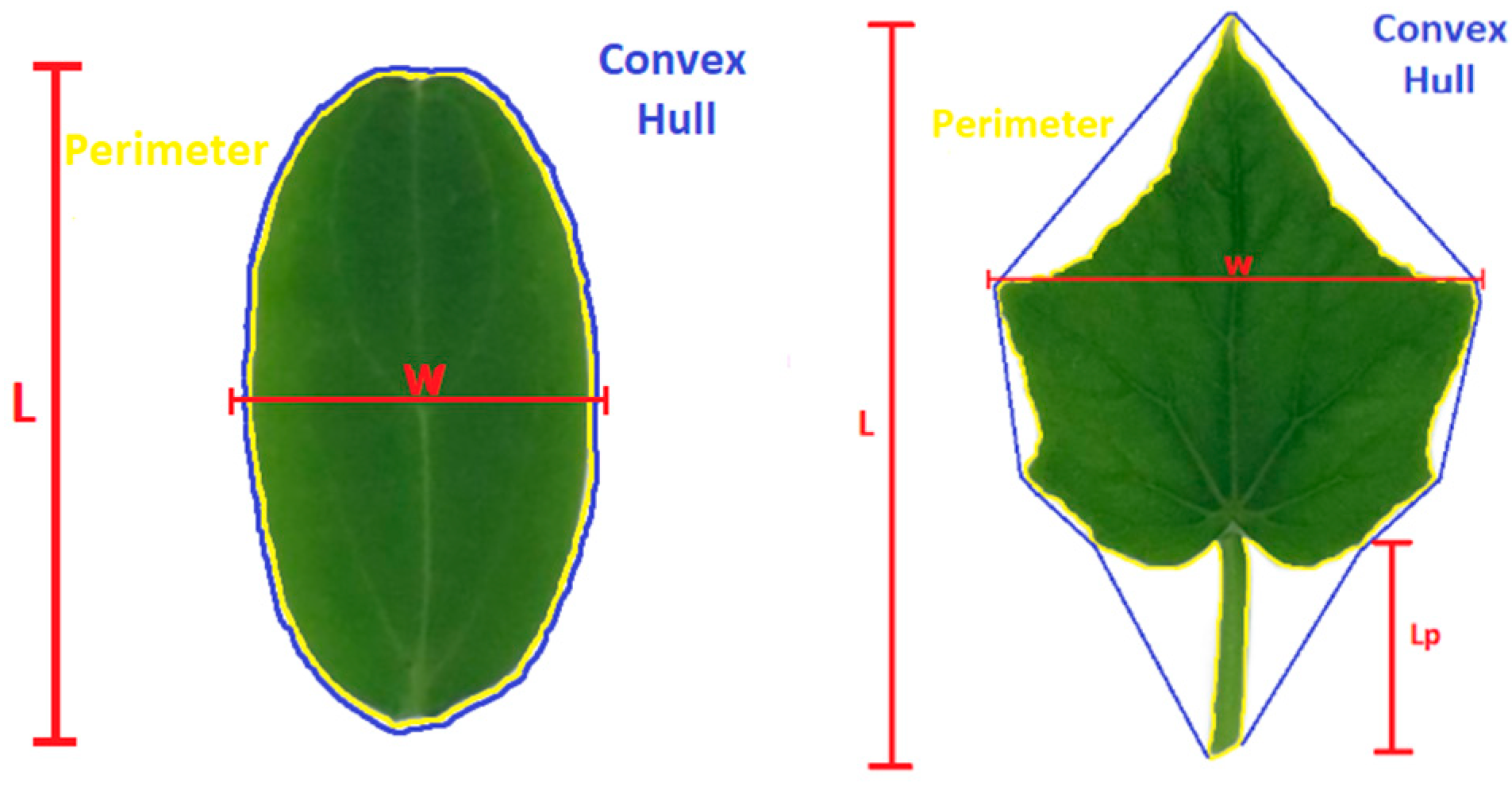
Figure 1. Examples of morphometric features recorded on a cucumber seedling cotyledon (left) and true leaf (right). Arrows indicate the linear dimensions measured (petiole length, Lp; cotyledon/leaf length, L; and cotyledon/leaf width, W), while the yellow line shows the organ perimeter and the blue line the convex-hull outline.
Agronomy 15 02294 g001
Figure 2. Representative images of the same cucumber seedling captured through the side (0°; image plane parallel to the shoot), angle (45°; intermediate between side and top), and top (90°; image plane parallel to growth medium surface) views (left, middle, and right image). Projected area from each view (0°, 45°, and 90°) was quantified with ImageJ, while the top-view image (90°) was additionally processed with Trigit to extract colorimetric features. Scale bar = 5 cm.
Agronomy 15 02294 g002
Figure 3. Flow chart of the artificial neural network (ANN) training and validation process used to estimate area and SPAD value at both organ and whole-seedling scales. The chart outlines the sequential steps followed in model development, including data import and normalization, division into training, validation and testing sets, selection of learning algorithm and network parameters (number of hidden layers, neurons, and transfer functions), network training, performance validation, iteration until acceptable error was reached, and final deployment of the trained ANN for prediction.
Agronomy 15 02294 g003
Figure 4. Best-fit artificial neural network (ANN) topologies developed for cucumber seedlings at the cotyledon, leaf, and whole-seedling levels. Panels show the network architectures used to predict (A) cotyledon traits, (B) leaf traits, and (C) whole-seedling leaf area, including the number of input variables, hidden-layer neurons, and output variables. These topologies achieved the lowest mean square error (MSE) and highest coefficients of determination (R2) during model validation.
Agronomy 15 02294 g004aAgronomy 15 02294 g004b
Figure 5. Performance of the artificial neural network (ANN) model in predicting cotyledon area. Plots show (A) concordance between measured and ANN-predicted values, (B) scatter plot of ANN-predicted versus measured values where the circles represent individual data points and the blue line represents the 1:1 (perfect-agreement) line, (C) relative error across the dataset, and (D) histogram of error density where the bars represent the frequency histogram of the errors and the red curve represents the fitted normal (Gaussian) distribution of those errors. These panels demonstrate the accuracy and distribution of prediction errors for the trained network.
Agronomy 15 02294 g005
Figure 6. Performance of the artificial neural network (ANN) model in predicting leaf area (individual leaves). Plots show (A) concordance between measured and ANN-predicted values, (B) scatter plot of ANN-predicted versus measured values where the circles represent individual data points and the blue line represents the 1:1 (perfect-agreement) line, (C) relative error across the dataset, and (D) histogram of error density where the bars represent the frequency histogram of the errors and the red curve represents the fitted normal (Gaussian) distribution of those errors. These panels illustrate the accuracy and distribution of prediction errors for the trained network.
Agronomy 15 02294 g006
Figure 7. Performance of the artificial neural network (ANN) model in predicting whole-seedling leaf area. Panels show (A) concordance between measured and ANN-predicted values, (B) scatter plot of ANN-predicted versus measured values where the circles represent individual data points and the blue line represents the 1:1 (perfect-agreement) line, (C) relative error across the dataset, and (D) histogram of error density where the bars represent the frequency histogram of the errors and the red curve represents the fitted normal (Gaussian) distribution of those errors. These plots illustrate the accuracy and distribution of prediction errors for the trained network.
Agronomy 15 02294 g007
Figure 8. Best-fit artificial neural network (ANN) topologies developed to estimate SPAD values of cucumber seedlings at different scales. Panels depict the network architectures used to predict (A) cotyledon/leaf SPAD value and (B) whole-seedling SPAD value, showing the number of input variables, hidden-layer neurons, and output variable. These topologies produced the lowest mean square error (MSE) and highest coefficients of determination (R2) during model validation.
Agronomy 15 02294 g008
Figure 9. Performance of the artificial neural network (ANN) model in predicting cotyledon/leaf SPAD value. Panels show (A) concordance between measured and ANN-predicted values, (B) scatter plot of ANN-predicted versus measured values where the circles represent individual data points and the blue line represents the 1:1 (perfect-agreement) line, (C) relative error across the dataset, and (D) histogram of error density where the bars represent the frequency histogram of the errors and the red curve represents the fitted normal (Gaussian) distribution of those errors. These plots illustrate the accuracy and distribution of prediction errors for the trained network.
Agronomy 15 02294 g009
Figure 10. Performance of the artificial neural network (ANN) model in predicting whole-seedling SPAD value. Panels show (A) concordance between measured and ANN-predicted values, (B) scatter plot of ANN-predicted versus measured values where the circles represent individual data points and the blue line represents the 1:1 (perfect-agreement) line, (C) relative error across the dataset, and (D) histogram of error density where the bars represent the frequency histogram of the errors and the red curve represents the fitted normal (Gaussian) distribution of those errors. These plots illustrate the accuracy and distribution of prediction errors for the trained network.
Agronomy 15 02294 g010
Table 1. Morphometric, colorimetric, and derived parameters assessed in cucumber seedlings at the cotyledon, leaf, and whole-seedling levels. The table lists the parameter name, description, level of assessment (organ or seedling), calculation formula, and range/unit. Dimension, area, and shape traits were derived from digital images using ImageJ, whereas color features were extracted with Trigit.
DescriptionLevelParameterFormulaRange (unit)
DimensionCotyledonLength (L) From base to top along middle vein (major axis)(cm)
LeafPetiole (stalk) L (Lp)From petiole base to leaf base
Lamina (blade) LFrom base to top along middle vein
Leaf LLp + lamina length (major axis)
Cotyledon/leafWidth (W)Widest point along the transverse axis perpendicular to the longitudinal one (minor axis)
PerimeterLength of the path enclosing the outline along the margins (edges)
AreaCotyledonCotyledon areaOne-sided planar surface area(cm2)
LeafPetiole area
Lamina area
Leaf area (LA)Petiole area + lamina area
Seedling 1Projected area (PA)Area of green pixels obtained by seedling image
ShapeCotyledon/leafAspect ratio m i n o r   a x i s m a j o r   a x i s 1–∞ (−)
Circularity 4 π × a r e a ( p e r i m e t e r ) 2 0–1 (−)
Roundness 4 × a r e a 4 π × ( m a j o r   a x i s ) 2 0–1 (−)
Solidity a r e a c o n v e x   a r e a 0–1 (−)
LeafLp to leaf L ratio L p l e a f   L × 100 0≤
<100 (%)
Petiole area to LA ratio p e t i o l e   a r e a L A × 100
ColorLeaf/seedling 2Red (R) 4amount of red0–255 (−)
Green (G) 4amount of green
Blue (B) 4amount of blue
%R R R + G + B × 100 0≤
≤100 (%)
%G G R + G + B × 100
%B B R + G + B × 100
Cyan (C) 5 0–100 (%)
Magenta (M) 5
Yellow (Y) 5
Black (K) 5
Lightness (L*) 60 specifies black, 100 specifies white
Red/green (a*) 6Amount of red or green tones −110–110 (−)
Yellow/blue (b*) 6Amount of yellow or blue tones
Hue (H) 7Location on the color wheel0–360 (°)
Saturation (S) 7Vividness or dullness 0–255 (−)
Value (V) 7Amount of white
ContentLeaf/seedling 3SPAD valueNon-invasive optical measurement of total chlorophyll content0–100 (−)
1 Seedling imaged from different views (side, angle, top); 2 seedling imaged from the top; 3 average of cotyledons and leaves; 4 RGB color model; 5 CMYK color model; 6 CIELAB color model; 7 HSV color model.
Table 2. Fitted coefficient (b) and constant (a) values of the regression models used to estimate the area of cotyledon, leaf, and whole seedling in cucumber. In single cotyledons, area (Ac) computation was based on length (L) and width (W) measurements (Figure 1). In single leaves, leaf area (LA) computation was based on leaf L, lamina length (Llamina), and leaf W measurements (Figure 1). Whole-seedling LA computation was based on projected area (PA) extracted by images acquired from different view angles (top, side, angle; Figure 2). For each model, the coefficient of determination (R2), mean square error (MSE), and 95% bootstrap confidence limits (BC lower/upper) are provided. For these analyses, 630 cotyledons, 1450 leaves (encompassing different developmental stages), and 630 seedlings (encompassing different developmental stages) were considered.
LevelModelb (Fitted Coefficient) a (Constant) R2 MSE BC LowerBC Upper
Cotyledon1Ac = a + b · L2.99−5.320.8330.340.8090.858
2Ac = a + b · L20.292.140.8400.320.8140.869
3Ac = a + b · L30.044.680.8460.320.8130.868
4Ac = a + b · W5.78−4.720.7200.580.6760.755
5Ac = a + b · W21.142.520.7270.560.6800.764
6Ac = a + b · W30.304.990.7280.560.6850.769
7Ac = a + b · L · W0.681.130.9160.170.8990.929
8Ac = a + b (L + W)2.27−7.350.9130.180.8980.927
9Ac = a + b (L + W)20.151.200.9200.160.9040.934
10Ac = a (L + W)30.014.110.9200.170.9050.930
Leaf1LA = a + b · L4.23−11.870.9365.680.9300.940
2LA = a + b · L20.301.480.9395.440.9330.945
3LA = a + b · L30.036.420.8909.460.8870.903
4LA = a + b · Llamina6.67−14.090.9256.670.9180.933
5LA = a + b · Llamina20.690.580.9286.460.9210.935
6LA = a + b · Llamina30.096.050.88011.000.8730.890
7LA = a + b · W6.44−14.110.9068.420.8990.913
8LA = a + b · W2−0.660.700.9375.590.9320.943
9LA = a + b · W30.094.330.9206.800.9160.931
10LA = a + b · L · W0.48−0.120.9732.370.9710.976
11LA = a + b (L + W)2.63−13.620.9514.430.9480.954
12LA = a + b (L + W)20.110.080.9722.520.9690.975
13LA = a (L + W)30.0065.120.9474.740.9420.951
14LA = a + b · Llamina · W0.73−0.790.9762.150.9730.979
15LA = a + b (Llamina + W)3.40−15.290.9494.480.9460.954
16LA = a + b (Llamina + W)20.301.480.9392.330.9340.945
17LA = a (Llamina + W)30.0124.550.9544.110.9490.959
Whole-seedling1LA = a + b · PAtop0.768.68 0.880 70 0.860 0.895
2LA = a + b · PAside1.6615.8 0.730 157 0.698 0.765
3LA = a + b · PAangle1.058.49 0.817 108 0.789 0.839
4LA = a + b · (PAtop + PAside)0.586.34 0.920 46 0.908 0.933
5LA = a + b · (PAtop + PAangle)0.466.96 0.880 68 0.864 0.899
6LA = a + b · (PAangle + PAside)0.735.44 0.890 64 0.871 0.904
7LA = a + b · (PAtop + PAside + PAangle)0.395.27 0.918 48 0.906 0.929
Table 3. Network parameters of the best-fit artificial neural networks (ANNs) developed for cucumber seedlings. For each output trait, the table lists the number of input variables, hidden layers and hidden-layer neurons, output variables, activation (transfer) functions in the hidden and output layers, training function, learning rate, performance goal, and maximum number of training epochs. Parameters are shown for the ANNs developed for cotyledon, leaf, and whole-seedling traits (Figure 4), as well as for cotyledon/leaf and whole-seedling SPAD values (Figure 8).
Main Output Trait Area SPAD Value
LevelCotyledonLeafSeedlingCotyledon/LeafSeedling
ANN Feature
Number of input layer units2231515
Number of hidden layers11111
Number of hidden layer units3–104–123–103–103–10
Number of output layer units34111
Transfer function in hidden layerSigmoidSigmoidSigmoidSigmoidSigmoid
Transfer function in output layerPurelinPurelinPurelinPurelinPurelin
Training functionLevenberg–MarquardtLevenberg–MarquardtLevenberg–MarquardtLevenberg–MarquardtLevenberg–Marquardt
Learning rate0.010.010.010.010.01
Performance goal00000
Maximum number of epochs100100100100100
Table 4. Statistical performance indices for training and testing datasets of the best-fit artificial neural networks (ANNs) developed for cucumber seedlings. For each level and trait, the table reports the correlation coefficient (R), coefficient of determination (R2), mean square error (MSE), root mean square error (RMSE), mean absolute error (MAE), and standard error of prediction (SEP). Values correspond to the ANN topologies described in Table 3 and illustrated in Figure 4 (cotyledon, leaf, and whole-seedling traits) and Figure 8 (cotyledon/leaf and whole-seedling SPAD values).
LevelTraitDatasetStatistical Index
RR2MSERMSEMAESEP
CotyledonAreatraining0.96500.93110.15150.38920.31240.3889
testing0.97710.95460.0970.31150.27520.3487
Perimetertraining0.94080.88510.12460.35290.26840.3529
testing0.95580.91360.09880.31440.25380.3144
Roundnesstraining0.85180.72560.00020.01540.01200.0154
testing0.87850.77180.00020.01450.01150.0145
LeafAreatraining0.98670.97352.41771.55491.15201.5549
testing0.98830.97681.91051.38221.01871.3822
Perimetertraining0.93850.88084.91502.21701.78242.2170
testing0.94400.89124.43592.10621.66692.1062
Petiole lengthtraining0.93810.88010.09390.30650.23630.3065
testing0.95420.91050.07740.27810.21220.2781
Petiole areatraining0.91840.84350.02040.14300.10910.1430
testing0.93250.86960.01590.12620.09570.1262
SeedlingLeaf areatraining0.97080.942433.83545.81684.34595.8168
testing0.97730.955129.30805.41374.44295.4137
Cotyledon/leafSPAD valuetraining0.92100.84825.07702.25321.71032.2532
testing0.93540.87514.99462.23491.66782.2349
Seedlingtraining0.67140.45079.92033.14972.61943.1497
testing0.77260.59698.63802.93902.41562.9390
Table 5. Fitted coefficient (b) and constant (a) values of the regression models used to estimate cotyledon/leaf or whole-seedling SPAD value based on color parameters (Table 1). The SPAD value of the whole-seedling (average of all laminae (i.e., cotyledons and all leaves)) was based on the whole seedling image captured from the top view (Figure 2). For each model, the fitted coefficient (b), constant (a), coefficient of determination (R2), mean square error (MSE), and 95% bootstrap confidence limits (BC lower/upper) are given. For these analyses, 630 cotyledons, 1450 leaves (encompassing different developmental stages), and 630 seedlings (encompassing different developmental stages) were considered.
LevelModelb (Fitted Coefficient) a (Constant) R2 MSE BC LowerBC Upper
Cotyledon/Leaf1SPAD value = a + b · μR−0.2542.09 0.605 13.90 0.578 0.627
2SPAD value = a + b · μG−0.2449.74 0.693 10.80 0.673 0.715
3SPAD value = a + b · μB−0.2033.43 0.030 34.13 0.015 0.049
4SPAD value = a + b · %R−177.8982.33 0.581 14.80 0.556 0.605
5SPAD value = a + b · %G−93.9872.99 0.125 30.79 0.096 0.154
6SPAD value = a + b · %B159.80−3.70 0.736 9.30 0.719 0.755
7SPAD value = a + b · μC0.488.66 0.241 26.70 0.211 0.278
8SPAD value = a + b · μY−0.6365.43 0.662 11.90 0.636 0.683
9SPAD value = a + b · μK0.612−11.51 0.691 10.90 0.661 0.716
10SPAD value = a + b · μL−0.6149.20 0.688 11.00 0.668 0.713
11SPAD value = a + b · μa*1.2753.82 0.488 18.00 0.455 0.533
12SPAD value = a + b · μb*−0.6345.03 0.771 8.1 0.755 0.786
13SPAD value = a + b · μH0.61−32.08 0.703 10.4 0.678 0.726
14SPAD value = a + b · μS−0.6365.47 0.662 11.9 0.641 0.686
15SPAD value = a + b · μV−0.6149.76 0.693 10.8 0.674 0.715
Whole seedling1SPAD value = a + b · μR−0.2141.85 0.439 10.19 0.407 0.482
2SPAD value = a + b · μG−0.1647.82 0.417 10.60 0.373 0.469
3SPAD value = a + b · μB−0.0327.21 0.001 18.16 0.001 0.001
4SPAD value = a + b · %R−161.1975.17 0.430 10.36 0.377 0.4720
5SPAD value = a + b · %G−7.5530.24 0.001 18.17 0.001 0.001
6SPAD value = a + b · %B97.2112.46 0.267 13.31 0.227 0.313
7SPAD value = a + b · μC0.79−9.70 0.373 11.38 0.331 0.434
8SPAD value = a + b · μY−0.4459.03 0.223 14.11 0.178 0.269
9SPAD value = a + b · μK0.407.66 0.415 10.63 0.374 0.461
10SPAD value = a + b · μL−0.4348.44 0.419 10.56 0.363 0.460
11SPAD value = a + b · μa*0.8154.02 0.276 13.17 0.228 0.320
12SPAD value = a + b · μb*−0.4144.62 0.401 10.89 0.364 0.453
13SPAD value = a + b · μH0.65−36.30 0.418 10.58 0.369 0.455
14SPAD value = a + b · μS−0.4459.25 0.225 14.10 0.177 0.264
15SPAD value = a + b · μV−0.00127.46 0.017 17.87 0.002 0.039
Disclaimer/Publisher’s Note: The statements, opinions and data contained in all publications are solely those of the individual author(s) and contributor(s) and not of MDPI and/or the editor(s). MDPI and/or the editor(s) disclaim responsibility for any injury to people or property resulting from any ideas, methods, instructions or products referred to in the content.