
Winter Wheat Yield Prediction Using Satellite Remote Sensing Data and Deep Learning Models


Abstract
1. Introduction
2. Materials and Methods
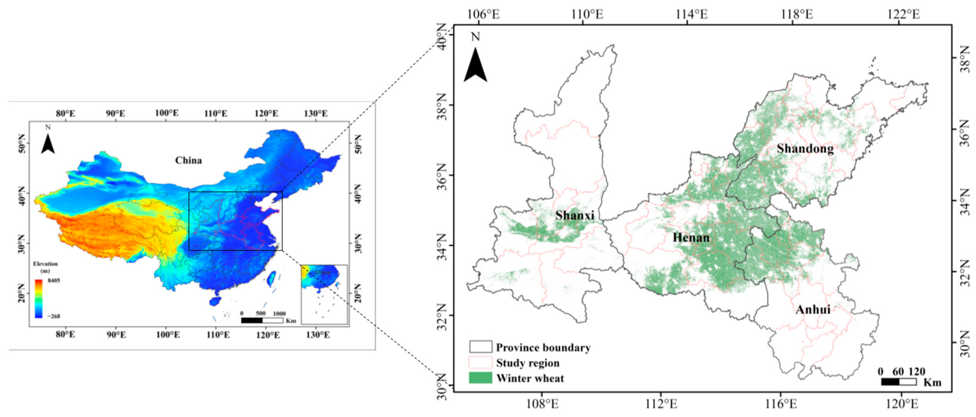
2.1. Study Area
2.2. Data
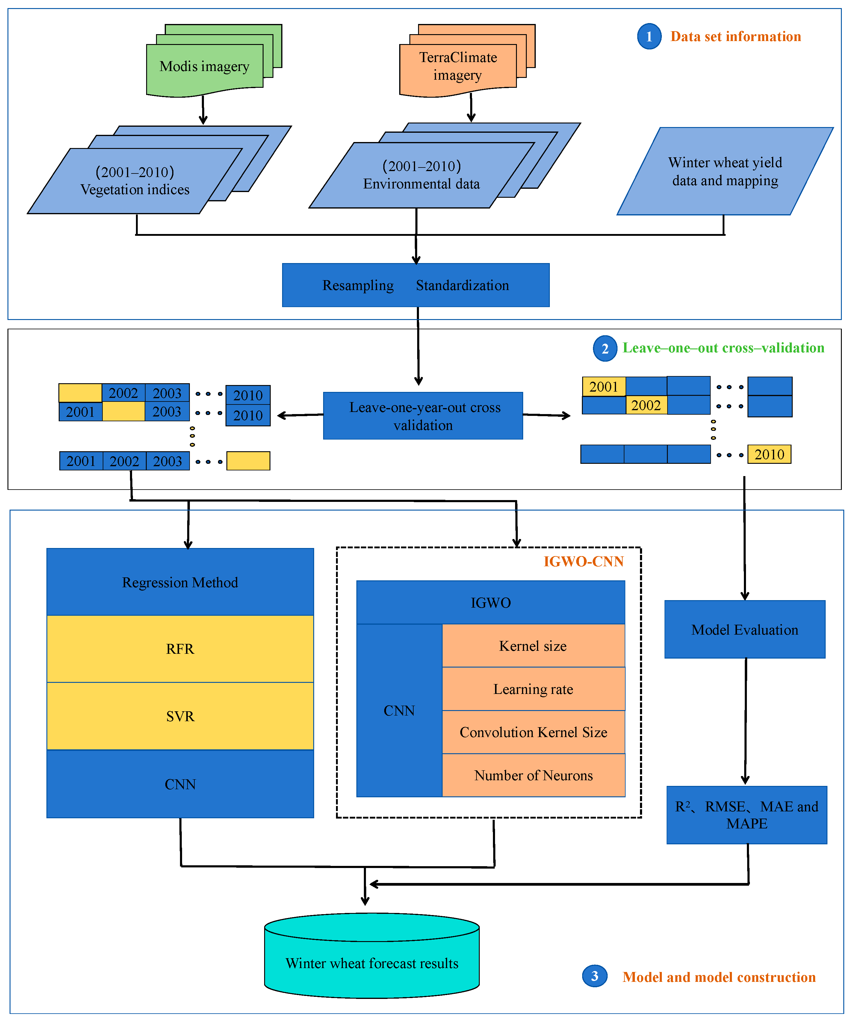
2.3. Methods
2.3.1. Models
2.3.2. Verification Method
2.3.3. Performance Evaluation
3. Results
3.1. Experimental Results and Analysis
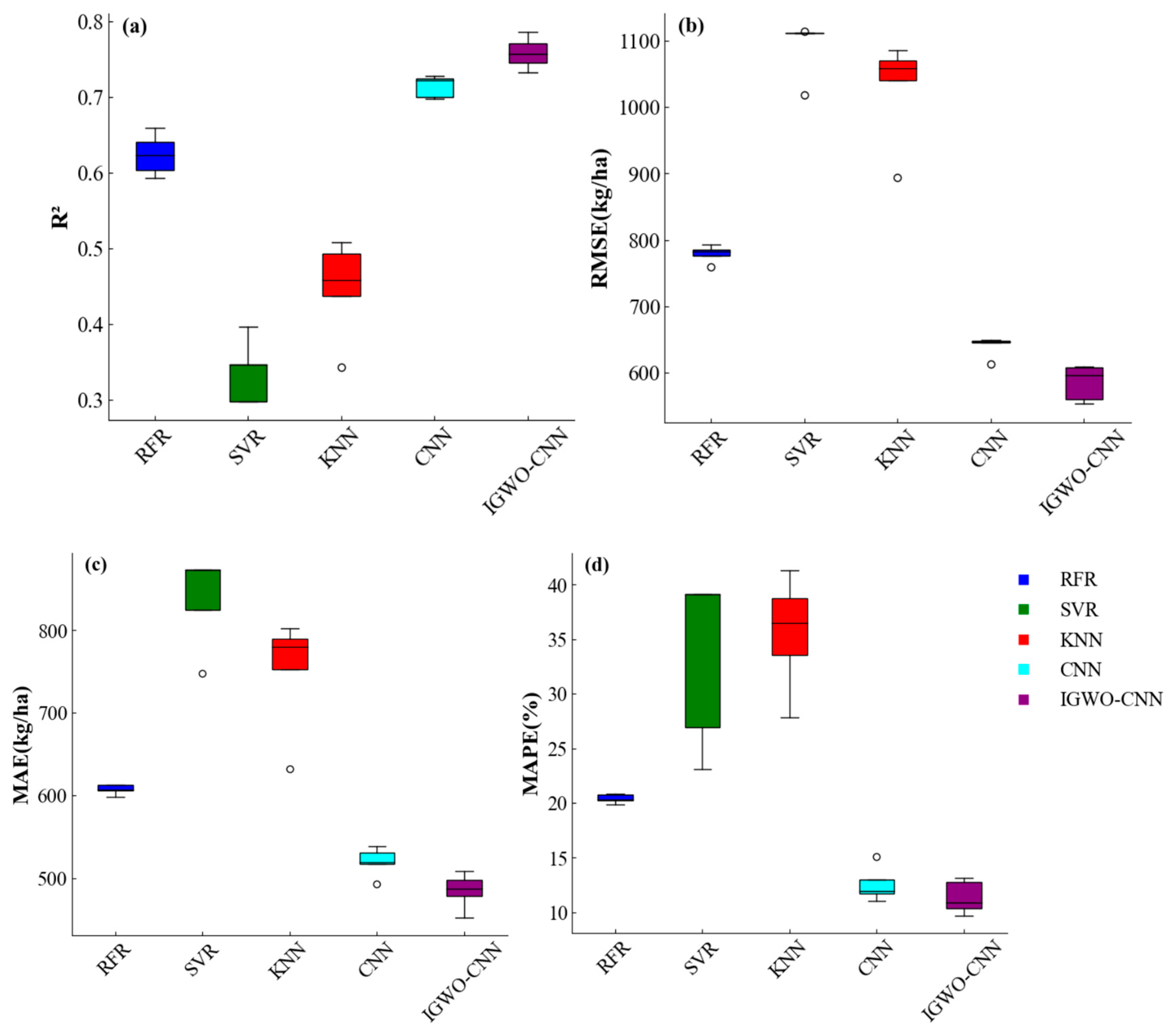
3.2. Prediction Results for Winter Wheat Yield Using Different Models
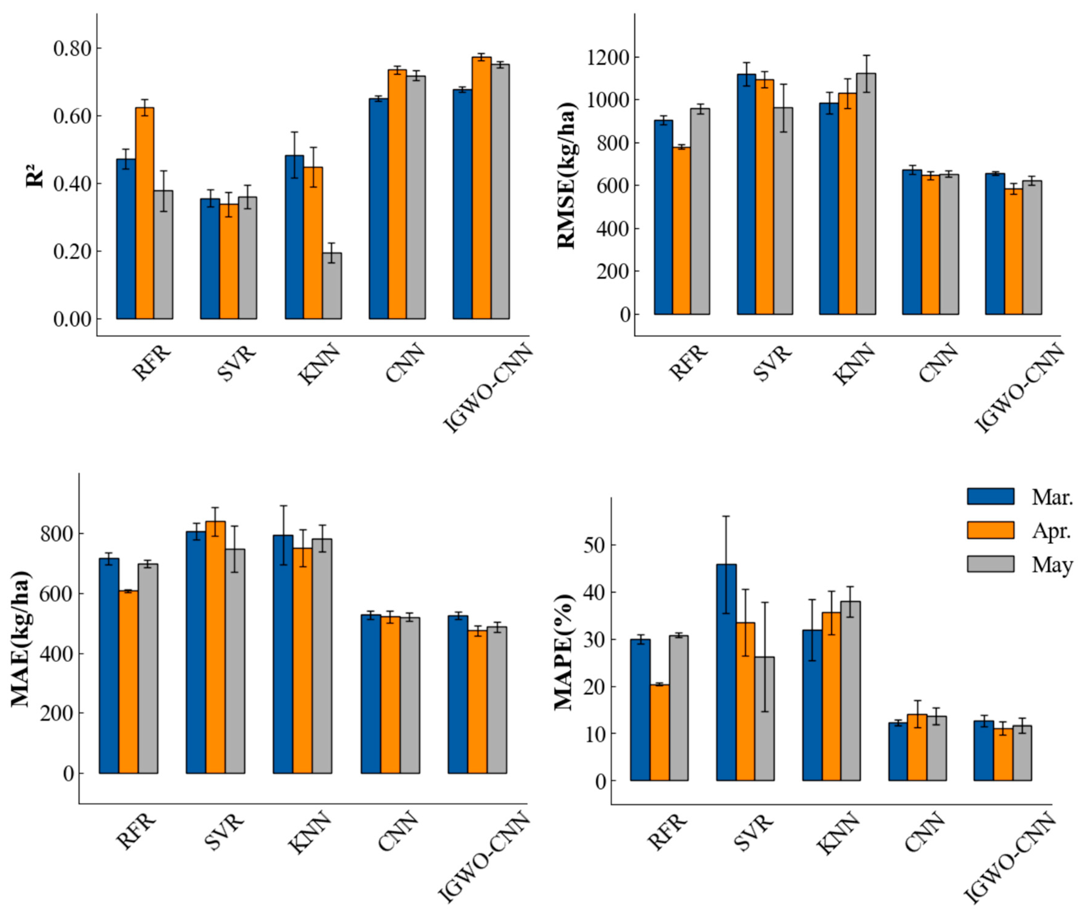
3.3. Comparison of Winter Wheat Yield Forecasts in Different Months
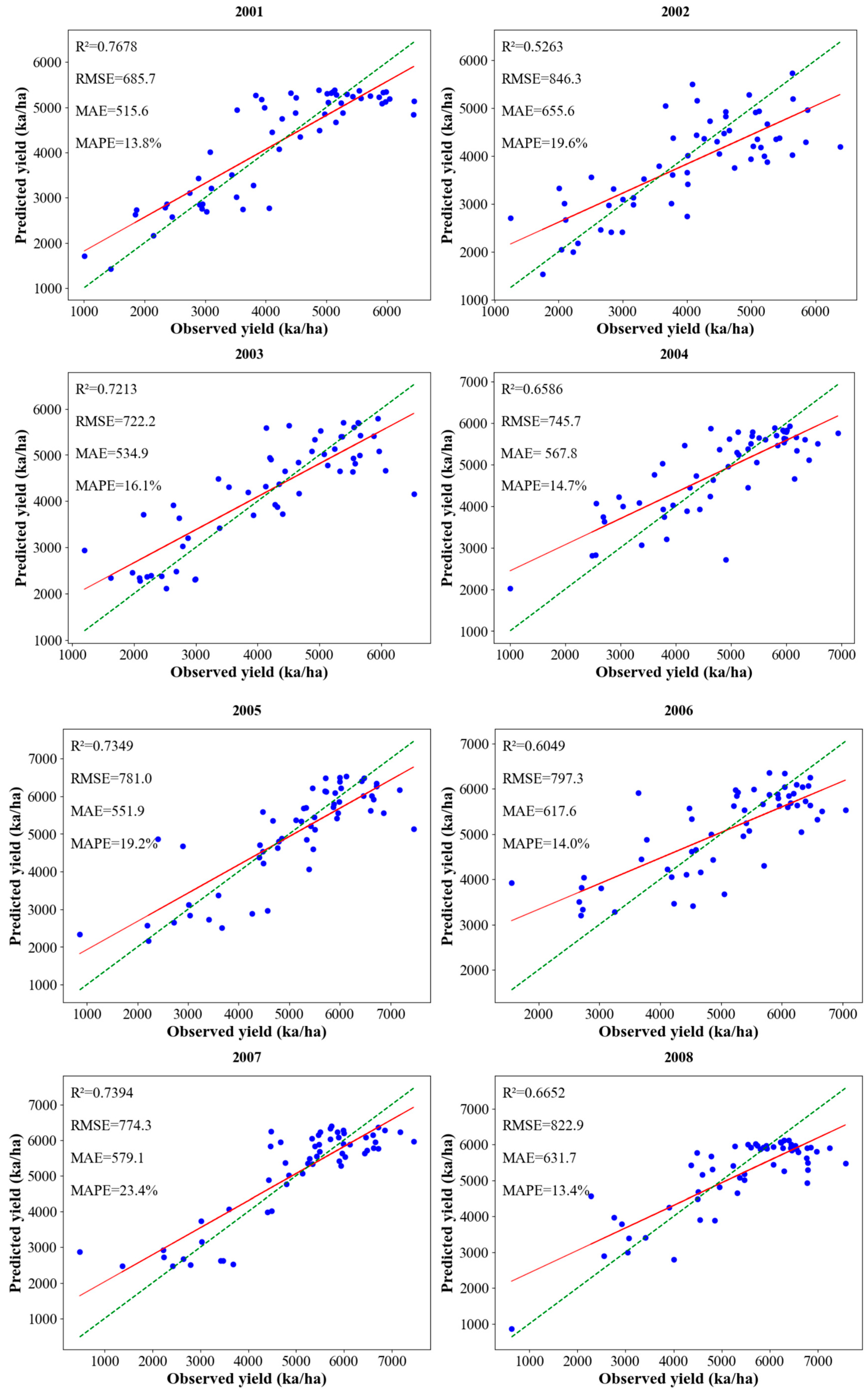
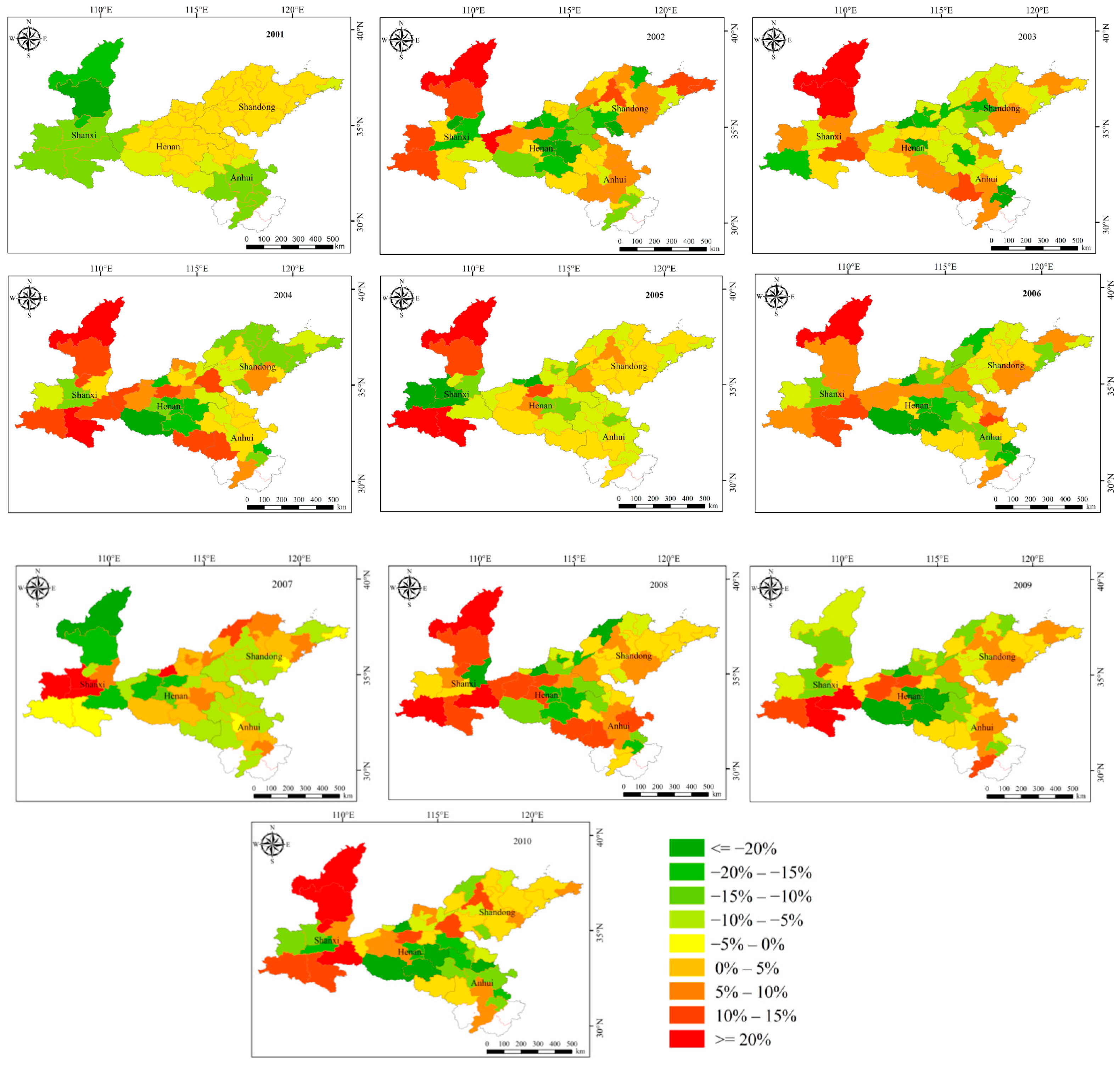
3.4. Comparison of Prediction Results in Different Years Based on IGWO-CNN Model
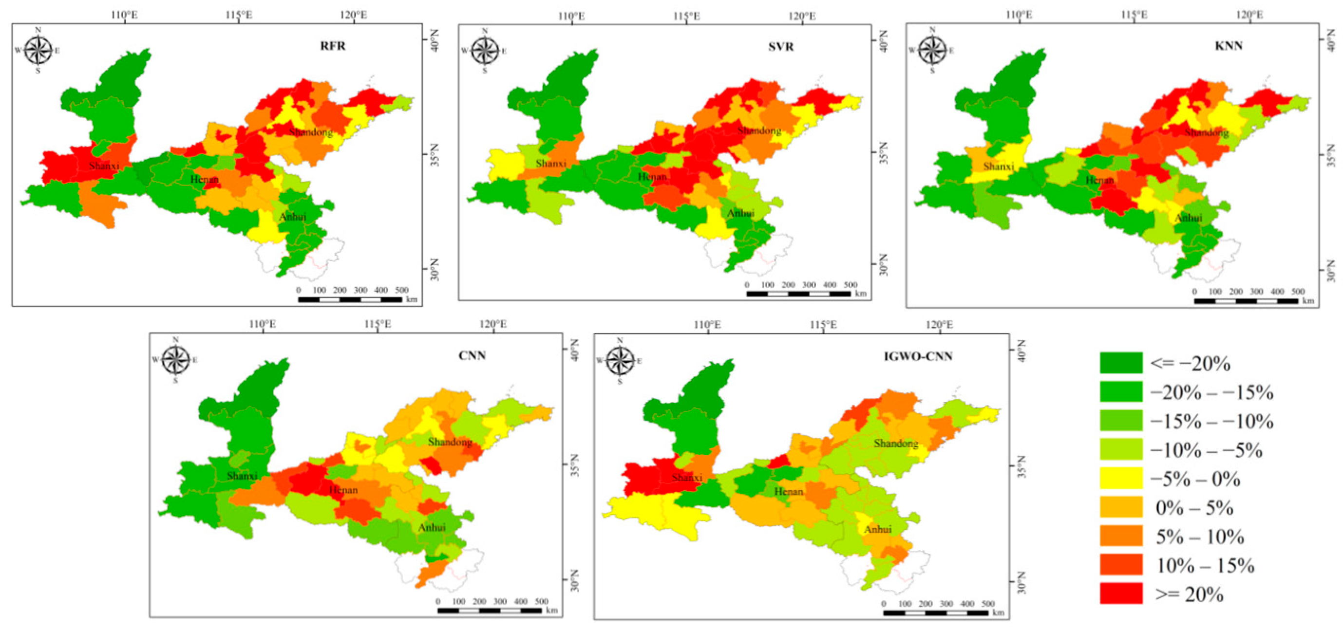
3.5. Spatial Distribution and Error Analysis of Winter Wheat Yield Forecast
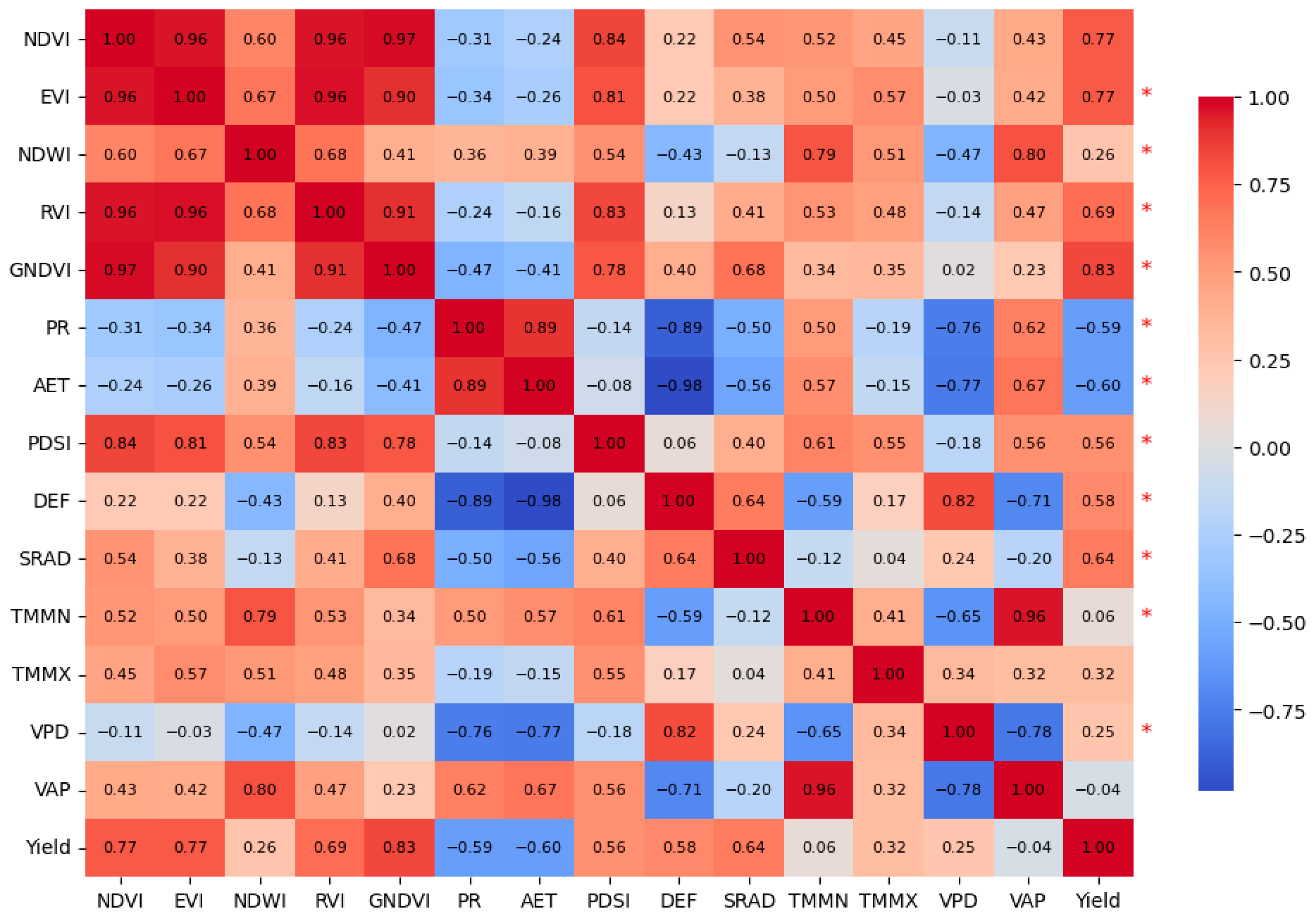
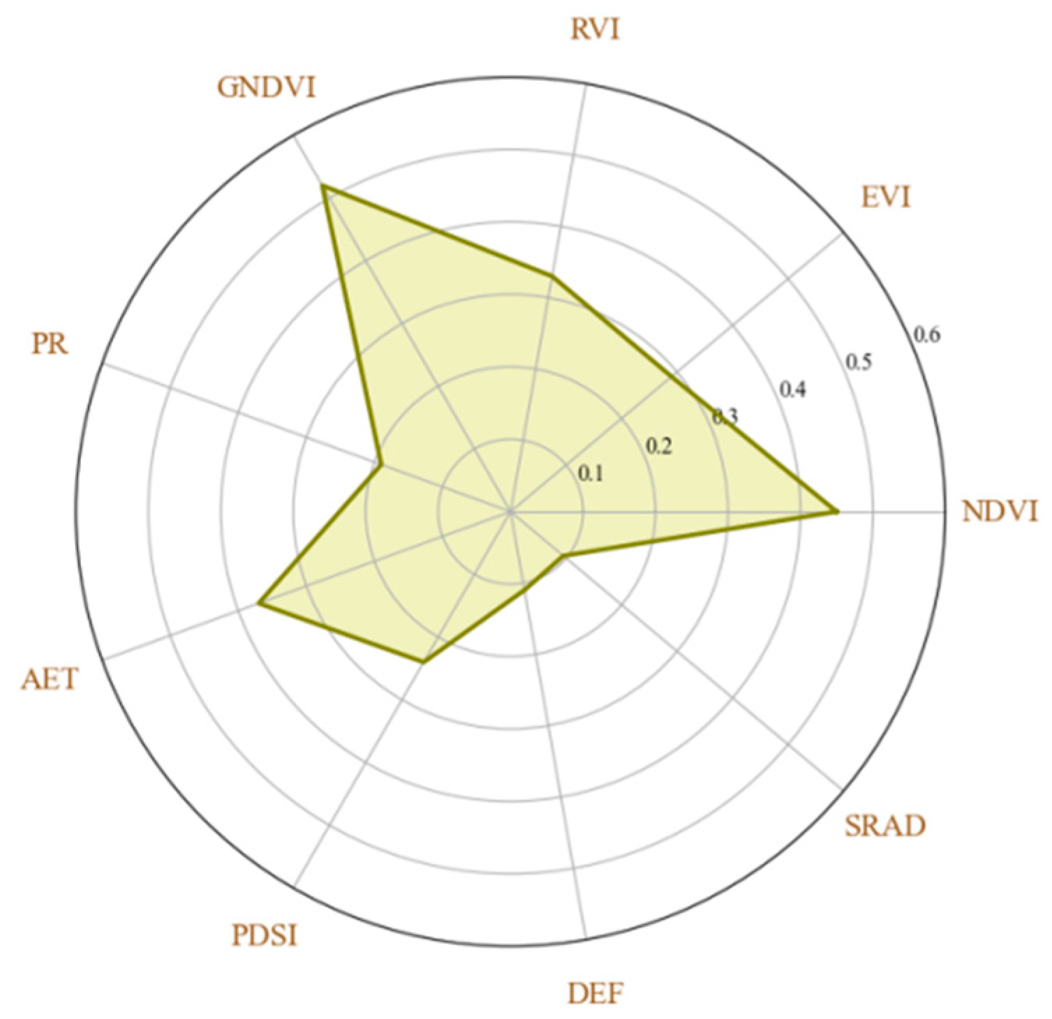
3.6. Importance of Individual Indicators in Yield Estimation
4. Discussion
5. Conclusions
Author Contributions
Funding
Data Availability Statement
Conflicts of Interest
References
- Gupta, R.; Meghwal, M.; Prabhakar, P.K. Bioactive compounds of pigmented wheat (Triticum aestivum): Potential benefits in human health. Trends Food Sci. Technol. 2021, 110, 240–252. [Google Scholar] [CrossRef]
- Omotoso, A.B.; Letsoalo, S.; Olagunju, K.O.; Tshwene, C.S.; Omotayo, A.O. Climate change and variability in sub-Saharan Africa: A systematic review of trends and impacts on agriculture. J. Clean. Prod. 2023, 414, 137487. [Google Scholar] [CrossRef]
- Nordmeyer, E.F.; Danne, M.; Musshoff, O. Can satellite-retrieved data increase farmers’ willingness to insure against drought?—Insights from Germany. Agric. Syst. 2023, 211, 103718. [Google Scholar] [CrossRef]
- Ali, A.; Hussain, T.; Tantashutikun, N.; Hussain, N.; Cocetta, G. Application of Smart Techniques, Internet of Things and Data Mining for Resource Use Efficient and Sustainable Crop Production. Agriculture 2023, 13, 397. [Google Scholar] [CrossRef]
- Casagli, N.; Intrieri, E.; Tofani, V.; Gigli, G.; Raspini, F. Landslide detection, monitoring and prediction with remote-sensing techniques. Nat. Rev. Earth Environ. 2023, 4, 51–64. [Google Scholar] [CrossRef]
- Sheikh, M.; Iqra, F.; Ambreen, H.; Pravin, K.A.; Ikra, M.; Chung, Y.S. Integrating artificial intelligence and high-throughput phenotyping for crop improvement. J. Integr. Agric. 2024, 23, 1787–1802. [Google Scholar] [CrossRef]
- Clark, R.; Dahlhaus, P.; Robinson, N.; Larkins, J.-a.; Morse-McNabb, E. Matching the model to the available data to predict wheat, barley, or canola yield: A review of recently published models and data. Agric. Syst. 2023, 211, 103749. [Google Scholar] [CrossRef]
- Kumar, R.; Agrawal, N. Analysis of multi-dimensional Industrial IoT (IIoT) data in Edge–Fog–Cloud based architectural frameworks: A survey on current state and research challenges. J. Ind. Inf. Integr. 2023, 35, 100504. [Google Scholar] [CrossRef]
- Hai, A.; Bharath, G.; Patah, M.F.A.; Daud, W.M.A.W.; Rambabu, K.; Show, P.; Banat, F. Machine learning models for the prediction of total yield and specific surface area of biochar derived from agricultural biomass by pyrolysis. Environ. Technol. Innov. 2023, 30, 103071. [Google Scholar] [CrossRef]
- Luo, L.; Sun, S.; Xue, J.; Gao, Z.; Zhao, J.; Yin, Y.; Gao, F.; Luan, X. Crop yield estimation based on assimilation of crop models and remote sensing data: A systematic evaluation. Agric. Syst. 2023, 210, 103711. [Google Scholar] [CrossRef]
- Ahmed, S.F.; Alam, M.S.B.; Hassan, M.; Rozbu, M.R.; Ishtiak, T.; Rafa, N.; Mofijur, M.; Shawkat Ali, A.B.M.; Gandomi, A.H. Deep learning modelling techniques: Current progress, applications, advantages, and challenges. Artif. Intell. Rev. 2023, 56, 13521–13617. [Google Scholar] [CrossRef]
- Naghdyzadegan Jahromi, M.; Zand-Parsa, S.; Razzaghi, F.; Jamshidi, S.; Didari, S.; Doosthosseini, A.; Pourghasemi, H.R. Developing machine learning models for wheat yield prediction using ground-based data, satellite-based actual evapotranspiration and vegetation indices. Eur. J. Agron. 2023, 146, 126820. [Google Scholar] [CrossRef]
- Arshad, S.; Kazmi, J.H.; Javed, M.G.; Mohammed, S. Applicability of machine learning techniques in predicting wheat yield based on remote sensing and climate data in Pakistan, South Asia. Eur. J. Agron. 2023, 147, 126837. [Google Scholar] [CrossRef]
- Dhaliwal, D.S.; Williams, M.M. Sweet corn yield prediction using machine learning models and field-level data. Precis. Agric. 2024, 25, 51–64. [Google Scholar] [CrossRef]
- Mütter, F.; Berger, C.; Königshofer, B.; Höber, M.; Hochenauer, C.; Subotić, V. Artificial intelligence for solid oxide fuel cells: Combining automated high accuracy artificial neural network model generation and genetic algorithm for time-efficient performance prediction and optimization. Energy Convers. Manag. 2023, 291, 117263. [Google Scholar] [CrossRef]
- Vigya; Shiva, C.K.; Vedik, B.; Raj, S.; Mahapatra, S.; Mukherjee, V. A novel chaotic chimp sine cosine algorithm part-II: Automatic generation control of complex power system. Chaos Solitons Fractals 2023, 173, 113673. [Google Scholar] [CrossRef]
- Bian, K.; Priyadarshi, R. Machine learning optimization techniques: A Survey, classification, challenges, and Future Research Issues. Arch. Comput. Methods Eng. 2024, 31, 4209–4233. [Google Scholar] [CrossRef]
- Han, W.; Gu, Q.; Gu, H.; Xia, R.; Gao, Y.; Zhou, Z.; Luo, K.; Fang, X.; Zhang, Y. Design of Chili Field Navigation System Based on Multi-Sensor and Optimized TEB Algorithm. Agronomy 2024, 14, 2872. [Google Scholar] [CrossRef]
- Tian, H.; Wang, P.; Tansey, K.; Zhang, S.; Zhang, J.; Li, H. An IPSO-BP neural network for estimating wheat yield using two remotely sensed variables in the Guanzhong Plain, PR China. Comput. Electron. Agric. 2020, 169, 105180. [Google Scholar] [CrossRef]
- Hatta, N.M.; Zain, A.M.; Sallehuddin, R.; Shayfull, Z.; Yusoff, Y. Recent studies on optimisation method of Grey Wolf Optimiser (GWO): A review (2014–2017). Artif. Intell. Rev. 2019, 52, 2651–2683. [Google Scholar] [CrossRef]
- Castillo-García, G.; Morán-Fernández, L.; Bolón-Canedo, V. Feature selection for domain adaptation using complexity measures and swarm intelligence. Neurocomputing 2023, 548, 126422. [Google Scholar] [CrossRef]
- Bardhan, A.; Biswas, R.; Kardani, N.; Iqbal, M.; Samui, P.; Singh, M.P.; Asteris, P.G. A novel integrated approach of augmented grey wolf optimizer and ANN for estimating axial load carrying-capacity of concrete-filled steel tube columns. Constr. Build. Mater. 2022, 337, 127454. [Google Scholar] [CrossRef]
- Md-Tahir, H.; Mahmood, H.S.; Husain, M.; Khalil, A.; Shoaib, M.; Ali, M.; Ali, M.M.; Tasawar, M.; Khan, Y.A.; Awan, U.K.; et al. Localized Crop Classification by NDVI Time Series Analysis of Remote Sensing Satellite Data; Applications for Mechanization Strategy and Integrated Resource Management. AgriEngineering 2024, 6, 2429–2444. [Google Scholar] [CrossRef]
- Dong, J.; Fu, Y.; Wang, J.; Tian, H.; Fu, S.; Niu, Z.; Han, W.; Zheng, Y.; Huang, J.; Yuan, W. Early-season mapping of winter wheat in China based on Landsat and Sentinel images. Earth Syst. Sci. Data 2020, 12, 3081–3095. [Google Scholar] [CrossRef]
- Cihlar, J.; St.-Laurent, L.; Dyer, J.A. Relation between the normalized difference vegetation index and ecological variables. Remote Sens. Environ. 1991, 35, 279–298. [Google Scholar] [CrossRef]
- Kyratzis, A.C.; Skarlatos, D.P.; Menexes, G.C.; Vamvakousis, V.F.; Katsiotis, A. Assessment of Vegetation Indices Derived by UAV Imagery for Durum Wheat Phenotyping under a Water Limited and Heat Stressed Mediterranean Environment. Front. Plant Sci. 2017, 8, 1114. [Google Scholar] [CrossRef]
- Gao, B.-c. NDWI—A normalized difference water index for remote sensing of vegetation liquid water from space. Remote Sens. Environ. 1996, 58, 257–266. [Google Scholar] [CrossRef]
- Huete, A.R. A soil-adjusted vegetation index (SAVI). Remote Sens. Environ. 1988, 25, 295–309. [Google Scholar] [CrossRef]
- Gregow, E.; Saltikoff, E.; Albers, S.; Hohti, H. Precipitation accumulation analysis–assimilation of radar-gauge measurements and validation of different methods. Hydrol. Earth Syst. Sci. 2013, 17, 4109–4120. [Google Scholar] [CrossRef]
- Hadadi, F.; Moazenzadeh, R.; Mohammadi, B. Estimation of actual evapotranspiration: A novel hybrid method based on remote sensing and artificial intelligence. J. Hydrol. 2022, 609, 127774. [Google Scholar] [CrossRef]
- Amirhajloo, S.; Gheysari, M.; Shayannejad, M.; Shirvani, M. Selection of the best nitrogen fertilizer management scenario in wheat based on Palmer drought severity index with an environmental perspective. Eur. J. Agron. 2023, 151, 126980. [Google Scholar] [CrossRef]
- Grossman, J.J. Phenological physiology: Seasonal patterns of plant stress tolerance in a changing climate. New Phytol. 2023, 237, 1508–1524. [Google Scholar] [CrossRef] [PubMed]
- Hao, H.; Yao, J.; Chen, Y.; Xu, J.; Li, Z.; Duan, W.; Ismail, S.; Wang, G. Ecological transitions in Xinjiang, China: Unraveling the impact of climate change on vegetation dynamics (1990–2020). J. Geogr. Sci. 2024, 34, 1039–1064. [Google Scholar] [CrossRef]
- Kakhani, N.; Rangzan, M.; Jamali, A.; Attarchi, S.; Alavipanah, S.K.; Mommert, M.; Tziolas, N.; Scholten, T. SSL-SoilNet: A Hybrid Transformer-Based Framework with Self-Supervised Learning for Large-Scale Soil Organic Carbon Prediction. IEEE Trans. Geosci. Remote Sens. 2024, 62, 4509915. [Google Scholar] [CrossRef]
- Yang, F.; Zhang, D.; Zhang, Y.; Zhang, Y.; Han, Y.; Zhang, Q.; Zhang, Q.; Zhang, C.; Liu, Z.; Wang, K. Prediction of corn variety yield with attribute-missing data via graph neural network. Comput. Electron. Agric. 2023, 211, 108046. [Google Scholar] [CrossRef]
- Noguera, I.; Vicente-Serrano, S.M.; Peña-Angulo, D.; Domínguez-Castro, F.; Juez, C.; Tomás-Burguera, M.; Lorenzo-Lacruz, J.; Azorin-Molina, C.; Halifa-Marín, A.; Fernández-Duque, B.; et al. Assessment of vapor pressure deficit variability and trends in Spain and possible connections with soil moisture. Atmos. Res. 2023, 285, 106666. [Google Scholar] [CrossRef]
- Guo, W.; Huang, S.; Huang, Q.; She, D.; Shi, H.; Leng, G.; Li, J.; Cheng, L.; Gao, Y.; Peng, J. Precipitation and vegetation transpiration variations dominate the dynamics of agricultural drought characteristics in China. Sci. Total Environ. 2023, 898, 165480. [Google Scholar] [CrossRef] [PubMed]
- Guo, J.; Zan, X.; Wang, L.; Lei, L.; Ou, C.; Bai, S. A random forest regression with Bayesian optimization-based method for fatigue strength prediction of ferrous alloys. Eng. Fract. Mech. 2023, 293, 109714. [Google Scholar] [CrossRef]
- Roy, A.; Chakraborty, S. Support vector machine in structural reliability analysis: A review. Reliab. Eng. Syst. Saf. 2023, 233, 109126. [Google Scholar] [CrossRef]
- Ngu, J.C.Y.; Yeo, W.S.; Thien, T.F.; Nandong, J. A comprehensive overview of the applications of kernel functions and data-driven models in regression and classification tasks in the context of software sensors. Appl. Soft Comput. 2024, 164, 111975. [Google Scholar] [CrossRef]
- Wang, A.X.; Chukova, S.S.; Nguyen, B.P. Ensemble k-nearest neighbors based on centroid displacement. Inf. Sci. 2023, 629, 313–323. [Google Scholar] [CrossRef]
- Agrawal, P.; Gnanaprakash, R.; Dhawane, S.H. Prediction of Biodiesel Yield Employing Machine Learning: Interpretability Analysis via Shapley Additive Explanations. Fuel 2024, 359, 130516. [Google Scholar] [CrossRef]
- Yang, Y.; Zhang, Y.; Cheng, Y.; Lei, Z.; Gao, X.; Huang, Y.; Ma, Y. Using one-dimensional convolutional neural networks and data augmentation to predict thermal production in geothermal fields. J. Clean. Prod. 2023, 387, 135879. [Google Scholar] [CrossRef]
- Guo, Z.; Yang, C.; Wang, D.; Liu, H. A novel deep learning model integrating CNN and GRU to predict particulate matter concentrations. Process Saf. Environ. Prot. 2023, 173, 604–613. [Google Scholar] [CrossRef]
- Singh, P.; Chaudhury, S.; Panigrahi, B.K. Hybrid MPSO-CNN: Multi-level Particle Swarm optimized hyperparameters of Convolutional Neural Network. Swarm Evol. Comput. 2021, 63, 100863. [Google Scholar] [CrossRef]
- Gad, A.G.; Houssein, E.H.; Zhou, M.; Suganthan, P.N.; Wazery, Y.M. Damping-Assisted Evolutionary Swarm Intelligence for Industrial IoT Task Scheduling in Cloud Computing. IEEE Internet Things J. 2024, 11, 1698–1710. [Google Scholar] [CrossRef]
- Yu, X.; Hu, Z. A multi-strategy driven reinforced hierarchical operator in the grey wolf optimizer for feature selection. Inf. Sci. 2024, 677, 120924. [Google Scholar] [CrossRef]
- Nguyen, T.; Kashani, A.; Ngo, T.; Bordas, S. Deep neural network with high-order neuron for the prediction of foamed concrete strength. Comput.-Aided Civ. Infrastruct. Eng. 2019, 34, 316–332. [Google Scholar] [CrossRef]
- Friedman, J. The Elements of Statistical Learning: Data Mining, Inference, and Prediction; Springer: Berlin/Heidelberg, Germany, 2009. [Google Scholar]
- Ghimire, S.; Deo, R.C.; Casillas-Pérez, D.; Salcedo-Sanz, S. Efficient daily electricity demand prediction with hybrid deep-learning multi-algorithm approach. Energy Convers. Manag. 2023, 297, 117707. [Google Scholar] [CrossRef]
- Huo, D.; Malik, A.W.; Ravana, S.D.; Rahman, A.U.; Ahmedy, I. Mapping smart farming: Addressing agricultural challenges in data-driven era. Renew. Sustain. Energy Rev. 2024, 189, 113858. [Google Scholar] [CrossRef]
- Jalali, S.M.J.; Ahmadian, S.; Khodayar, M.; Khosravi, A.; Shafie-khah, M.; Nahavandi, S.; Catalão, J.P.S. An advanced short-term wind power forecasting framework based on the optimized deep neural network models. Int. J. Electr. Power Energy Syst. 2022, 141, 108143. [Google Scholar] [CrossRef]
- Abou Houran, M.; Salman Bukhari, S.M.; Zafar, M.H.; Mansoor, M.; Chen, W. COA-CNN-LSTM: Coati optimization algorithm-based hybrid deep learning model for PV/wind power forecasting in smart grid applications. Appl. Energy 2023, 349, 121638. [Google Scholar] [CrossRef]
- Hashemi, M.G.Z.; Tan, P.-N.; Jalilvand, E.; Wilke, B.; Alemohammad, H.; Das, N.N. Yield estimation from SAR data using patch-based deep learning and machine learning techniques. Comput. Electron. Agric. 2024, 226, 109340. [Google Scholar] [CrossRef]
- Zheng, H.; Zheng, Z.; Hu, R.; Xiao, B.; Wu, Y.; Yu, F.; Liu, X.; Li, G.; Deng, L. Temporal dendritic heterogeneity incorporated with spiking neural networks for learning multi-timescale dynamics. Nat. Commun. 2024, 15, 277. [Google Scholar] [CrossRef] [PubMed]
- Phiphitphatphaisit, S.; Surinta, O. Multi-layer adaptive spatial-temporal feature fusion network for efficient food image recognition. Expert Syst. Appl. 2024, 255, 124834. [Google Scholar] [CrossRef]
- Jonathan, A.L.; Cai, D.; Ukwuoma, C.C.; Nkou, N.J.J.; Huang, Q.; Bamisile, O. A radiant shift: Attention-embedded CNNs for accurate solar irradiance forecasting and prediction from sky images. Renew. Energy 2024, 234, 121133. [Google Scholar] [CrossRef]
- Yuan, C.; Zhao, D.; Heidari, A.A.; Liu, L.; Chen, Y.; Chen, H. Polar lights optimizer: Algorithm and applications in image segmentation and feature selection. Neurocomputing 2024, 607, 128427. [Google Scholar] [CrossRef]
- Zhuang, H.; Zhang, Z.; Cheng, F.; Han, J.; Luo, Y.; Zhang, L.; Cao, J.; Zhang, J.; He, B.; Xu, J.; et al. Integrating data assimilation, crop model, and machine learning for winter wheat yield forecasting in the North China Plain. Agric. For. Meteorol. 2024, 347, 109909. [Google Scholar] [CrossRef]
- Fischer, T.; Gonzalez, F.G.; Miralles, D.J. Breeding for increased grains/m2 in wheat crops through targeting critical period duration: A review. Field Crops Res. 2024, 316, 109497. [Google Scholar] [CrossRef]
- Zhang, B.; Gu, L.; Dai, M.; Bao, X.; Sun, Q.; Zhang, M.; Qu, X.; Li, Z.; Zhen, W.; Gu, X. Estimation of grain filling rate of winter wheat using leaf chlorophyll and LAI extracted from UAV images. Field Crops Res. 2024, 306, 109198. [Google Scholar] [CrossRef]
- Lu, J.; Fu, H.; Tang, X.; Liu, Z.; Huang, J.; Zou, W.; Chen, H.; Sun, Y.; Ning, X.; Li, J. GOA-optimized deep learning for soybean yield estimation using multi-source remote sensing data. Sci. Rep. 2024, 14, 7097. [Google Scholar] [CrossRef] [PubMed]
- Li, J.; He, Z.; Zhou, G.; Yan, S.; Zhang, J. DeepAT: A Deep Learning Wheat Phenotype Prediction Model Based on Genotype Data. Agronomy 2024, 14, 2756. [Google Scholar] [CrossRef]
- Chen, L.; Zhong, X.; Li, H.; Wu, J.; Lu, B.; Chen, D.; Xie, S.-P.; Wu, L.; Chao, Q.; Lin, C.; et al. A machine learning model that outperforms conventional global subseasonal forecast models. Nat. Commun. 2024, 15, 6425. [Google Scholar] [CrossRef]
- Xue, S.; Fang, Z.; van Riper, C.; He, W.; Li, X.; Zhang, F.; Wang, T.; Cheng, C.; Zhou, Q.; Huang, Z.; et al. Ensuring China’s food security in a geographical shift of its grain production: Driving factors, threats, and solutions. Resour. Conserv. Recycl. 2024, 210, 107845. [Google Scholar] [CrossRef]


| Data | Variable | Temporal Resolution | Spatial Resolution | Source |
|---|---|---|---|---|
| Vegetation indices | NDVI, EVI, NDWI, RVI, GNDVI | 16-day | 500 m | MOD13A1 Version 6.1 product |
| Environmental data | PR, AET, PDSI, DEF, SRAD, TMMN, TMMX, VPD, VAP | Monthly | 1 km | TerraClimate datasets |
| Winter wheat yield and planting area | Planting area | Year | 30 m | https://doi.org/10.5194/essd-12-3081-2020 (accessed on 23 June 2024) |
| Yield data for winter wheat | Year | City | https://tjj.henan.gov.cn/ (accessed on 23 June 2024) | |
| Year | City | https://tjj.shaanxi.gov.cn/ (accessed on 26 June 2024) | ||
| Year | City | https://tjj.shandong.gov.cn/ (accessed on 26 June 2024) | ||
| Year | City | https://tjj.ah.gov.cn/ (accessed on 26 June 2024) |
| Model | Hyperparameter | Selected Value |
|---|---|---|
| RFR | n_estimators | 200 |
| min_samples_leaf | 2 | |
| random_state | 2 | |
| SVR | Kerne | RBF |
| gamma | 0.00001 | |
| Epsilon | 0.001 | |
| Regularization Parameter (C) | 1000 | |
| KNN | n_neighbors | 5 |
| weights | Uniform | |
| algorithm | Auto | |
| leaf_size | 30 | |
| p | 2 | |
| CNN | filters | 64, 128, 512 |
| kernel_size | 3 | |
| dense_layers | 2 | |
| dense_neurons | 32 | |
| learning_rate | 0.0006 | |
| loss_function | Mse | |
| batch_size | 256 | |
| epochs | 1000 | |
| IGWO-CNN | filters | 64, 128, 512 |
| kernel_size | 2 | |
| dense_layers | 2 | |
| dense_neurons | 70 | |
| learning_rate | 0.001 | |
| loss_function | Mse | |
| batch_size | 512 | |
| epochs | 1000 |
Disclaimer/Publisher’s Note: The statements, opinions and data contained in all publications are solely those of the individual author(s) and contributor(s) and not of MDPI and/or the editor(s). MDPI and/or the editor(s) disclaim responsibility for any injury to people or property resulting from any ideas, methods, instructions or products referred to in the content. |
© 2025 by the authors. Licensee MDPI, Basel, Switzerland. This article is an open access article distributed under the terms and conditions of the Creative Commons Attribution (CC BY) license (https://creativecommons.org/licenses/by/4.0/).
Share and Cite
Fu, H.; Lu, J.; Li, J.; Zou, W.; Tang, X.; Ning, X.; Sun, Y. Winter Wheat Yield Prediction Using Satellite Remote Sensing Data and Deep Learning Models. Agronomy 2025, 15, 205. https://doi.org/10.3390/agronomy15010205
Fu H, Lu J, Li J, Zou W, Tang X, Ning X, Sun Y. Winter Wheat Yield Prediction Using Satellite Remote Sensing Data and Deep Learning Models. Agronomy. 2025; 15(1):205. https://doi.org/10.3390/agronomy15010205
Chicago/Turabian StyleFu, Hongkun, Jian Lu, Jian Li, Wenlong Zou, Xuhui Tang, Xiangyu Ning, and Yue Sun. 2025. "Winter Wheat Yield Prediction Using Satellite Remote Sensing Data and Deep Learning Models" Agronomy 15, no. 1: 205. https://doi.org/10.3390/agronomy15010205
APA StyleFu, H., Lu, J., Li, J., Zou, W., Tang, X., Ning, X., & Sun, Y. (2025). Winter Wheat Yield Prediction Using Satellite Remote Sensing Data and Deep Learning Models. Agronomy, 15(1), 205. https://doi.org/10.3390/agronomy15010205