Improvement of Citrus Yield Prediction Using UAV Multispectral Images and the CPSO Algorithm

Abstract

Achieving timely and non-destructive assessments of crop yields is a key challenge in the agricultural field, as it is important for optimizing field management measures and improving crop productivity. To accurately and quickly predict citrus yield, this study obtained multispectral images of citrus fruit maturity through an unmanned aerial vehicle (UAV) and extracted multispectral vegetation indices (VIs) and texture features (T) from the images as feature variables. Extreme gradient boosting (XGB), random forest (RF), support vector machine (SVM), gaussian process regression (GPR), and multiple stepwise regression (MSR) models were used to construct citrus fruit number and quality prediction models. The results show that, for fruit number prediction, the XGB model performed best under the combined input of VIs and T, with an R² = 0.792 and an RMSE = 462 fruits. However, for fruit quality prediction, the RF model performed best when only the VIs were used, with an R² = 0.787 and an RMSE = 20.0 kg. Although the model accuracy was acceptable, the number of input feature variables used was large. To further improve the model prediction performance, we explored a method that utilizes a hybrid coding particle swarm optimization algorithm (CPSO) coupled with XGB and SVM models. The coupled models had a significant improvement in predicting the number and quality of citrus fruits, especially the model of CPSO coupled with XGB (CPSO-XGB). The CPSO-XGB model had fewer input features and higher accuracy, with an R² > 0.85. Finally, the Shapley additive explanations (SHAP) method was used to reveal the importance of the normalized difference chlorophyll index (NDCI) and the red band mean feature (MEA_R) when constructing the prediction model. The results of this study provide an application reference and a theoretical basis for the research on UAV remote sensing in relation to citrus yield.

1. Introduction

Citrus is one of the most important fruit crops in the world. It is widely cultivated worldwide, spanning from tropical to subtropical regions, mainly distributed in Asia, America, and Africa. Among them, Asia accounts for most of the global citrus yield, especially China, India, and Japan [1]. Citrus is rich in bioactive compounds that can reduce inflammation in the body and lower the risk of diseases associated with metabolic syndrome. Its fruits have a high nutritional value that is beneficial to human health, making it an important economic crop [2]. China has a long history of citrus cultivation, which is widely distributed. Its main production areas are located in the south of the Yangtze River, including the Sichuan, Jiangxi, and Guangxi provinces. The Jiangxi province has abundant resources of citrus products and Nanfeng tangerine is famous for its thin skin, less core, more juice, less residue, and sweet and sour taste [3]. National food security and personal living standards closely correlate with crop yield. Accurate predictions of crop yields before harvest plays an important role in formulating food policies, regulating food prices, and precision agriculture management [4]. Since most of our citrus industry is concentrated in hilly and mountainous environments, traditional manual yield measurements are time-consuming, laborious, and destructive. Therefore, it is necessary to estimate the yield of Nanfeng tangerine accurately, quickly, and non-destructively, an approach which can promote the development of the local citrus industry and improve the economic income of local fruit farmers.

In recent years, UAV remote sensing technology has been widely used in precision agriculture because of its convenient operation, flexibility, low cost, and high spatial and temporal resolution [5]. Many scholars have carried out research on fruit trees based on UAV remote sensing technology. Zhao et al. [6] obtained UAV multispectral images of apple orchards and used three machine learning models to estimate the nitrogen content of apple canopy leaves. They found that the random forest model had the highest accuracy. Zhang et al. [7] combined UAV images and texture information to estimate the leaf area index of kiwifruit trees by stepwise regression and random forest regression models. They found that texture information could improve the accuracy of model estimation. At present, there has been some progress in UAV remote sensing research on crop yield prediction. Maimaitijiang et al. [8] estimated soybean grain yield within the framework of deep neural networks based on visible light, multispectral, and thermal sensors carried by a UAV. They found that multimodal data fusion can provide relatively accurate and robust crop yield estimation. Sanches et al. [9] assessed the potential for yield prediction in sugarcane fields using visible light images obtained by a UAV and the leaf area index measured by the sensor. They found that the integration of the two was able to increase yield estimates by 10%. The above research displays that using UAV remote sensing technology to predict crop yield has excellent applicability and accuracy.

Since spectral reflectance alone may not be sufficient to estimate crop yield, many vegetation indices (VIs) calculated from spectral reflectance have been developed to estimate crop yield. Taşan et al. [10] used ten VIs and five machine learning models to estimate eggplant yield and found that the green index (GI) and the green vegetation index (GVI) had the greatest impact on eggplant yield. Lukas et al. [11] used UAV to obtain three VIs at the flowering stage of oilseed rape and found that high-precision yield prediction was achieved using the blue normalized difference vegetation index (BNDVI) and the normalized difference yellowness index (NDYI). In addition, although fewer studies are using remote sensing data to estimate fruit tree yield, Van Beek et al. [12] studied the time dependence of fruit yield estimated by VIs in irrigated and rainfed pear orchards and demonstrated a significant correlation between VIs and the fruit yield of pear trees. However, yield is a complex phenotypic trait that is influenced by many factors, including the external environment, gene type, and agronomic management [13]. These factors and their interactions have significant effects on crop yield; therefore, the estimation of crop yield is extremely complicated [14]. Previous studies have shown that a single VI may not provide a reliable estimate, and its performance depends on many factors, such as soil, climate, crop type, etc. To overcome the above problems, the morphological, geometric, and textural characteristics of the canopy have been combined with VIs for yield estimation, as it can give a better estimate. Chen et al. [15] extracted the morphological characteristics and VIs of individual apple trees from UAV lidar and multispectral images and developed an integrated model to predict the yield. This proved the effectiveness of the integrated model in predicting the yield of individual apple trees in orchards. Rahman et al. [16] used an artificial neural network model to integrate geometric (canopy area) and optical (VIs) data, evaluating the potential of high-resolution WorldView-3 (WV3) satellite images for estimating mango yield. This revealed that the model was able to predict the regional mango yield. Kang et al. [17] obtained multispectral images of winter wheat for three periods using a UAV and used VIs and texture features to establish yield estimation models. The results demonstrated that the model accuracy with texture features was higher than the accuracy achieved by single variable estimation.

With the rapid development of computer modeling technologies, machine learning (ML) technology has become an important link between UAV image information and crop yield. However, there are still two challenges in the ML simulation of crop yield. One is the problem of feature selection. There is usually strong collinearity between VIs obtained based on multispectral technology. That is, different VIs show similar effects in predicting yield, so it is difficult to obtain a robust VI-based crop yield prediction model. The tree-based model can evaluate features by calculating the contribution of different features and deleting redundant features by pruning operations to avoid overfitting the model. Zhang et al. [18] identified key features based on the feature selection method of the tree model, which enhanced the stability and predictive ability of the model for leaf area index estimation. Second, the accuracy and efficiency of the ML model depend largely on its internal model parameters. Compared with the common ML parameter calibration methods, the meta-heuristic algorithm has high precision and efficiency, which can provide the global optimal solution. Combining the meta-heuristic algorithm with the ML model can quickly find a more suitable parameter combination and improve the accuracy of the model. Wei et al. [19] used particle swarm optimization (PSO) to optimize the parameters of the least squares vector machine model for improving the inversion performance of suspended solid concentrations in waters.

Most of the previous studies have used UAV remote sensing technology to predict the yield of crops such as wheat [20], corn [21], and rice [22], while there are few studies on the yield prediction of citrus fruit trees. As an important feature, texture is often used for the interest recognition of objects or regions in images and image classification [23]. However, few scholars have used this method to estimate the yield of crops, especially citrus fruit trees. In addition, there are few reports on meta-heuristic optimization algorithms that can simultaneously achieve parameter optimization and feature selection. Therefore, this study took Nanfeng tangerine as the research object, collected UAV images of fruit maturity, calculated multispectral vegetation indices, and extracted multispectral image texture features. The two were used as feature variables, and five machine learning models, including extreme gradient boosting, random forest, support vector machine, Gaussian process regression, and multiple stepwise regression, were used to construct the prediction model of citrus fruit number and quality. The optimal model was selected by comparison and analysis, and the CPSO method was introduced to optimize the XGB and SVM models. The parameters and input features of the model were optimized at the same time, and the advantages of the CPSO method were proved compared with the selected optimal model. The aim of this study is to explore a method for predicting citrus yield by using UAV images, providing a theoretical reference for obtaining citrus yield quickly and accurately.

2. Materials and Methods

2.1. Study Area

This study was conducted at the rural water conservancy research and demonstration base (27°5′49″ N, 116°27′29″ E) in Nanfeng County, Fuzhou City, Jiangxi Province, China (Figure 1). This area belongs to the mid-subtropical monsoon climate zone. It is located in the hilly area of southeastern Jiangxi province. It is mild and humid, with sufficient rainfall and four distinct seasons. The average annual temperature is 19.8 °C, and the average annual rainfall is 1791.8 mm. The soil type is red soil, rich in iron and aluminum oxides, and belongs to the acidic soil and is suitable for planting citrus trees. The tested citrus variety was the Nanfeng tangerine. Nanfeng tangerine has a high reputation in the citrus market in China because of its thin skin, less core, more juice, and less residue.

2.2. Data Collection

2.2.1. Yield Data Acquisition

To ensure the growth difference of selected fruit trees, 118 sample trees were randomly selected in the experimental area during the citrus fruit maturity, and the labels with numbers were hung. In this experiment, yield data from citrus fruit trees were collected on 19 and 20 November 2023. For yield measurements, each sample tree circled was first manually counted and then weighed on an electronic platform scale. The number of fruits in the basket of each fruit tree was counted by the manual counting method. When weighing, the electronic platform scale was first placed on the horizontal ground and peeled, then the quality of the basket was measured. After counting, the basket was placed onto an electronic platform scale to be weighed and recorded. Finally, the quality of the basket needed to be subtracted to obtain the net quality of the fruits.

Table 1. Descriptive statistics of fruit number and quality in individual citrus plants.

	Max	Min	Median	Mean	Standard Deviation	Coefficient of Variation	Kurtosis	Skewness
Number/fruits	3890	0	960	1041	1005	0.965	−0.563	0.630
Quality/kg	151.0	0.0	44.5	45.4	42.2	0.931	−0.902	0.472

shows the statistical characteristics of fruit number and quality of the sample trees.

2.2.2. Multispectral Image Acquisition and Processing

On the day before the sample trees were picked (18 November 2023), the period of sunny weather, no wind, and fewer clouds was selected for the UAV multispectral image shooting to ensure image quality. The Dajiang Innovation (DJI) Mavic3 Multispectral (M3M) version UAV was used to obtain multispectral image data of citrus fruit tree canopy. The device was equipped with a four-band multispectral camera, i.e., green band, red band, red edge band, and near-infrared band. Its main parameters are shown in

Table 2. Main parameters of multispectral UAV.

UAV	Description	Sensor	Description
Name	DJI M3M	Bands	Green (560 nm ± 16 nm)
Flight altitude	50 m		Red (650 nm ± 16 nm)
Flight speed	4.4 m/s		Red Edge (730 nm ± 16 nm)
Satellite systems	GPS + Galileo + BeiDou		NIR (860 nm ± 26 nm)
Forward overlap	80%	Pixel	5 million
Side overlap	80%	Image dimension	2592 × 1944
Field of view	90°	Resolution	2.31 cm/pixel
Shooting interval	2 s	Image format	TIFF

. In addition, the DJI M3M UAV had an integrated light intensity sensor on the top and was equipped with the RTK module, which can compensate for the illumination of the image data and achieve centimeter-level high-precision positioning. Before collecting the UAV images, we set the flight route through the DJI pilot application on the remote controller and selected the equal-time photography mode and the ground-like flight mode.

After obtaining the image data, the UAV images needed to be preprocessed for image stitching, radiometric calibration, and image cropping. The multispectral images obtained from the UAV were recorded as a set of digital values, which needed to be converted into reflectivity by radiometric calibration [24]. Therefore, a manual takeoff of the UAV to photograph the radiometric calibration board was required before the flight. The multispectral images and the radiometric calibration board image were imported into the Pix4Dmapper software. First, the reflectance coefficients of the four multispectral bands of the radiometric calibration board were input in the processing options, then the images were stitched. After the stitching was completed, four single-band orthographic reflectance images were obtained. Finally, the ENVI5.3 software was used to cut the image to obtain the image data of the test area, followed by image synthesis and the extraction of the reflectance data from each band in the region of interest.

2.3. Selections of Vegetable Indices and Texture Features

Vegetation indices can simply and effectively estimate crop yield. Based on the results of previous studies, this study selected 16 multispectral band vegetation indices for machine learning modeling. The R language 4.3.0 platform was used to input the reflectance of each band in the region of interest in the orthophoto to calculate the vegetation indices. The texture information was calculated by using the gray level co-occurrence matrix (GLCM) of ENVI5.3. This method is based on second-order probability statistical filtering and analyzes the frequency distribution between pixels in a 3 × 3 local window. Each band was processed by eight statistical methods, with a total of 32 texture features. The specific calculation formulas for vegetation indices and texture features are shown in the following

Table 3. Vegetation indices used in this study.

No.	Vegetable Index	Equations	Reference
1	Green chlorophyll index	CIg = NIR/G − 1	[25]
2	Red edge chlorophyll index	CIre = NIR/RE − 1	[25]
3	Difference vegetation index	DVI = NIR − R	[26]
4	Green difference vegetation index	GDVI = NIR − G	[26]
5	Modified nonlinear index (MNLI)	MNLI = 1.5 × (NIR2 − R)/(NIR2 + R + 0.5)	[27]
6	Modified simple ratio (MSR)	MSR = (NIR/R − 1)/sqrt (NIR/R + 1)	[28]
7	Normalized difference red edge	NDRE = (NIR − RE)/(NIR + RE)	[29]
8	Normalized difference chlorophyll index	NDCI = (RE − R)/(RE + R)	[30]
9	Normalized difference vegetation index	NDVI = (NIR − R)/(NIR + R)	[31]
10	Renormalized difference vegetation index	RDVI = (NIR − R)/sqrt (NIR + R)	[32]
11	Red edge difference vegetation index	REDVI = NIR − RE	[33]
12	Ratio vegetation index	RVI = NIR/R	[34]
13	Soil-adjusted vegetation index	SAVI = 1.5 × (NIR − R)/(NIR + R + 0.5)	[35]
14	Optimized soil-adjusted vegetation index	OSAVI = (NIR − R)/(NIR + R + 0.16)	[36]
15	Spectrum vegetation index	SVI = (NIR − R)/(NIR + R)/NIR	[37]
16	Wide dynamic range vegetation index	WDRVI = (0.12 × NIR − R)/(0.12 × NIR + R)	[38]

Note 1: G, R, RE, and NIR indicate green, red, red edge, and near-infrared band reflectance, respectively.

and

Table 4. Texture features used in this study.

No.	Texture Feature	Equations	Reference
1	Mean	$ME{A}_i={\displaystyle \sum _{i,j=0}^{n-1}i}(P_{i,j}),$	[39]
		$ME{A}_j={\displaystyle \sum _{i,j=0}^{n-1}j}(P{i}_{i,j})$
2	Variance	$VA{R}_i={\displaystyle \sum _{i,j=0}^{n-1}{P}_{i,j}}{(i-ME{A}_i)}^2,$
		$VA{R}_j={\displaystyle \sum _{i,j=0}^{n-1}{P}_{i,j}}{(j-ME{A}_j)}^2$
3	Homogeneity	$HOM={\displaystyle \sum _{i,j=0}^{n-1}\frac{P_{i,j}}{1+{(i-j)}^2}}$
4	Contrast	$CON={\displaystyle \sum _{i,j=0}^{n-1}{P}_{i,j}}{(i-j)}^2$
5	Dissimilarity	$DIS={\displaystyle \sum _{i,j=0}^{n-1}{P}_{i,j}}|i-j|$
6	Entropy	$ENT={\displaystyle \sum _{i,j=0}^{n-1}P}(i,j)\log P(i,j)$
7	Second moment	$SEM={\displaystyle \sum _{i,j=0}^{n-1}{P}_{i,j}^2}$
8	Correlation	$COR={\displaystyle \sum _{i,j=0}^{n-1}{P}_{i,j}}{\displaystyle \frac{(i-ME{A}_i)(j-ME{A}_j)}{\sqrt{VA{R}_i^{2}VA{R}_j^2}}}$

Note 2: P, i, j, and n indicate the probability of simultaneous occurrence of j in GLCM, the grayscale value i, the grayscale value j, and the number of gray levels in an image, respectively.

.

2.4. Models and Analysis Methods

2.4.1. Machine Learning Models

The modeling methods included extreme gradient boosting (XGB), random forest (RF), support vector machine (SVM), Gaussian process regression (GPR), and multiple stepwise regression (MSR) models. Based on the R language 4.3.0 platform, this paper used the sample function to divide the dataset into a 70% modeling set and a 30% verification set to estimate the number and quality of citrus fruits. Among them, XGB is a machine learning algorithm based on the gradient boosting decision tree (GBDT) framework. It improves the prediction accuracy by constructing and combining multiple decision trees. Each tree is optimized based on the previous tree to minimize the loss function [40]. RF is an integrated learning algorithm based on multiple decision trees and the bagging technique, which improves the accuracy and stability of the model by constructing multiple decision trees and voting or averaging their predictions [41]. SVM is a supervised learning algorithm that can be used for classification and regression problems. It separates different types of data by finding the optimal hyperplane and introduces kernel functions so that SVM can effectively deal with nonlinear problems [42]. GPR is a Bayesian nonparametric regression model based on the Gaussian process which does not require a predefined model form and can adapt to complex data structures [43]. MSR is a multiple regression analysis model established by a stepwise search strategy, which can identify effective explanatory variables and simplify the model [44]. This study used the important function of the XGB algorithm to calculate the gain value of each feature which represents the contribution of the feature to the objective function when the node is split. The greater the gain value, the higher the importance of the feature. We screened 16 vegetation indices and 32 texture features, and defined a gain value greater than 0.05 as a high weight. On this basis, the image features that contributed greatly to the number and quality of citrus fruits were selected for the study in Section 3.2.

2.4.2. Compound Coded Particle Swarm Optimization (CPSO)

Particle swarm optimization (PSO) is an optimization algorithm based on swarm intelligence. It was proposed by Eberhart and Kennedy in 1995 [45] and was inspired by the foraging behavior of birds and sought the optimal solution by simulating the social behavior of biological groups such as birds or fish. In PSO, each solution is regarded as a particle in the search space, and each particle represents the potential solution to the problem. The particles fly in the search space updating their position and velocity by tracking two extrema: the individual extremum (pBest) and the global extremum (gBest). The position and velocity update formulas of particles in the algorithm are:

$$x_i(t+1)=x_i(t)+v_i(t+1)$$

(1)

$$v_i(t+1)=w\cdot v_i(t)+c_1\cdot r_1\cdot (pBes{t}_i-x_i(t))+c_2\cdot r_2\cdot (gBest-x_i(t))$$

(2)

where x_i is the position of the i-th particle, v_i is the corresponding speed, w is the inertia weight, r₁ and r₂ are random numbers in the range of [0, 1], and c₁ and c₂ are acceleration coefficients which mainly control the trend of particles moving to pBest and gBest. The binary particle swarm optimization (BPSO) is a discrete version of the particle swarm optimization algorithm which is used to solve discrete optimization problems [46]. In BPSO, the position of the particles is represented by a binary code, and the value of each dimension is 0 or 1. The velocity of the particle is no longer a continuous value but represents the probability of position change. The same as the PSO algorithm, both of them find the optimal solution by iteratively updating the position and velocity of the particles.

The hybrid coding particle swarm optimization algorithm uses a hybrid decimal and binary coding method combined with the traditional PSO algorithm and the binary PSO algorithm to optimize the machine learning model. The traditional PSO algorithm mainly optimizes the parameters of the model, while the binary PSO algorithm primarily filters the input parameters of the model. That is, when the result value is shown as 1, the feature is adopted as the input of the model; when the result value is shown as 0, the opposite is true. In this study, the CPSO algorithm was used to optimize the XGB and SVM models, as it can not only screen out the key input features, but also optimize the parameters of the model. Among them, the optimized parameters of the XGB model were the number of trees, the maximum tree depth, the learning rate, and the weight of child nodes. The parameters of the optimized SVM model were the regularization coefficient and the parameters of the Gaussian kernel function.

2.4.3. Shapley Additive Explanations (SHAP)

SHAP is a post-interpretability method for machine learning. It can assign a specific predictive importance value to each feature variable of the model and explain the prediction results of the model through the importance value [47]. In game theory, the SHAP value is originally used to evaluate the contribution of each participant to the common benefits in a cooperative game. In the field of machine learning, SHAP values are used to quantify the contribution of each feature to the model prediction. The calculation formula for the SHAP value is:

$$g(z^{\prime })={\varphi }_0+{\displaystyle \sum _{i=1}^M{\varphi }_i}{z}_i^{\prime }(z^{\prime }\in {\left\{0,1\right\}}^M)$$

(3)

where g is the explanatory model, M is the number of input features in the model, Φ₀ is the predicted mean of all training sets, and Φ_i is the marginal contribution of the variable i, namely the SHAP value. In this paper, the shapviz package of the R language is used to quantify the importance of each feature variable in the process of model modeling (Figure 2).

2.5. Statistical Indicators

We used the coefficient of determination (R²), the root mean square error (RMSE), the mean absolute error (MAE), and the normalized root mean square error (NRMSE) to evaluate the performance of the model. The calculation formulas for these statistical indicators are as follows:

$$R^2={\displaystyle \frac{{\left[{\displaystyle \sum _{i=1}^n(X_i-\overline{X})}(Y_i-\overline{Y})\right]}^2}{{\displaystyle \sum _{i=1}^n{(X_i-\overline{X})}^2}{\displaystyle \sum _{i=1}^n{(Y_i-\overline{Y})}^2}}}$$

(4)

$$RMSE=\sqrt{{\displaystyle \frac{1}{n}}{\displaystyle \sum _{i=1}^n{(Y_i-X_i)}^2}}$$

(5)

$$MAE={\displaystyle \frac{1}{n}}{\displaystyle \sum _{i=1}^n|}{Y}_i-X_i|$$

(6)

$$NRMSE={\displaystyle \frac{RMSE}{\overline{X}}}$$

(7)

where Y_i is the citrus yield value predicted by the model, X_i is the measured citrus yield value, $\overline{Y}$ is the average value of Y_i, $\overline{X}$ is the average value of X_i, and n is the data sample size. When RMSE, NRMSE, and MAE are close to 0 and R² is close to 1, the regression curve between the predicted value of the model and the measured value fits better.

3. Results

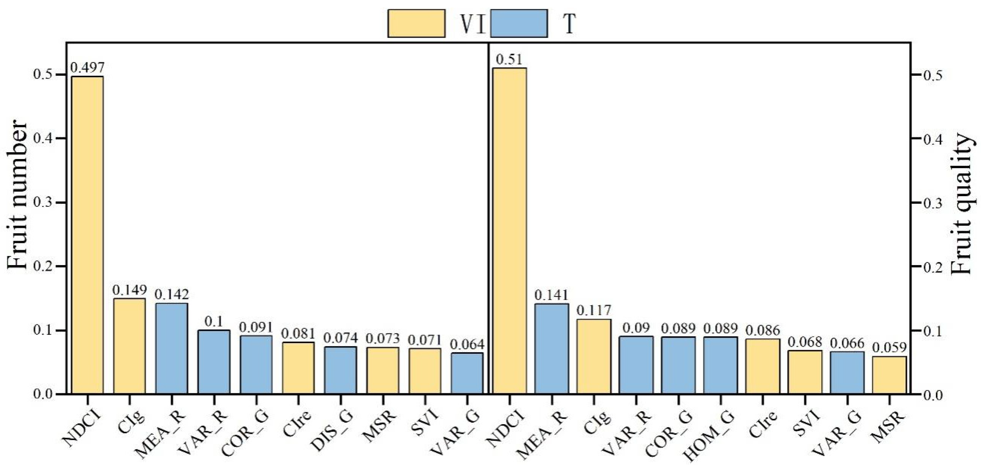
3.1. Screening of Vegetation Indices and Texture Features

According to the screening results in Figure 3, the high-weight vegetation indices and the texture features were quantitatively identical. Regarding the species, the high-weight vegetation indices were also the same, while four of the high-weight texture features were the same. For fruit number, the gain values of the vegetation indices ranged from 0.497 to 0.071, and the gain values of the texture features ranged from 0.064 to 0.142. For fruit quality, the gain values of vegetation indices ranged from 0.059 to 0.510, and the gain values of texture features ranged from 0.066 to 0.141. Meanwhile, both the NDCI vegetation index and the MEA_R texture feature contributed the most to the number and quality of citrus fruits.

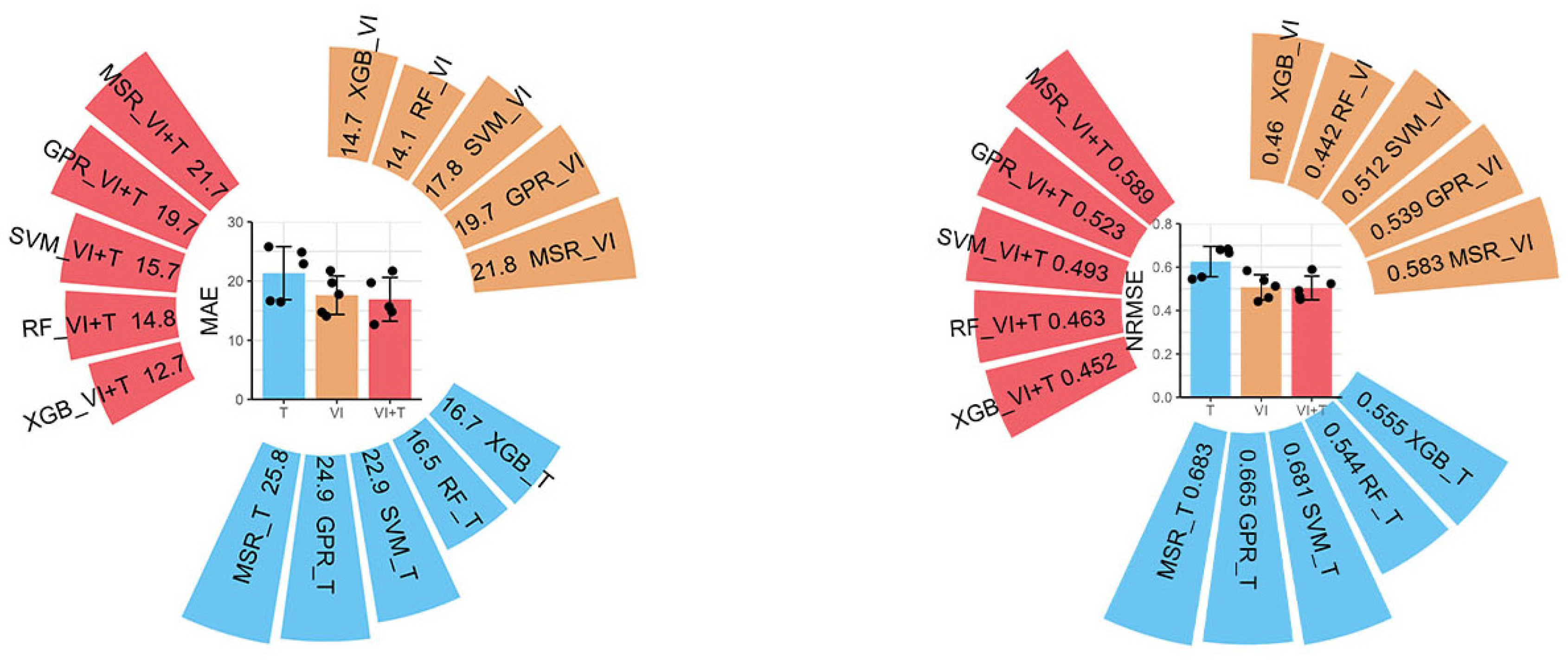
3.2. Using Machine Learning Models to Predict Citrus Fruit Yield

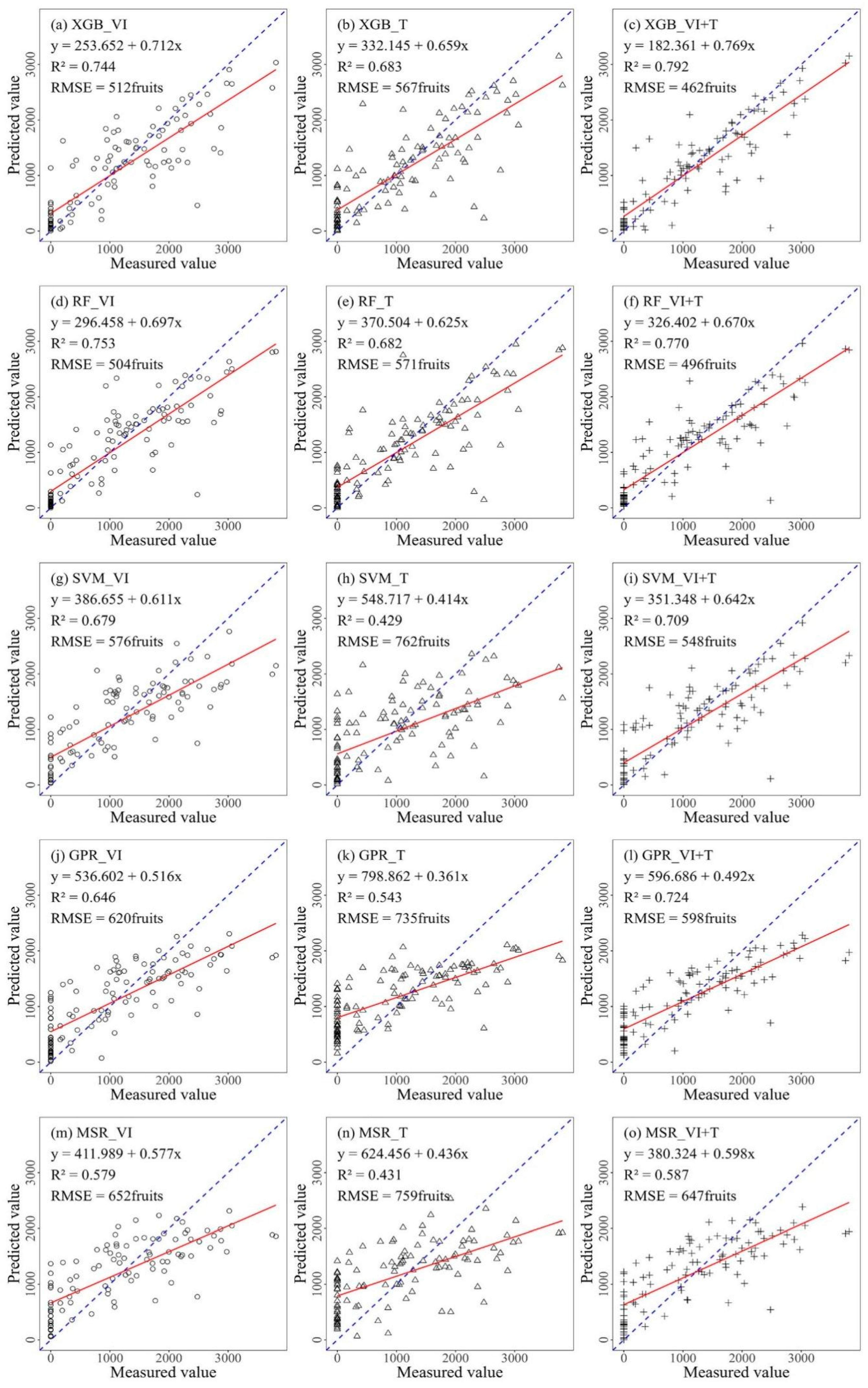
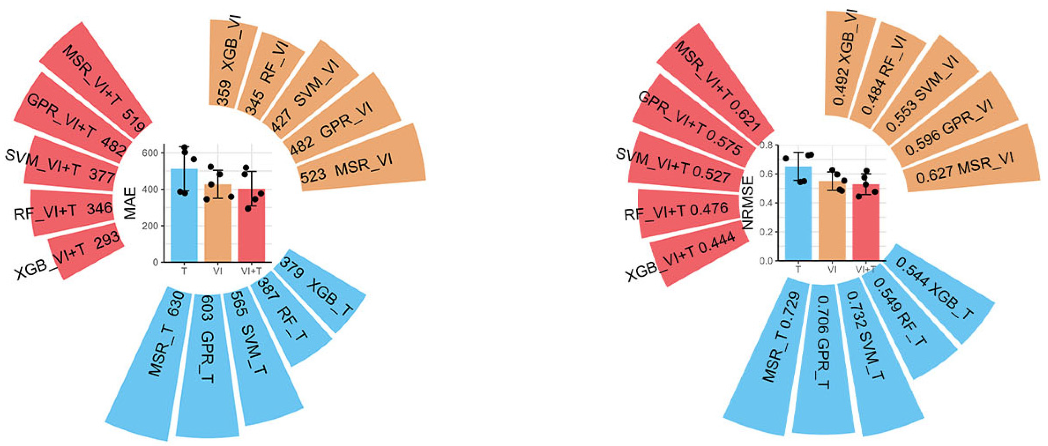
3.2.1. Prediction Models of Citrus Fruit Number in Three Combinations

To assess the predictive accuracy of five machine learning models for citrus fruit number, we utilized three input combinations: vegetation indices alone (the VI combination), texture features alone (the T combination), and a combination of both (the VI + T combination). Figure 4 presents the scatter plots of the model predictive results. Under the VI combination, the order of the model prediction performance from high to low was RF > XGB > SVM > GPR > MSR. The RF model had the best performance, and its R², RMSE, MAE, and NRMSE values were 0.753, 504 fruits, 345 fruits, and 0.484, respectively. Under the T combination, the order of model prediction performance from high to low was XGB > RF > GPR > SVM > MSR. The XGB model had the best performance, and its R², RMSE, MAE, and NRMSE values were 0.683, 567 fruits, 379 fruits, and 0.544, respectively. Under the VI + T combination, the order of model prediction performance from high to low was > RF > GPR > SVM > MSR. The XGB model had the best performance, and its R², RMSE, MAE, and NRMSE values were 0.792, 462 fruits, 293 fruits, and 0.444, respectively. When considering individual model performance, the XGB model had the best performance under the VI + T combination and its R² value reached 0.792, which is 6.5% higher than that under the VI combination and 16.0% higher than that under the T combination. The RMSE value was 462 fruits, which is 9.8% lower than that under the VI combination and 18.5% lower than that under the T combination. The rest of the models, similarly, had the largest R² values and the smallest RMSE values for the VI + T combination. In general, each model under the VI + T combination was less discrete than the other two combinations. The XGB and RF models had a similar performance and significantly outperformed the other three models. According to the MAE and NRMSE values shown in Figure 5, the MAE and NRMSE values of the XGB and RF models under the VI combination and the T combination were not much different and were significantly smaller than those of the other three models. However, under the VI + T combination, the MAE and NRMSE values of the XGB model were smaller than those of the RF model. Meanwhile, the MAE and NRMSE values of the SVM, GPR, and MSR models under the three combinations showed a trend toward increasing in turn. In addition, the histogram of the ring center in Figure 5 reveals that the comprehensive performance of all models under the VI + T combination was better than that of the VI or T variables alone. In summary, the XGB model had the best performance in predicting the number of citrus fruits under the VI + T combination, indicating that the T combination can improve the prediction accuracy of the model. The model using VI alone was superior to the model using T alone in terms of prediction accuracy, a phenomenon which may be related to the higher information content of VI in identifying and counting fruits.

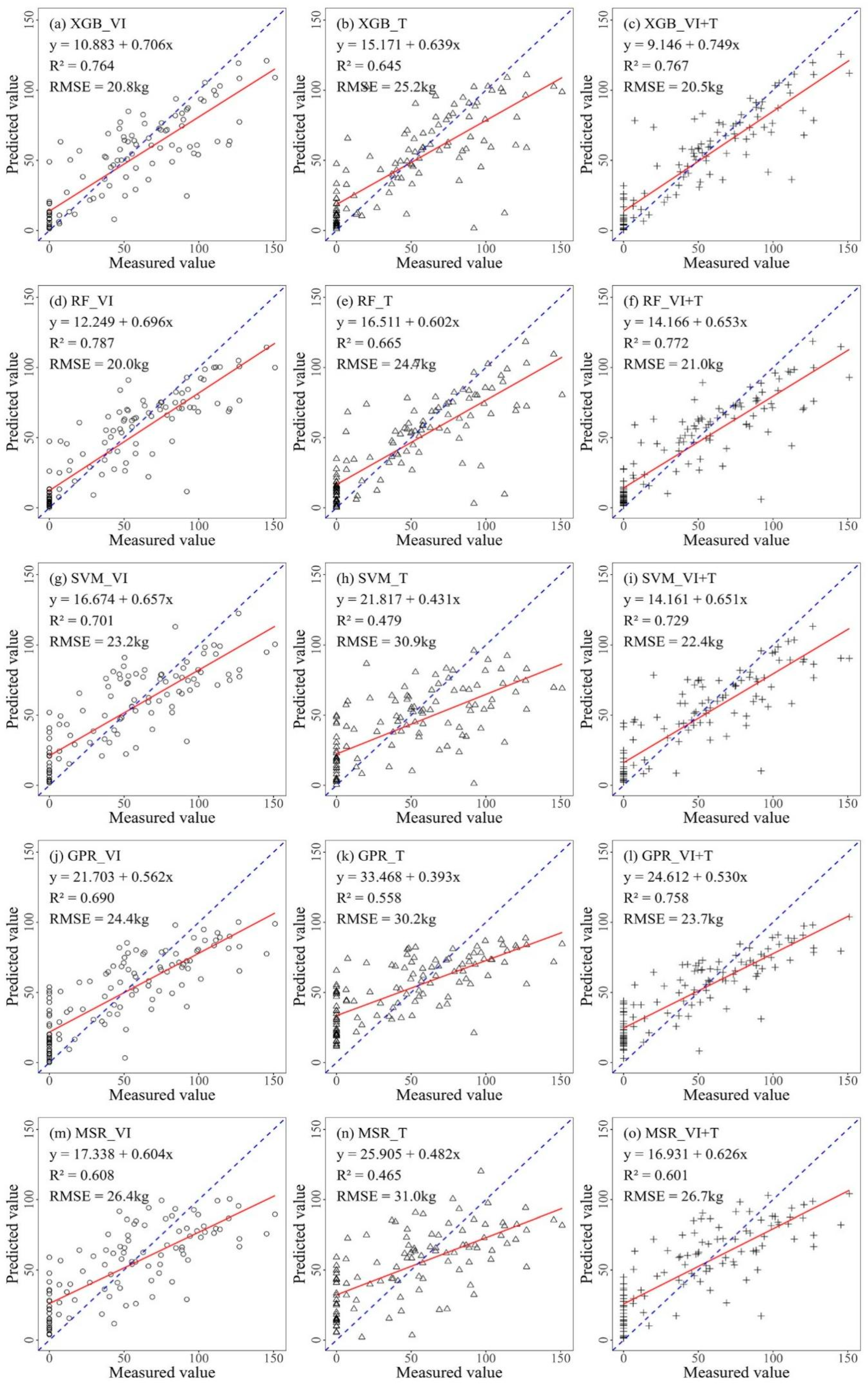
3.2.2. Prediction Models of Citrus Fruit Quality in Three Combinations

To assess the predictive accuracy of five machine learning models for citrus fruit quality, we utilized three input combinations: vegetation indices alone, texture features alone, and a combination of both. Figure 6 presents the scatter plots of the model predictive results. Under the VI combination, the order of model prediction performance from high to low was RF > XGB > SVM > GPR > MSR. The RF model had the best performance, and its R², RMSE, MAE, and NRMSE values were 0.787, 20.0 kg, 14.1 kg, and 0.442, respectively. Under the T combination, the order of model prediction performance from high to low was RF > XGB > GPR > SVM > MSR. The RF model had the best performance, and its R², RMSE, MAE, and NRMSE values were 0.665, 24.7 kg, 16.5 kg, and 0.544, respectively. Under the VI + T combination, the prediction performance of the XGB and RF models was not much different and was better than that of the other three models. The order of the other three models from high to low was GPR > SVM > MSR. The R² value of the XGB model performance was smaller than that of the RF model, but the RMSE, MAE, and NRMSE values were smaller than those of the RF model. When considering individual model performance, the RF model had the best performance under the VI combination, and its R² value reached 0.787, which is 18.3% higher than that under the T combination and 1.9% higher than that under the VI + T combination; the RMSE value was 20.0, which is 19.0% lower than that under the T combination and 4.8% lower than that under the VI + T combination. Compared with the RF model, the rest of the models, except for the MSR model, had the largest R² value and the smallest RMSE value under the VI + T combination. In general, each model under the VI + T combination was less discrete than under the T combination but similar to the VI combination. The XGB and RF models had a similar performance and significantly outperformed the other three models. According to the MAE and NRMSE values shown in Figure 7, the MAE and NRMSE values of the XGB and RF models under the VI combination and the T combination were not much different and were significantly smaller than those of the other three models. However, under the VI + T combination, the MAE value of the XGB model was smaller than that of the RF model, and the NRMSE value was still not much different. Meanwhile, the MAE and NRMSE values of the SVM, GPR, and MSR models under the three combinations revealed a trend toward increasing in turn. In addition, the histogram of the ring center in Figure 7 shows that the comprehensive performance of all models under the VI + T combination was better than that of the VI or T variables alone. In summary, the RF model had the best performance in predicting citrus fruit quality under the VI combination, indicating that VI and T may contain repetitive information. It could result in a poor performance by the RF model due to increased complexity. The model using VI alone was superior to the model using T alone in terms of prediction accuracy, a phenomenon which indicates that the VI model can more effectively capture the key factors affecting citrus fruit quality.

3.3. Using CPSO-Coupled XGB and SVM Models to Predict Citrus Fruit Yield

To further explore the most suitable machine learning model for predicting citrus yield, the particle swarm optimization algorithm in the meta-heuristic algorithm was improved. Through the joint coding method, i.e., using decimal coding to optimize the parameters of the machine learning model and, at the same time, using binary coding to select the input features, the machine learning model’s feature screening and parameter optimization can be carried out simultaneously. Considering the simplicity of the model input factors, we set the input factors to 3–9. The prediction results of the CPSO-coupled XGB and SVM models are shown in

Table 5. Statistical indicators of citrus fruit number predicted by CPSO-coupled models.

Model	Number of Input	Input Factors	R2	RMSE (Fruits)	MAE (Fruits)	NRMSE
CPSO-XGB1	3	CIg, NDCI, COR_RE	0.819	432	230	0.415
CPSO-XGB2	4	CIg, NDCI, MEA_G, COR_RE	0.803	451	300	0.434
CPSO-XGB3	5	CIg, NDCI, COR_G, SEM_NIR, MEA_RE	0.853	387	197	0.372
CPSO-XGB4	6	CIg, NDCI, SEM_G, MEA_RE, HOM_RE, COR_R	0.811	441	244	0.424
CPSO-XGB5	7	CIg, NDCI, SEM_G, ENT_NIR, MEA_RE, VAR_RE, SEM_RE	0.850	395	213	0.380
CPSO-XGB6	8	CIg, NDCI, COR_G, MEA_NIR, CON_NIR, DIS_NIR, MEA_RE, ENT_RE	0.835	417	259	0.401
CPSO-XGB7	9	CIg, DVI, NDCI, MEA_G, VAR_G, COR_G, VAR_NIR, MEA_RE, DIS_R	0.816	435	225	0.418
CPSO-SVM1	3	CIg, WDRVI, COR_G	0.780	474	321	0.456
CPSO-SVM2	4	NDCI, RVI, MEA_G, VAR_R	0.734	520	372	0.499
CPSO-SVM3	5	NDCI, NDVI, WDRVI, MEA_G, VAR_R	0.733	520	367	0.500
CPSO-SVM4	6	CIg, NDCI, RVI, MEA_G, VAR_R, CON_R	0.775	482	334	0.463
CPSO-SVM5	7	CIg, NDVI, MEA_G, COR_G, COR_NIR, MEA_R, VAR_R	0.825	424	266	0.408
CPSO-SVM6	8	CIg, DVI, NDCI, RDVI, MEA_G, ENT_NIR, HOM_RE, VAR_R	0.828	425	277	0.408
CPSO-SVM7	9	NDCI, NDVI, SVI, VAR_G, MEA_NIR, HOM_NIR, MEA_RE, VAR_RE, MEA_R	0.852	391	234	0.375

Note 3: The bold is the optimal combination in the group.

and

Table 6. Statistical indicators of citrus fruit quality predicted by CPSO-coupled models.

Model	Number of Input	Input Factors	R2	RMSE (kg)	MAE (kg)	NRMSE
CPSO-XGB1	3	CIg, NDCI, SEM_G	0.749	21.3	16.5	0.47
CPSO-XGB2	4	CIre, NDCI, ENT_G, SEM_G	0.83	17.8	12.7	0.392
CPSO-XGB3	5	CIg, DVI, NDCI, SEM_G, ENT_RE	0.844	17	12	0.374
CPSO-XGB4	6	CIg, DVI, NDCI, MEA_G,DIS_NIR, SEM_RE	0.878	14.8	9.3	0.326
CPSO-XGB5	7	CIg, CIre, NDCI, REDVI, ENT_RE, MEA_R, VAR_R	0.746	21.6	17.6	0.477
CPSO-XGB6	8	CIg, NDCI, REDVI, MEA_G, HOM_G, COR_G, MEA_NIR, ENT_NIR	0.867	15.6	10.2	0.344
CPSO-XGB7	9	CIg, MSR, NDCI, REDVI, HOM_G, ENT_G, DIS_RE, SEM_RE, CON_R	0.874	15.4	9.7	0.34
CPSO-SVM1	3	CIg, NDCI, COR_G	0.829	17.5	11.9	0.387
CPSO-SVM2	4	NDCI, WDRVI, MEA_G, VAR_R	0.772	20.2	14.6	0.446
CPSO-SVM3	5	MSR, NDCI, RVI, MEA_G, MEA_R	0.776	20.1	14.8	0.443
CPSO-SVM4	6	CIg, MSR, NDVI, MEA_G, MEA_R, VAR_R	0.78	19.8	14.4	0.437
CPSO-SVM5	7	MSR, NDRE, NDCI, WDRVI, MEA_G, MEA_R, CON_R	0.783	19.8	13.3	0.436
CPSO-SVM6	8	CIg, MNLI, RVI, SVI, ENT_G, SEM_NIR, MEA_R, SEM_R	0.841	17	11.2	0.375
CPSO-SVM7	9	CIg, MNLI, SVI, WDRVI, SEM_NIR, MEA_RE, HOM_RE, MEA_R, VAR_R	0.88	14.8	9.7	0.326

Note 4: The bold is the optimal combination in the group.

.

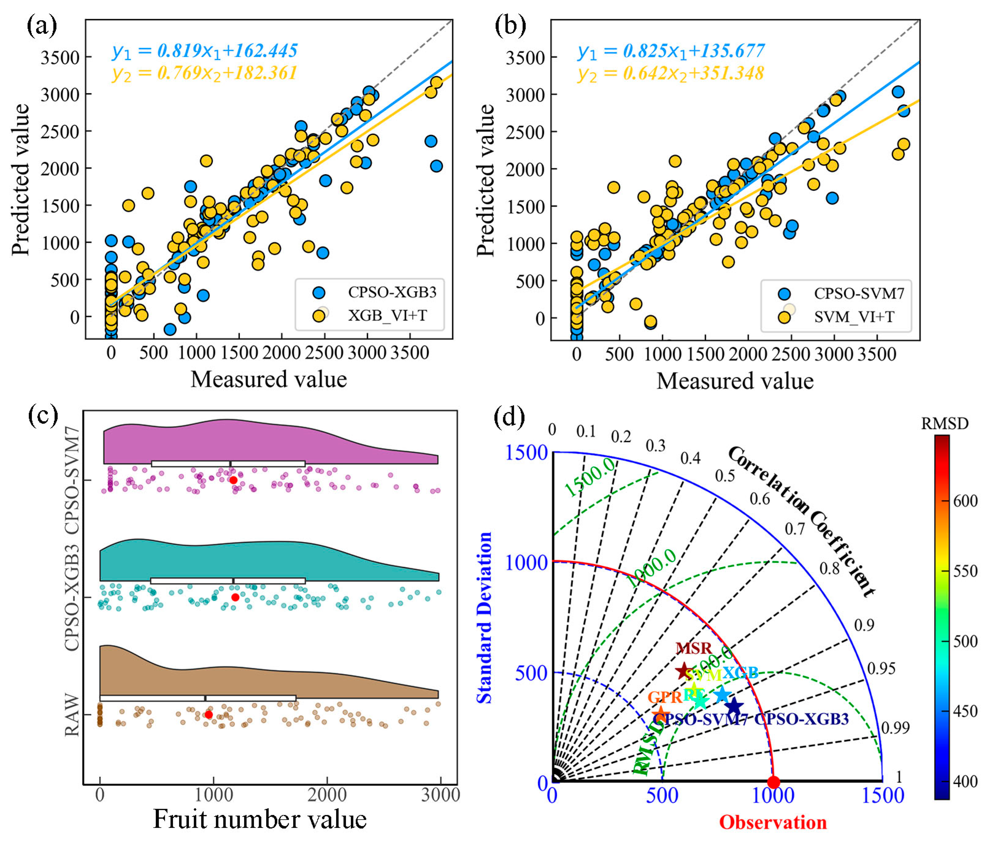
3.3.1. Comparison of CPSO-Optimized Models for Citrus Fruit Number Prediction

It can be seen from Table 5 that, for the CPSO-coupled XGB models, the CPSO-XGB3 model had the best performance, with an R² reaching 0.853, an RMSE of 387 fruits, a MAE of 197 fruits, and an NRMSE of 0.372. Compared with the CPSO-SVM3 model, the R² of the CPSO-XGB3 model increased by 16.4%, the RMSE decreased by 25.6%, the MAE decreased by 6.3%, and the NRMSE decreased by 25.6%. Compared with the XGB model under the VI + T combination in Section 3.2.1, the R² of the CPSO-XGB3 model increased by 16.4%, the RMSE decreased by 25.6%, the MAE decreased by 6.3%, and the NRMSE decreased by 25.6%. For the CPSO-coupled SVM models, the CPSO-SVM7 had the best performance, with an R² of 0.852, an RMSE of 391 fruits, a MAE of 234 fruits, and an NRMSE of 0.375. Compared with the CPSO-XGB7 model, the R² of the CPSO-SVM7 model increased by 4.4%, the RMSE decreased by 10.1%, the MAE increased by 4.0%, and the NRMSE decreased by 10.3%. Compared with the SVM model under the VI + T combination in Section 3.2.1, the R² of the CPSO-SVM7 model increased by 20.2%, the RMSE decreased by 28.6%, the MAE decreased by 37.9%, and the NRMSE decreased by 28.8%. Overall, the optimal model (CPSO-XGB3) among the CPSO-coupled XGB models was better than the optimal model (CPSO-SVM7) among the CPSO-coupled SVM models. Compared with CPSO-SVM7, the R² of CPSO-XGB3 increased by 0.1%, the RMSE decreased by 1%, the MAE decreased by 15.8%, and the NRMSE decreased by 0.8%. The NDCI and MEA_RE features were selected from the two coupled optimal models.

Figure 8a,b display that the CPSO-optimized machine learning model had a smaller dispersion than the unoptimized model. Figure 8c shows the cloud–rain map of the predicted data and the original data for the CPSO-XGB3 and CPSO-SVM7 models. The median and mean of the predicted data from the two optimized models were larger than the measured data, and the predicted data were evenly distributed. Figure 8d shows the Taylor diagram of the five machine learning models in Section 3.2.1 and the two optimal CPSO-coupled models. With respect to the standard deviation, all models were lower than the measured values. The standard deviation of the GPR model was the lowest, and the standard deviation of the two CPSO-coupled models was higher. With respect to the correlation coefficient, the correlation coefficients of the two CPSO-coupled models were greater than 0.9 and not much different. The values of the other models were lower than 0.9, among which the value of the MSR model had the smallest correlation coefficient. With respect to the RMSD, the values of the two CPSO-coupled models and the XGB and RF models were all below 500 fruits. The values of the two CPSO-coupled models were relatively low, indicating that the CPSO-optimized models had a smaller prediction error and better prediction results compared to the unoptimized machine learning models.

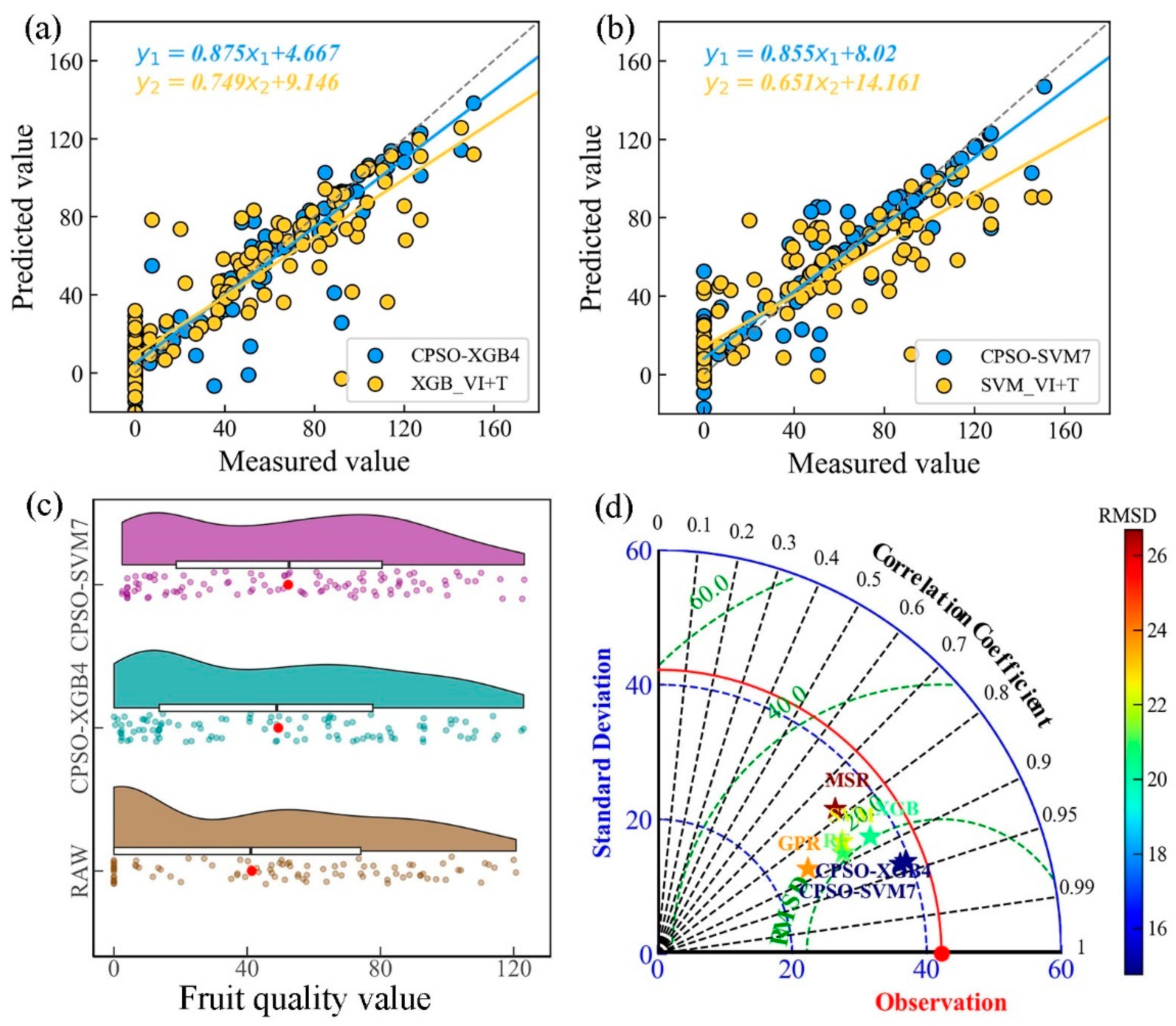
3.3.2. Comparison of CPSO-Optimized Models for Citrus Fruit Quality Prediction

It can be seen from Table 6 that, for the CPSO-coupled XGB model, the CPSO-XGB4 model had the best performance, with an R² reaching 0.878, an RMSE of 14.8 kg, a MAE of 9.3 kg, and an NRMSE of 0.326. Compared with the CPSO-SVM4 model, the R² of the CPSO-XGB4 model increased by 12.6%, the RMSE decreased by 25.3%, the MAE decreased by 35.4%, and the NRMSE decreased by 25.4%. Compared with the XGB model under the VI + T combination in Section 3.2.2, the R² of the CPSO-XGB4 model increased by 14.5%, the RMSE decreased by 27.8%, the MAE decreased by 26.8%, and the NRMSE decreased by 27.9%. For the CPSO-coupled SVM model, the CPSO-SVM7 had the best performance, with an R² of 0.88, an RMSE of 14.8 kg, a MAE of 9.7 kg, and an NRMSE of 0.326. Compared with the CPSO-XGB7 model, the R² of the CPSO-SVM7 model increased by 0.7%, the RMSE decreased by 3.9%, the MAE did not change, and the NRMSE decreased by 4.1%. Compared with the SVM model under the VI + T combination in Section 3.2.2, the R² of the CPSO-SVM7 model increased by 20.7%, the RMSE decreased by 33.9%, the MAE decreased by 38.2%, and the NRMSE decreased by 33.9%. Overall, the optimal model (CPSO-XGB4) among the CPSO-coupled XGB models and the optimal model (CPSO-SVM7) among the CPSO-coupled SVM models had the same performance in predicting fruit quality. However, the CPSO-XGB4 model required fewer input features. Compared with CPSO-XGB4, the R² of CPSO-SVM7 increased by 0.002, the MAE increased by 0.4, and the RMSE and NRMSE did not change. The CIg feature was selected from the two optimal coupled models.

Figure 9a,b display that the CPSO-optimized machine learning model had a smaller dispersion than the unoptimized model. Figure 9c shows the cloud–rain map of the predicted data and the original data for the CPSO-XGB4 and CPSO-SVM7 models. The median and mean of the predicted data from the two optimized models were larger than the measured data, and the predicted data were evenly distributed. Figure 9d shows the Taylor diagram of the five machine learning models in Section 3.2.2 and the two optimal CPSO-coupled models. With respect to the standard deviation, all models were lower than the measured value. The standard deviation of the two CPSO-coupled models was higher, and the value of CPSO-XGB4 was greater than that of CPSO-SVM7. From the correlation coefficient, the correlation coefficients of the two CPSO-coupled models were close to 0.95. The values of the other models were lower than 0.9, among which the value of the MSR model was the smallest. With respect to the RMSD, the values of the two CPSO-coupled models were below 20 kg. The values of the other models were greater than 20 kg, indicating that the CPSO-optimized models had a lower prediction error and better prediction results compared to the unoptimized machine learning models.

3.4. Analysis of Input Features

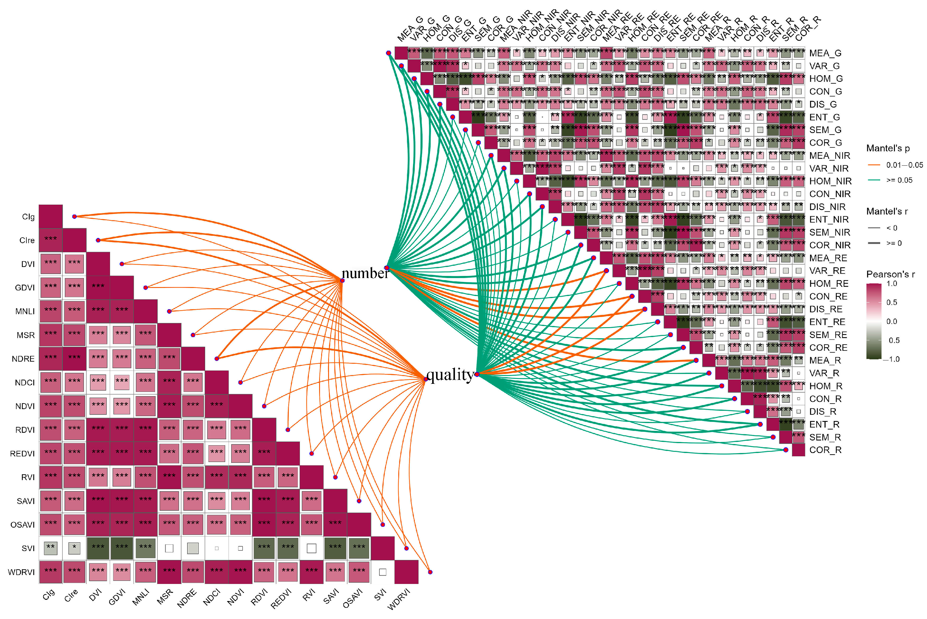
3.4.1. Correlation Analysis

In this study, a mantel analysis was performed between the model input features and the citrus fruit number and quality. Figure 10 displays the analysis results. From the left half of the figure, except for the SVI index, which shows negative correlations with other vegetation indices, all the remaining vegetation indices demonstrated obvious positive correlations with good significance levels. Most of the correlations between the vegetation indices and the citrus number were negative, except for CIg, CIre, and NDRE. Most of the correlations between the vegetation indices and the citrus quality showed negative correlations, except for CIre and NDRE. In addition, the significance of the correlations was always in the range of 0.01–0.05. From the right half of the figure, it can be seen that the correlations among the 32 texture features in the multispectral bands were both positive and negative, with varying degrees of significance levels. The correlations between the 32 texture features and the citrus number and quality were both positive and negative, and most of the significance values were greater than or equal to 0.05. The correlation significance of only VAR_RE, CON_RE, DIS_RE, and MEA_R in relation to the citrus number was in the range of 0.01–0.05, while the correlation significance of only VAR_RE, CON_RE, and DIS_RE in relation to citrus quality was in the range of 0.01–0.05.

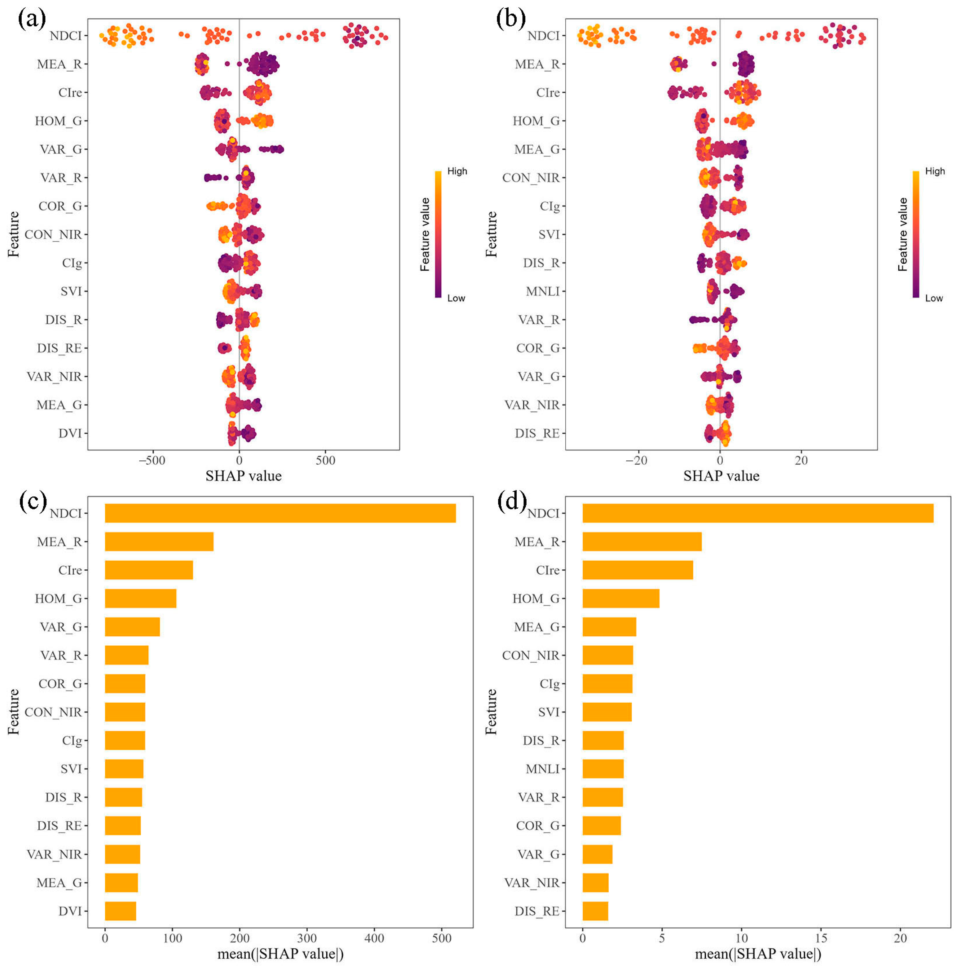
3.4.2. SHAP Analysis

Based on the analysis in Section 3.2, we found that the XGB model was the optimal model for predicting citrus fruit number and performed better for predicting citrus fruit quality. Secondly, the data distribution of fruit number and quality had more variability. To more accurately explore the influence of 16 vegetation indices and 32 texture features on the number and quality of citrus fruits per plant, we used the SHAP method to analyze the interpretability of the feature variables entered into the XGB model.

Each point in the distribution graph is a feature value and a SHAP value. The SHAP value is zero as the intermediate dividing line. The sample on the left side shows a negative effect, and the sample on the right side shows a positive effect. Color represents the level of the corresponding feature value. In Figure 11a, smaller values of NDCI had a greater positive impact on the citrus fruit number prediction model; larger values had a greater negative impact on the model. The fluctuation range of the SHAP values of the remaining input features was between −500 and 500. Similarly, in Figure 11b, the NDCI showed the same pattern, with fluctuations in the remaining input feature SHAP values ranging from −20 to 20. The average absolute value of each feature in the feature importance graph in all samples was regarded as the global importance of the feature. It can be seen from Figure 11c,d that the NDCI vegetation index was significantly better than the other 14 features. The NDCI vegetation index had a significant effect on the prediction model of fruit number and quality, and the average absolute SHAP values were greater than 500 and 20, respectively. Section 3.1 utilized the important function of the XGB model to screen features, and it was similarly found that the top three important features of the model for predicting the number and quality of fruits were NDCI, CIre, and MEA_R. This not only showed that NDCI, CIre, and MEA_R had a significant impact on estimating the number and quality of fruits, but also proved the rationality of the XGB model algorithm for calculating the importance of features when constructing the model.

4. Discussion

4.1. Comparison of Different Machine Learning Models

Different machine learning models have different basic concepts and algorithm mechanisms, so each model has different advantages and disadvantages and is suited to specific application scenarios [48]. This study focused on the differences among the five machine learning models of XGB, RF, SVM, GPR, and MSR for citrus yield prediction. The results show that the XGB and RF models performed outstandingly. The main reason is that these two methods belong to ensemble learning, which is integrated into the ideas of boosting and bagging, respectively. Specifically, the XGB model is similar to an iterative optimization process, which achieves a higher prediction accuracy of the model by gradually constructing multiple weak learners and using the residuals of the previous learner as the training objective of the next learner, thus gradually correcting the prediction error to get a strong learner. However, it requires many hyperparameters and is troublesome to adjust. The RF model, on the other hand, is similar to multiple independent experiments to reduce random errors. It constructs multiple decision trees by randomly selecting features and data samples and aggregates the prediction results of these trees to reduce the dependence on specific data and improve the accuracy of prediction. However, its integrated nature makes the decisions of individual trees difficult to interpret. In contrast, SVM maximizes the classification accuracy of a sample by finding the optimal decision boundary and solves the nonlinearity problem by mapping the kernel function to a high-dimensional space. Although it performs well on small-sample datasets, it has a higher computational complexity and longer training time when dealing with large-scale datasets. GPR, as a probability-based regression method, is able to quantify the prediction results, give confidence intervals for the predicted values, and provide an estimate of the prediction uncertainty, but it is computationally costly and noise-sensitive when dealing with high-dimensional data. MSR, by progressively screening the variables, it effectively selects the variable that has the greatest effect on the dependent variable to build the optimal regression equation, which is interpretive for multicollinearity problems but may not perform well in dealing with nonlinear relationships and complex features. For the prediction of citrus fruit number and quality, such a prediction usually involves complex interactions and nonlinear relationships among multiple variables. The XGB and RF models are superior to other models in terms of their prediction effect because of their flexibility and ability to capture feature interactions and the advantages of combining multiple learners. This conclusion is similar to the research results of Pei et al. [49] to estimate the water status of cotton canopy and Guimarães et al. [50] to predict stomatal conductance in almond orchards. However, in this study, the R² values of the XGB and RF models in citrus yield prediction were lower than 0.8. This may be because citrus is a perennial evergreen fruit tree with a large and thick canopy formed by less deciduous leaves throughout the year [51], making it difficult for the UAV to accurately obtain canopy spectral information, resulting in low modeling accuracy.

4.2. The Prediction Advantage of Vegetation Indices Combined with Texture Features

At harvest time, citrus is at the fruit maturity stage. The canopy coverage of the fruit trees in citrus orchards is large, which may lead to the easy saturation of the vegetation indices, i.e., the values of the vegetation indices no longer change significantly after a certain vegetation density [52]. Therefore, this study added texture features for comparison. The results show that the accuracy of the five machine learning models combined with texture features was overall better than that of the models based only on vegetation indices as input. This conclusion is consistent with the results of Kwak et al. [53], who used UAV images for crop classification, and Dhakal et al. [54], who estimated the aboveground biomass of oats. Since the vegetation indices fused with texture features contain both spectral and texture information of UAV images, they can essentially explain and construct the growth of citrus from a two-dimensional perspective. Therefore, the accuracy of the model is improved. The gray level co-occurrence matrix (GLCM) effectively describes the image texture features by analyzing the gray level joint probability of pixel pairs at a specific distance and direction in the image [55]. However, the large number of features extracted by GLCM not only increased the complexity of model fitting, but also increased the difficulty of finding the optimal model. In addition, most of the single texture features were not significantly correlated with the number and quality of citrus fruits. Future studies may consider normalizing texture features using vegetation index construction methods [56] to enhance their correlation with fruit yield. In this study, the importance function of the XGB model was used to rank the importance of 16 vegetation indices and 32 texture features. The results show that the most important vegetation index in citrus yield prediction was NDCI, and the most important texture feature was MEA_R. The health and photosynthetic efficiency of trees typically influence citrus yield. Therefore, NDCI, as an indicator of chlorophyll content, is closely related to plant health and growth vigor, both of which can be directly related to citrus yield [30]. MEA_R is the texture mean of the red band, which not only reflects the surface structure of vegetation but is also related to chlorophyll absorption. The two are often related to yield, a fact which is crucial for yield prediction [57]. Also, the SHAP analysis in this paper proved this point. In future research, the characteristics of plant height and crown area should be added to the prediction of the model, and the citrus yield should be predicted from more dimensions to improve the accuracy of the model.

4.3. The Prediction Advantage of CPSO-Coupled Models

The simulation accuracy of the machine learning model algorithm is affected by the parameters of the model and the feature selection of the datasets. The optimization of model parameters can adjust the internal working mechanism of the algorithm to make it more suitable for the distribution of data and to prevent the risk of overfitting [58]. Feature selection can reduce computational time, improve model accuracy, and help better understand the model by removing irrelevant and redundant features [59]. Because the traditional feature screening method selects many features of the optimal combination and the parameter optimization of machine learning requires a lot of trial calculations, this paper proposes an improved meta-heuristic optimization algorithm. This method encodes and optimizes the parameters of the machine learning model and the input features simultaneously through a hybrid coding approach. Finally, the appropriate prediction model parameters and feature input combinations for the number and quality of citrus fruits were obtained. The CPSO-coupled model effectively reduces the collinearity of input features and the risk of model overfitting by selecting ideal model parameters and using as few features as possible. The results show that the optimal CPSO-coupled model (CPSO-XGB3) reduced the input features from 48 to five to predict the citrus fruit number. In the prediction of citrus fruit quality, the optimal CPSO-coupled model (CPSO-XGB4) reduced the input features from 48 to six. At the same time, these two optimal models had higher accuracy. The successful application of this method provides a powerful tool for accurate prediction and management in the field of agriculture, and also provides new ideas for complex prediction problems in other fields.

5. Conclusions

Based on the multispectral images of the UAV, this study investigates the potential of vegetation indices combined with texture features to predict citrus yield and confirms the superiority of the machine learning model coupled with the CPSO method. Specifically, the combination of vegetation indices and texture features can improve the predictive performance of the model compared to a single feature input. For predicting citrus fruit number, the XGB model performed best under the VI + T combination. For predicting citrus fruit quality, the RF model performed optimally when only the vegetation indices were used. In addition, the CPSO method was introduced in this study to optimize the XGB and SVM models. The results show that the CPSO-optimized models had significant improvements in predicting the number and quality of citrus fruits, with the CPSO-XGB model performing the best. For predicting citrus fruit number, the CPSO-XGB model had the highest accuracy when the input features were five. Compared with the XGB model under the VI + T combination, the R² increased by 16.4% and the RMSE decreased by 25.6%. For predicting citrus fruit quality, the CPSO-XGB model had the highest accuracy when the input features were six. Compared with the XGB model under the VI + T combination, the R² increased by 14.5% and the RMSE decreased by 27.8%. In summary, the UAV inversion technology combined with spectral indices and texture features can provide an economical, rapid, and effective method for citrus yield prediction. Meanwhile, it can also offer a theoretical basis for predicting large-scale yield of citrus orchards in the future.

The limitation of this study is the specific geographic and climatic environment, and the generalization ability of the model needs to be validated in different regions and conditions. Therefore, in future studies, the modeling can be combined with local soil and climatic conditions. In addition, we hope to evaluate the ability of the CPSO-XGB model in predicting citrus leaf area index, leaf nitrogen content, and soil water content.

References

1. Liu, Y.; Heying, E.; Tanumihardjo, S.A. History, global distribution, and nutritional importance of citrus fruits. Compr. Rev. Food Sci. Saf. 2012, 11, 530–545. [Google Scholar] [CrossRef]
2. Saini, R.K.; Ranjit, A.; Sharma, K.; Prasad, P.; Shang, X.; Gowda, K.G.M.; Keum, Y.S. Bioactive compounds of citrus fruits: A review of composition and health benefits of carotenoids, flavonoids, limonoids, and terpenes. Antioxidants 2022, 11, 239. [Google Scholar] [CrossRef]
3. Tang, Y.; Liu, X.; Yang, H.; Xu, C.; Wang, S.; Hu, Z. Comparison of fruit mastication trait among different citrus reticulata blanco cv. kinokuni varieties (lines). J. South. Agric. 2023, 54, 3657–3664. [Google Scholar]
4. Godfray, H.C.J.; Beddington, J.R.; Crute, I.R.; Haddad, L.; Lawrence, D.; Muir, J.F.; Pretty, J.; Robinson, S.; Thomas, S.M.; Toulmin, C. Food Security: The Challenge of Feeding 9 Billion People. Science 2010, 327, 812–818. [Google Scholar] [CrossRef] [PubMed]
5. Guebsi, R.; Mami, S.; Chokmani, K. Drones in Precision Agriculture: A Comprehensive Review of Applications, Technologies, and Challenges. Drones 2024, 8, 686. [Google Scholar] [CrossRef]
6. Zhao, X.; Zhao, Z.; Zhao, F.; Liu, J.; Li, Z.; Wang, X.; Gao, Y. An estimation of the leaf nitrogen content of apple tree canopies based on multispectral unmanned aerial vehicle imagery and machine learning methods. Agronomy 2024, 14, 552. [Google Scholar] [CrossRef]
7. Zhang, Y.; Ta, N.; Guo, S.; Chen, Q.; Zhao, L.; Li, F.; Chang, Q. Combining spectral and textural information from UAV RGB images for leaf area index monitoring in kiwifruit orchard. Remote Sens. 2022, 14, 1063. [Google Scholar] [CrossRef]
8. Maimaitijiang, M.; Sagan, V.; Sidike, P.; Hartling, S.; Esposito, F.; Fritschi, F.B. Soybean yield prediction from UAV using multimodal data fusion and deep learning. Remote Sens. Environ. 2020, 237, 111599. [Google Scholar] [CrossRef]
9. Sanches, G.M.; Duft, D.G.; Kölln, O.T.; Luciano, A.C.D.S.; De Castro, S.G.Q.; Okuno, F.M.; Franco, H.C.J. The potential for RGB images obtained using unmanned aerial vehicle to assess and predict yield in sugarcane fields. Int. J. Remote Sens. 2018, 39, 5402–5414. [Google Scholar] [CrossRef]
10. Taşan, S.; Cemek, B.; Taşan, M.; Cantürk, A. Estimation of eggplant yield with machine learning methods using spectral vegetation indices. Comput. Electron. Agric. 2022, 202, 107367. [Google Scholar] [CrossRef]
11. Lukas, V.; Huňady, I.; Kintl, A.; Mezera, J.; Hammerschmiedt, T.; Sobotková, J.; Brtnický, M.; Elbl, J. Using UAV to identify the optimal vegetation index for yield prediction of oil seed rape (Brassica napus L.) at the flowering stage. Remote Sens. 2022, 14, 4953. [Google Scholar] [CrossRef]
12. Van Beek, J.; Tits, L.; Somers, B.; Deckers, T.; Verjans, W.; Bylemans, D.; Janssens, P.; Coppin, P. Temporal dependency of yield and quality estimation through spectral vegetation indices in pear orchards. Remote Sens. 2015, 7, 9886–9903. [Google Scholar] [CrossRef]
13. Rotili, D.H.; de Voil, P.; Eyre, J.; Serafin, L.; Aisthorpe, D.; Maddonni, G.Á.; Rodríguez, D. Untangling genotype x management interactions in multi-environment on-farm experimentation. Field Crop Res. 2020, 255, 107900. [Google Scholar] [CrossRef]
14. Khaki, S.; Wang, L.; Archontoulis, S.V. A CNN-RNN framework for crop yield prediction. Front. Plant Sci. 2019, 10, 1750. [Google Scholar] [CrossRef] [PubMed]
15. Chen, R.Q.; Zhang, C.J.; Xu, B.; Zhu, Y.; Zhao, F.; Han, S.; Yang, G.; Yang, H. Predicting individual apple tree yield using UAV multi-source remote sensing data and ensemble learning. Comput. Electron. Agric. 2022, 201, 107275. [Google Scholar] [CrossRef]
16. Rahman, M.M.; Robson, A.; Bristow, M. Exploring the potential of high resolution WorldView-3 imagery for estimating yield of mango. Remote Sens. 2018, 10, 1866. [Google Scholar] [CrossRef]
17. Kang, Y.; Wang, Y.; Fan, Y.; Wu, H.; Zhang, Y.; Yuan, B.; Li, H.; Wang, S.; Li, Z. Wheat yield estimation based on unmanned aerial vehicle multispectral images and texture feature indices. Agriculture 2024, 14, 167. [Google Scholar] [CrossRef]
18. Zhang, J.; Cheng, J.; Liu, C.; Wu, Q.; Xiong, S.; Yang, H.; Chang, S.; Fu, Y.; Yang, M.; Zhang, S.; et al. Enhanced crop leaf area index estimation via random forest regression: Bayesian optimization and feature selection approach. Remote Sens. 2024, 16, 3917. [Google Scholar] [CrossRef]
19. Wei, L.; Huang, C.; Zhong, Y.; Wang, Z.; Hu, X.; Lin, L. Inland waters suspended solids concentration retrieval based on PSO-LSSVM for UAV-borne hyperspectral remote sensing imagery. Remote Sens. 2019, 11, 1455. [Google Scholar] [CrossRef]
20. Zeng, L.; Peng, G.; Meng, R.; Man, J.; Li, W.; Xu, B.; Lv, Z.; Sun, R. Wheat yield prediction based on unmanned aerial vehicles-collected red-green-blue imagery. Remote Sens. 2021, 13, 2937. [Google Scholar] [CrossRef]
21. Olson, D.; Chatterjee, A.; Franzen, D.W.; Day, S.S. Relationship of Drone-Based Vegetation Indices with Corn and Sugarbeet Yields. Agron. J. 2019, 111, 2545–2557. [Google Scholar] [CrossRef]
22. Bellis, E.S.; Hashem, A.A.; Causey, J.L.; Runkle, B.R.K.; Moreno-García, B.; Burns, B.W.; Green, V.S.; Burcham, T.N.; Reba, M.L.; Huang, X. Detecting Intra-Field Variation in Rice Yield With Unmanned Aerial Vehicle Imagery and Deep Learning. Front. Plant Sci. 2022, 13, 716506. [Google Scholar] [CrossRef] [PubMed]
23. Murray, H.; Lucieer, A.; Williams, R. Texture-based classification of sub-Antarctic vegetation communities on Heard Island. Int. J. Appl. Earth Obs. 2010, 12, 138–149. [Google Scholar] [CrossRef]
24. Kelcey, J.; Lucieer, A. Sensor correction and radiometric calibration of a 6-band multispectral imaging sensor for UAV remote sensing. Int. Arch. Photogramm. Remote Sens. Spat. Inf. Sci. 2012, 39, 393–398. [Google Scholar] [CrossRef]
25. Gitelson, A.A.; Viña, A.; Ciganda, V.; Rundquist, D.C.; Arkebauer, T.J. Remote estimation of canopy chlorophyll content in crops. Geophys. Res. Lett. 2005, 32, L08403. [Google Scholar] [CrossRef]
26. Tucker, C.J. Red and photographic infrared linear combinations for monitoring vegetation. Remote Sens. Environ. 1979, 8, 127–150. [Google Scholar] [CrossRef]
27. Gong, P.; Pu, R.L.; Biging, G.S.; Larrieu, M.R. Estimation of forest leaf area index using vegetation indices derived from hyperion hyperspectral data. Ieee T. Geosci. Remote 2003, 41, 1355–1362. [Google Scholar] [CrossRef]
28. Chen, J.M. Evaluation of vegetation indices and a modified simple ratio for boreal applications. Can. J. Remote Sens. 2014, 22, 229–242. [Google Scholar] [CrossRef]
29. Peng, Y.; Gitelson, A.A. Remote estimation of gross primary productivity in soybean and maize based on total crop chlorophyll content. Remote Sens. Environ. 2012, 117, 440–448. [Google Scholar] [CrossRef]
30. Mishra, S.; Mishra, D.R. Normalized difference chlorophyll index:a novel model for remote estimation of chlorophyll-a concentration in turbid productive waters. Remote Sens. Environ. 2012, 117, 394–406. [Google Scholar] [CrossRef]
31. Liu, H.Q.; Huete, A. A feedback based modification of the NDVI to minimize canopy background and atmospheric noise. IEEE T. Geosci. Remote 1995, 33, 457–465. [Google Scholar] [CrossRef]
32. Roujean, J.L.; Breon, F.M. Estimating PAR absorbed by vegetation from bidirectional reflectance measurements. Remote Sens. Environ. 1995, 51, 375–384. [Google Scholar] [CrossRef]
33. Cao, Q.; Miao, Y.X.; Wang, H.Y.; Huang, S.; Cheng, S.; Khosla, R.; Jiang, R. Non-destructive estimation of rice plant nitrogen status with crop circle multispectral active canopy sensor. Field Crop Res. 2013, 154, 133–144. [Google Scholar] [CrossRef]
34. Birth, G.S.; McVey, G.R. Measuring the color of growing turf with a reflectance spectrophotometer. Agron. J. 1968, 60, 640–643. [Google Scholar] [CrossRef]
35. Huete, A.R. A soil-adjusted vegetation index (SAVI). Remote Sens. Environ. 1988, 25, 295–309. [Google Scholar] [CrossRef]
36. Rondeaux, G.; Steven, M.; Baret, F. Optimization of soil-adjusted vegetation indices. Remote Sens. Environ. 1996, 55, 95–107. [Google Scholar] [CrossRef]
37. Perry, J.C.R.; Lautenschlager, L.F. Functional equivalence of spectral vegetation indices. Remote Sens. Environ. 1984, 14, 169–182. [Google Scholar] [CrossRef]
38. Gitelson, A.A. Wide dynamic range vegetation index for remote quantification of biophysical characteristics of vegetation. J. Plant Physiol. 2004, 161, 165–173. [Google Scholar] [CrossRef] [PubMed]
39. Haralick, R.M.; Shanmugam, K.; Dinstein, I. Textural Features for Image Classification. IEEE T. Syst. Man Cybern. 1973, 6, 610–621. [Google Scholar] [CrossRef]
40. Chen, T.; Guestrin, C. XGBoost. In Proceedings of the 22nd ACM SIGKDD International Conference on Knowledge Discovery and Data Mining, San Francisco, CA, USA, 13–17 August 2016; pp. 785–794. [Google Scholar]
41. Breiman, L. Random Forests. Mach. Learn. 2001, 45, 5–32. [Google Scholar] [CrossRef]
42. Vapnik, V.; Izmailov, R. Knowledge transfer in SVM and neural networks. Ann. Math. Artif. Intel. 2017, 81, 3–19. [Google Scholar] [CrossRef]
43. Wang, J. An intuitive tutorial to gaussian process regression. Comput. Sci. Eng. 2023, 25, 4–11. [Google Scholar] [CrossRef]
44. Liu, Y.; Heuvelink, G.B.M.; Bai, Z.; He, P.; Xu, X.; Ding, W.; Huang, S. Analysis of spatio-temporal variation of crop yield in China using stepwise multiple linear regression. Field Crop Res. 2021, 264, 108098. [Google Scholar] [CrossRef]
45. Kennedy, J.; Eberhart, R. Particle swarm optimization. In Proceedings of the ICNN’95-International Conference on Neural Networks, Perth, Australia, 27 November—1 December 1995; pp. 1942–1948. [Google Scholar]
46. Mojtaba Ahmadieh, K.; Mohammad, T.; Mahdi Aliyari, S. A novel binary particle swarm optimization. In Proceedings of the 2007 Mediterranean Conference on Control & Automation, Athens, Greece, 27–29 June 2007; pp. 1–6. [Google Scholar]
47. Lundberg, S.M.; Lee, S.I. A unified approach to interpreting model predictions. In Proceedings of the 31st International Conference on Neural Information Processing Systems, Long Beach, CA, USA, 4–9 December 2017; pp. 4768–4777. [Google Scholar]
48. Huang, J.-C.; Ko, K.-M.; Shu, M.-H.; Hsu, B.-M. Application and comparison of several machine learning algorithms and their integration models in regression problems. Neural Comput. Appl. 2019, 32, 5461–5469. [Google Scholar] [CrossRef]
49. Pei, S.; Dai, Y.; Bai, Z.; Li, Z.; Zhang, F.; Yin, F.; Fan, J. Improved estimation of canopy water status in cotton using vegetation indices along with textural information from UAV-based multispectral images. Comput. Electron. Agric. 2024, 224, 109176. [Google Scholar] [CrossRef]
50. Guimarães, N.; Sousa, J.J.; Couto, P.; Bento, A.; Pádua, L. Combining UAV-Based Multispectral and Thermal Infrared Data with Regression Modeling and SHAP Analysis for Predicting Stomatal Conductance in Almond Orchards. Remote Sens. 2024, 16, 1–19. [Google Scholar] [CrossRef]
51. Mo, X.; Chen, C.; Riaz, M.; Moussa, M.G.; Chen, X.; Wu, S.; Tan, Q.; Sun, X.; Zhao, X.; Shi, L.; et al. Fruit characteristics of citrus trees grown under different soil cu levels. Plants 2022, 11, 2943. [Google Scholar] [CrossRef] [PubMed]
52. Qiao, D.; Yang, J.; Bai, B.; Li, G.; Wang, J.; Li, Z.; Liu, J.; Liu, J. Non-destructive monitoring of peanut leaf area index by combing UAV spectral and textural characteristics. Remote Sens. 2024, 16, 2182. [Google Scholar] [CrossRef]
53. Kwak, G.-H.; Park, N.-W. Impact of Texture Information on Crop Classification with Machine Learning and UAV Images. Appl. Sci. 2019, 9, 643. [Google Scholar] [CrossRef]
54. Dhakal, R.; Maimaitijiang, M.; Chang, J.; Caffe, M. Utilizing Spectral, Structural and Textural Features for Estimating Oat Above-Ground Biomass Using UAV-Based Multispectral Data and Machine Learning. Sensors 2023, 23, 9708. [Google Scholar] [CrossRef] [PubMed]
55. Honeycutt, C.E.; Plotnick, R. Image analysis techniques and gray-level co-occurrence matrices (GLCM) for calculating bioturbation indices and characterizing biogenic sedimentary structures. Comput. Geosci. 2008, 34, 1461–1472. [Google Scholar] [CrossRef]
56. Yang, N.; Zhang, Z.; Zhang, J.; Guo, Y.; Yang, X.; Yu, G.; Bai, X.; Chen, J.; Chen, Y.; Shi, L.; et al. Improving estimation of maize leaf area index by combining of UAV-based multispectral and thermal infrared data: The potential of new texture index. Comput. Electron. Agric. 2023, 214, 108294. [Google Scholar] [CrossRef]
57. Zheng, H.; Cheng, T.; Zhou, M.; Li, D.; Yao, X.; Tian, Y.; Cao, W.; Zhu, Y. Improved estimation of rice aboveground biomass combining textural and spectral analysis of UAV imagery. Precis. Agric. 2018, 20, 611–629. [Google Scholar] [CrossRef]
58. Morales-Hernández, A.; Van Nieuwenhuyse, I.; Rojas Gonzalez, S. A survey on multi-objective hyperparameter optimization algorithms for machine learning. Artif. Intell. Rev. 2022, 56, 8043–8093. [Google Scholar] [CrossRef]
59. Barbieri, M.C.; Grisci, B.I.; Dorn, M. Analysis and comparison of feature selection methods towards performance and stability. Expert Syst. Appl. 2024, 249, 123667. [Google Scholar] [CrossRef]
Figure 1. Location of the study area.
Agronomy 15 00171 g001
Figure 2. Flowchart of yield model construction in this study.
Agronomy 15 00171 g002
Figure 3. Characteristic screening results of citrus fruit number and quality.
Agronomy 15 00171 g003
Figure 4. Scatter plots of citrus fruit number prediction based on different models.
Agronomy 15 00171 g004
Figure 5. MAE and NRMSE values of citrus fruit number predicted by different models.
Agronomy 15 00171 g005
Figure 6. Scatter plots of citrus fruit quality prediction based on different models.
Agronomy 15 00171 g006
Figure 7. MAE and NRMSE values of citrus fruit quality predicted by different models.
Agronomy 15 00171 g007
Figure 8. (a,b) Scatterplots of XGB and SVM models before and after CPSO optimization; (c) The cloud-rain map of yield data after optimization of the raw and CPSO-XGB3, CPSO-SVM7 models; (d) The taylor diagram of the CPSO-XGB3, CPSO-SVM7 models and five machine learning models (RMSD = RMSE in d).
Agronomy 15 00171 g008
Figure 9. (a,b) Scatterplots of XGB and SVM models before and after CPSO optimization; (c) The cloud-rain map of yield data after optimization of the raw and CPSO-XGB4, CPSO-SVM7 models; (d) The taylor diagram of the CPSO-XGB4, CPSO-SVM7 models and five machine learning models (RMSD = RMSE in d).
Agronomy 15 00171 g009
Figure 10. Mantel analysis between the model input features and the citrus fruit number and quality (*, ** and *** indicate significance probability values between 0.05 and 0.10, between 0.01 and 0.05, and less than 0.01, respectively).
Agronomy 15 00171 g010
Figure 11. (a,b) SHAP value distribution of model input features for citrus fruit number and quality; (c,d) Feature importance graph of model input features for citrus fruit number and quality.
Agronomy 15 00171 g011