1. Introduction
In 2020, China’s agricultural water consumption was 361.24 billion cubic meters, accounting for 62% of the country’s total water use. The water-saving irrigation area is 37,795.99 thousand hectares, accounting for about 50% of the total irrigation area, and the effective utilization coefficient of farmland irrigation water is only 0.565 [
1]. The development of agriculture largely depends on the rational use of water resources, but there are widespread problems of low water efficiency and serious water waste in agriculture at present. Much of the water is consumed by plants through transpiration, and crops use only 66% of the water used for irrigation [
2]. This is a huge waste, and the application of defect irrigation can solve this problem, but there is a lack of an available scientifically and mathematically based guiding model. It is the goal of this article to address this lack.
With the further development of modern economy and society, the strategic position of water resources is becoming increasingly important, which also makes the development of water-saving agriculture become urgent, and water-saving science urgently needs reliable and convenient methods to promote.
As a kind of water-saving science, deficit irrigation (DI) is designed to stabilize yields and obtain maximum crop water productivity, not maximum yield [
3]. As the most important factor of DI, it is very important to consider how the value of reference evapotranspiration
can be obtained effectively and accurately. Traditional methods of measuring evapotranspiration rely on precision instruments like lysimeters. However, these methods have high equipment requirements and lack predictive capabilities. They cannot forecast future evapotranspiration. The Food and Agriculture Organization of the United Nations (FAO) provides a method to calculate evapotranspiration of reference crops using meteorological information. The evapotranspiration of reference crops is multiplied by the crop coefficient to obtain the evapotranspiration of specific crops [
4].
With the maturity of computer technology, scholars at home and abroad have begun to use machine learning to forecast evapotranspiration in reference crops. Reference crop evapotranspiration forecasting is the key to realizing irrigation forecasting. The
forecasting model is trained by using past meteorological data as input. For example, Yin et al. [
5]. Used the Mixed Bidirectional Long and Short Memory Network (Bi-LSTM) model to conduct
short-term forecasting. E Lucas et al. [
6] used integrated convolutional neural networks for
prediction.
In this paper, a prediction model capable of predicting for the next seven days was constructed by using machine learning and meteorological data, additionally combining the crop coefficient method, soil water stress coefficient, and farmland water balance equation. This approach calculates the and forecasts irrigation needs for the next seven days.
2. Materials and Methods
2.1. Experimental Data Source
The experimental data in this paper were divided into historical meteorological data and weather forecast data.
2.1.1. Sources of Historical Meteorological Data
MERRA-2 is a dataset of atmospheric reanalysis data provided by NASA. It combines historical observation data and numerical prediction to generate complete and stable historical weather data. The dataset includes temperature, relative humidity, wind speed, and net radiation data. Because these factors are strongly related to the weather, they have also been used in the establishment of various weather forecast models [
7].
The nc4 file containing historical meteorological data for Haidian District In Beijing (116.25, 40.0) was downloaded from the official MERRA website (
https://gmao.gsfc.nasa.gov/reanalysis/MERRA-2, accessed on 3 June 2023). The data covered a 10-year period from 1 December 2012 to 30 November 2022, with hourly intervals. The specific variables available in the dataset were temperature, specific humidity, wind speed, net short-wave radiation, and net long-wave radiation.
The parameters and units of hourly meteorological data are shown in
Table 1.
2.1.2. Sources of Meteorological Forecast Data
Choi Wan (
https://api.caiyunapp.com/, accessed on 3 June 2023) has been a strategic partner of the China Meteorological Administration for many years, providing authoritative cloud weather forecast data since September 2014. To automatically crawl daily data, a Python crawler was developed. The target area for data acquisition was Haidian District, Beijing (116.25, 40.0). The data required were from 21 October 2021 to 25 November 2021. Additionally, a total of 2870 daily forecast datasets were needed for the period of 23 December to 31 December 2022. The daily forecast data included maximum temperature, minimum temperature, maximum relative humidity, minimum relative humidity, 10 m wind speed, average solar radiation, maximum solar radiation, minimum solar radiation, and precipitation.
The weather forecast data and units obtained are detailed in
Table 2.
2.2. Prediction Methods of
2.3. Path Analysis
Path analysis refers to a statistical method that uses the path coefficient to analyze the correlation between variables. Path analysis provides a reliable basis for statistical decision making. Since it was first proposed by American scholar Sewall Wright [
10], it has been widely used in many fields [
11,
12].
This study used path analysis to calculate the direct and indirect coefficients of each dependent variable in relation to the independent variable. This allowed the analysis of how each dependent variable determined the independent variable and contributed to its regression equation’s . Based on the results, we selected the combination of dependent variables that had the greatest impact on the independent variables to develop a more effective machine learning model with a simpler input.
The path analysis calculation process was as follows. Python was used in this study to write a program to achieve the calculation process.
The Pearson coefficient between the pairwise independent variables was calculated, and the calculation formula is shown in Equation (11). The Pearson coefficient between the independent variable and the dependent variable was calculated, as shown in Equation (12):
- 2.
Path coefficient
The relationship between the correlation coefficient and path coefficient is shown in Equation (13):
where
is the Pearson coefficient between the independent variable
and the dependent variable
Y;
is the direct path coefficient of the independent variable
to the dependent variable
Y, indicating the direct effect of
on
Y;
for independent variables
through independent variable
and the indirect path coefficient of dependent variable
Y have indirect effects on
Y. The path coefficient can be solved using Equation (13) to list n-element equations in one order, as shown in Equation (14):
- 3.
Decision coefficient
The path coefficient defines the concept of coefficient of determination. However, the coefficient of determination of the dependent variable by multiple independent variables cannot determine the independent variable that has the greatest influence on the dependent variable. Therefore, Yuan et al. [
13] proposed the concept of decision coefficient index based on the decision coefficient, reflecting the comprehensive determining effect of dependent variable
on independent variable
Y through the network of other dependent variables. Since the decision coefficient index was proposed, most of the literature using the path analysis method has used it for decision analysis [
14].
The calculation process of the decision coefficient is as follows:
is the direct determinant of the independent variable
with respect to the dependent variable
Y, as shown in Equation (15):
- 2.
is the indirect determinant of the independent variable
with respect to the dependent variable
Y, as shown in Equation (16):
- 3.
is the coefficient of determination of all independent variables over dependent variables, as shown in Equation (17):
- 4.
is the decision coefficient of the independent variable
over the dependent variable
, as shown in Equation (18):
2.4. Introduction to the Model
Meteorological data are tabular data, which are large in quantity and highly coupled. It is difficult to build predictive models through mathematics, and the advantages of machine learning techniques are just right for this scenario [
15]. The author selected four suitable machine learning models, Random Forest, XGBoost and LightGBM, for data processing and compared the performance to select the most suitable model.
2.4.1. Random Forest
Random forest is a machine learning algorithm proposed by Breiman [
16]. It integrates multiple decision trees through ensemble learning. Decision trees, first proposed by Morgan and Sonquist [
17], consist of nodes and directed edges, with internal nodes representing features or attributes, and leaf nodes representing values. In regression tasks, the decision tree divides the feature space and recursively assigns test data to specific units, ultimately providing output values [
18]. A random forest is constructed using sample perturbation and feature selection randomness, allowing each decision tree to use different datasets and select the best features for node splitting.
2.4.2. MLP
A multilayer perceptron (MLP) is a simple artificial neural network with a forward structure, which simulates and simplifies a structure like that of biological neurons. The basic structure of an MLP consists of an input layer, output layer, and several fully connected hidden layers. During training, input values are linearly transformed using weights and biases for each layer (except the input layer) then undergo nonlinear changes through an activation function before moving to the next layer [
19].
2.4.3. XGBoost
A gradient boosting decision tree (GBDT) is an ensemble model based on the idea of boosting, while XGBoost (eXtreme Gradient Boosting) is a newer algorithm proposed by Chen and Guestrin [
20] that builds upon GBDT. XGBoost follows the core principles of GBDT but improves upon them in several aspects:
Flexibility: XGBoost supports not only the CART algorithm used by GBDT but also linear classifiers and allows for custom loss functions, providing increased flexibility;
Improved Accuracy: XGBoost utilizes the second-order Taylor expansion to optimize the loss function, enhancing calculation accuracy;
Regularization: by incorporating regularization terms, XGBoost simplifies the model and avoids overfitting by removing constant terms;
Parallel Computation: XGBoost employs a block storage structure, enabling parallel computation for improved performance;
Column Sampling: inspired by random forests, XGBoost supports column sampling to reduce overfitting and computational overhead.
The XGBoost algorithm continuously adds new CART trees, making it an additive model composed of
k base learning models [
21]. During training, XGBoost predicts the value for sample
i after the
t-th iteration based on the previous predictions and the
t-th tree’s model using Equation (19):
In the training process, XGBoost pre-sorts features numerically and uses a greedy and approximate algorithm to find optimal split points for leaf nodes. Once the best split point for a feature is found, the data are divided into left and right child nodes.
2.4.4. LightGBM
LightGBM is also a GBDT-based algorithm, which was proposed by Microsoft Research Asia (MSRA) [
22]. LightGBM optimizes the framework based on XGBoost, which greatly improves the running speed. The specific optimizations of LightGBM compared with XGBoost are as follows:
2.4.5. Bayesian Optimization
Bayesian optimization is a popular method for adjusting model parameters. Unlike grid search and random search, Bayesian optimization leverages information from previous parameter combinations to efficiently seek the optimal combination. It is considered more reliable and efficient in the parameter adjustment process.
To implement Bayesian optimization in Python, we utilized the bayes_opt library and its BayesianOptimization function [
24]. The implementation steps included:
Writing a custom model evaluation function that defined the model, parameters, and evaluation metrics targeted for Bayesian optimization;
Creating a Bayesian optimizer function that set the number of initial points and iterations;
Setting the parameter ranges to be optimized in the main function, calling the Bayesian optimizer function, providing the custom model evaluation function, and initiating the optimization process.
3. Results
To facilitate organization, this chapter is based on different data sources (historical meteorological data, weather forecast data, and corrected forecast data) to carry out the reference crop evapotranspiration forecast.
Each specific forecast result was subject to:
Path analysis: several inputs that have the greatest influence on were selected;
Model selection: the algorithm model described in
Section 2.4 was used for calculation, and the algorithm model with the best fitting effect was selected after comparing the fitting effect of the results;
Bayesian optimization: finally, Bayesian optimization was used to improve data performance;
Presentation of results.
Finally, the results of the three data sources are compared to select the best evapotranspiration forecast model.
Due to the repeatability of the processing of the three data sources, to ensure the simplicity of the results, the processing of historical meteorological data and weather forecast data is briefly introduced, while the processing of the corrected forecast data is fully ddescribed.
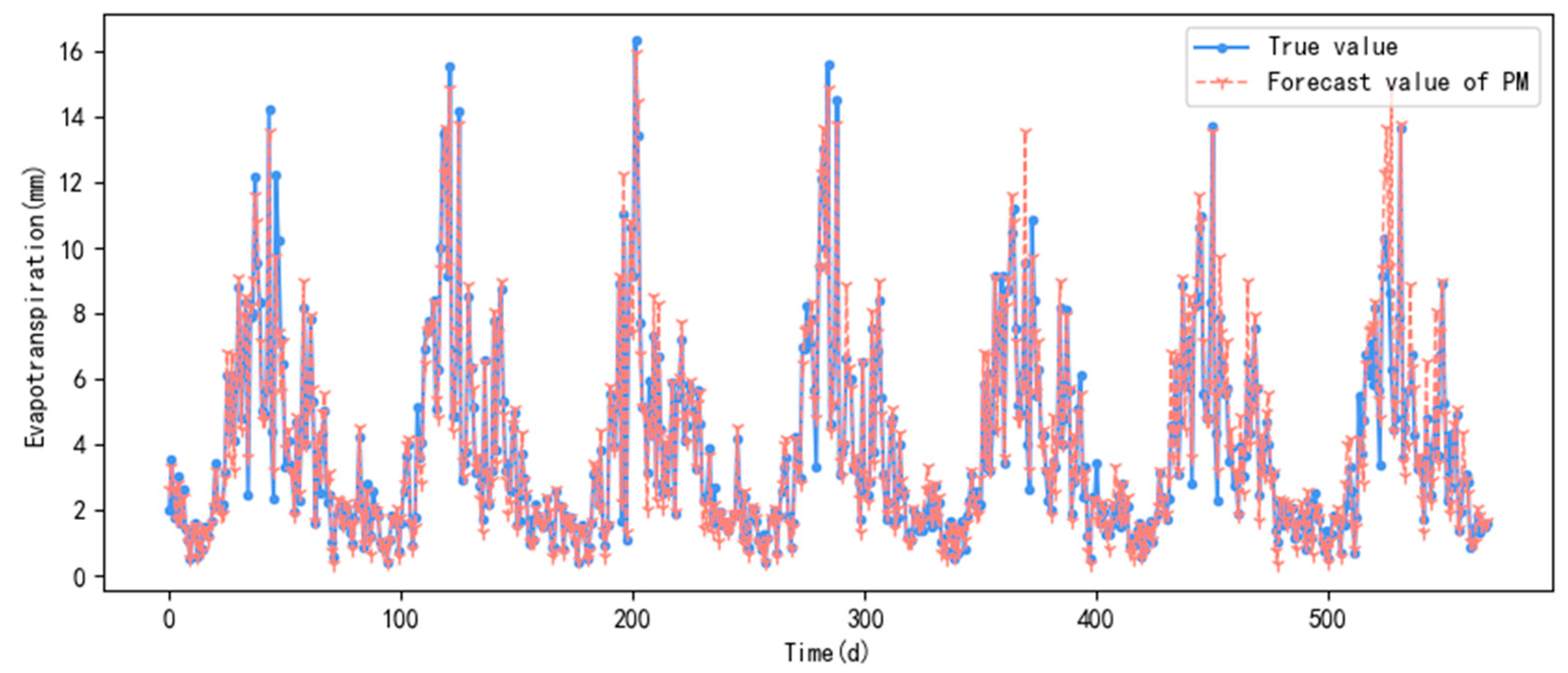
3.1. Forecast Reference Crop Evapotranspiration Based on Historical Meteorological Data
Aa direct method for predicting reference crop evapotranspiration based on historical meteorological data was implemented. First, historical meteorological data were used to calculate the reference crop evapotranspiration according to the FAO-PM formula mentioned in
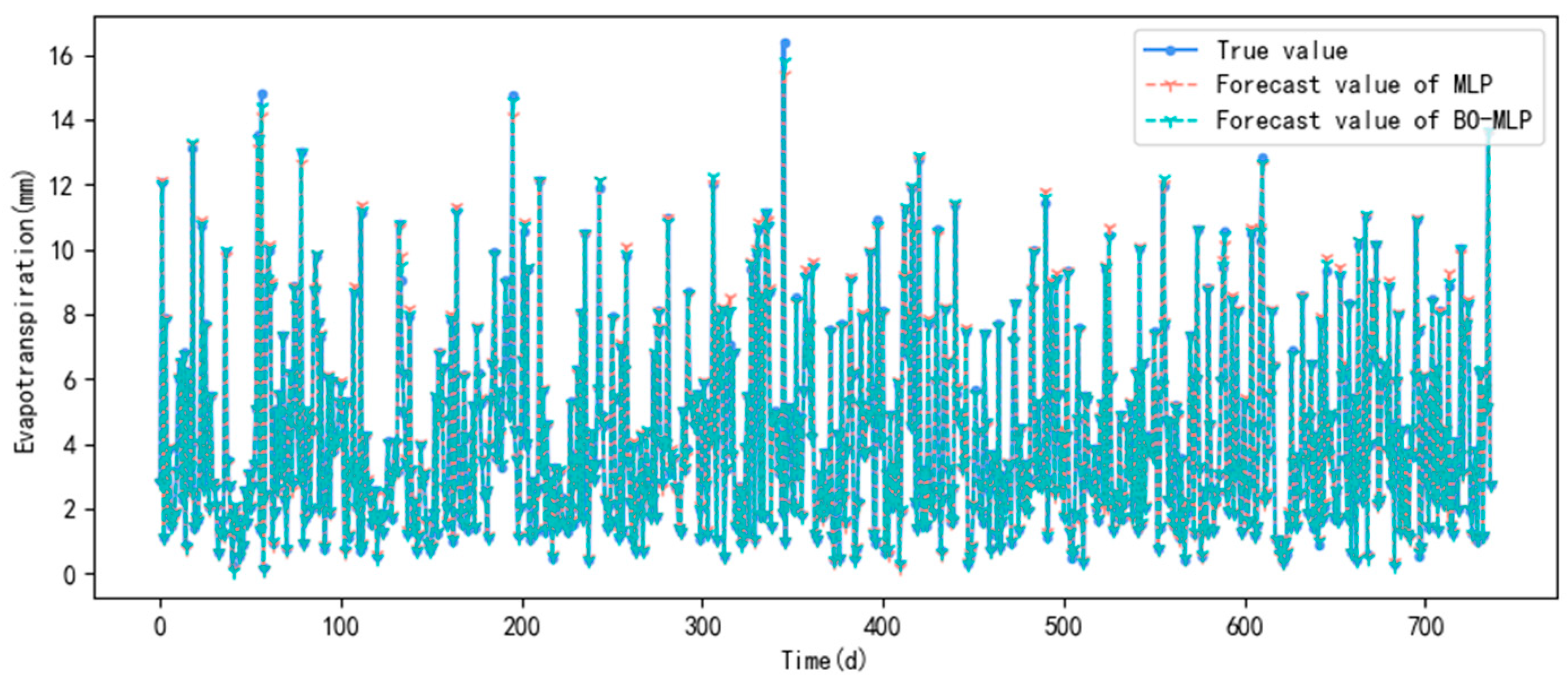
Section 2.2, and the result is then is used as the output of the machine learning model. Historical meteorological data were used as input to train reference crop evapotranspiration forecast model based on historical meteorological data. Finally, weather forecast data were used as input to test the forecast accuracy of the model.
The forecast results using MLP and BO-MLP on the historical meteorological data test set are shown in
Figure 1.
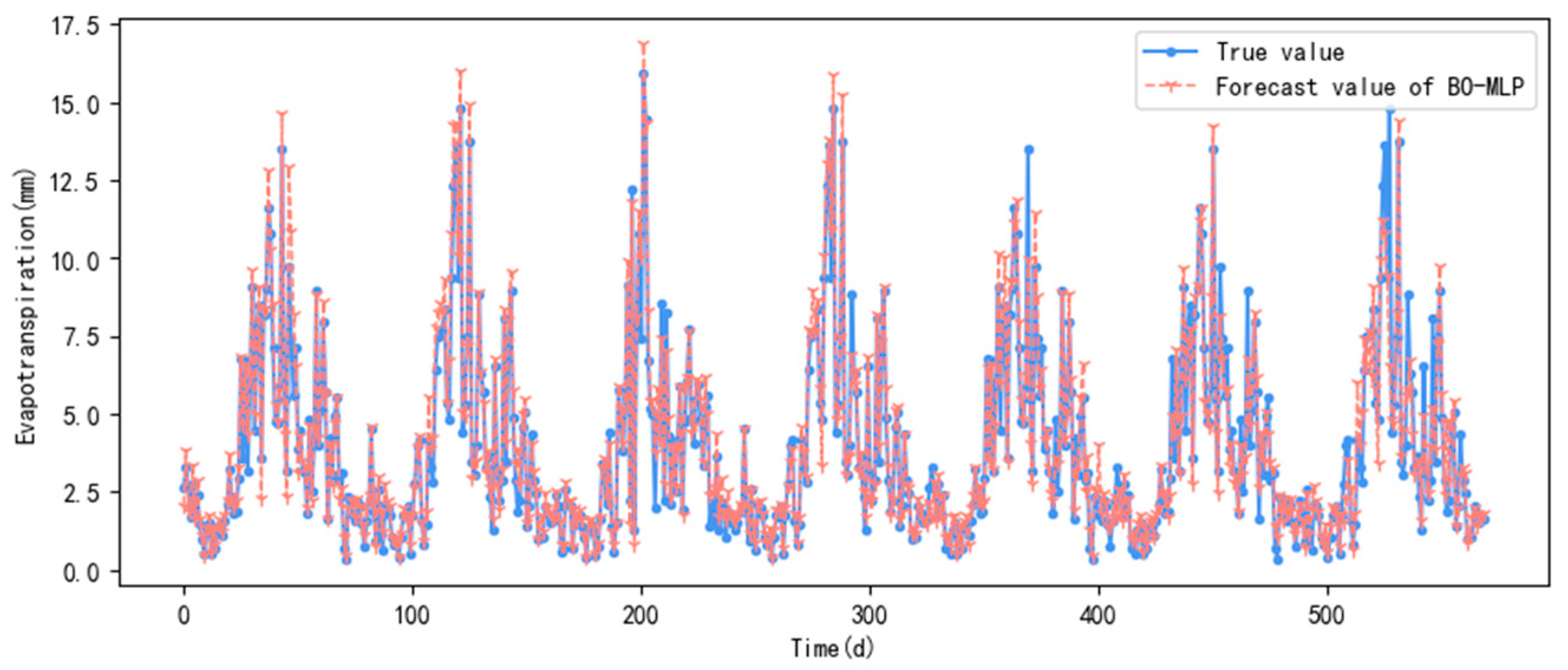
Because of the complete historical meteorological data, the prediction accuracy of MLP using the historical meteorological data test set is very high. Before tuning, RMSE, , and MAE were 0.12 mm/d, 0.9986, and 0.08, respectively. After tuning, the accuracy of the model was further improved, with RMSE as low as 0.07 mm/d, as high as 0.9996, and MAE of 0.04.
The forecast results using the BO-MLP model with the weather forecast dataset are shown in
Figure 2.
3.2. Forecast Reference Crop Evapotranspiration Based on Weather Forecast Data
In this section, the indirect method of forecasting reference crop evapotranspiration based on weather forecast data is considered. Weather forecast data were taken as input and historical meteorological data calculated by the PM formula were used as output to train the reference crop evapotranspiration model. Finally, the weather forecast test set was used to verify the model accuracy.
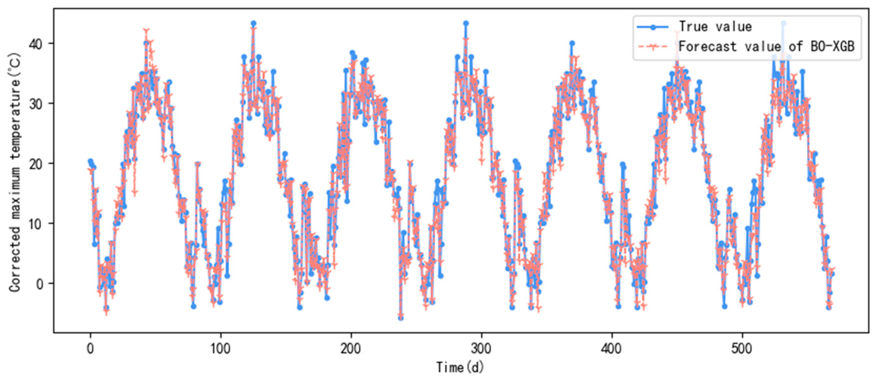
After path analysis and comparison of the above experiments, the BO-LGB model was used to construct the
forecast model based on weather forecasts using Combination 4 of meteorological factors as input. The forecast results using the test set are shown in
Figure 3.
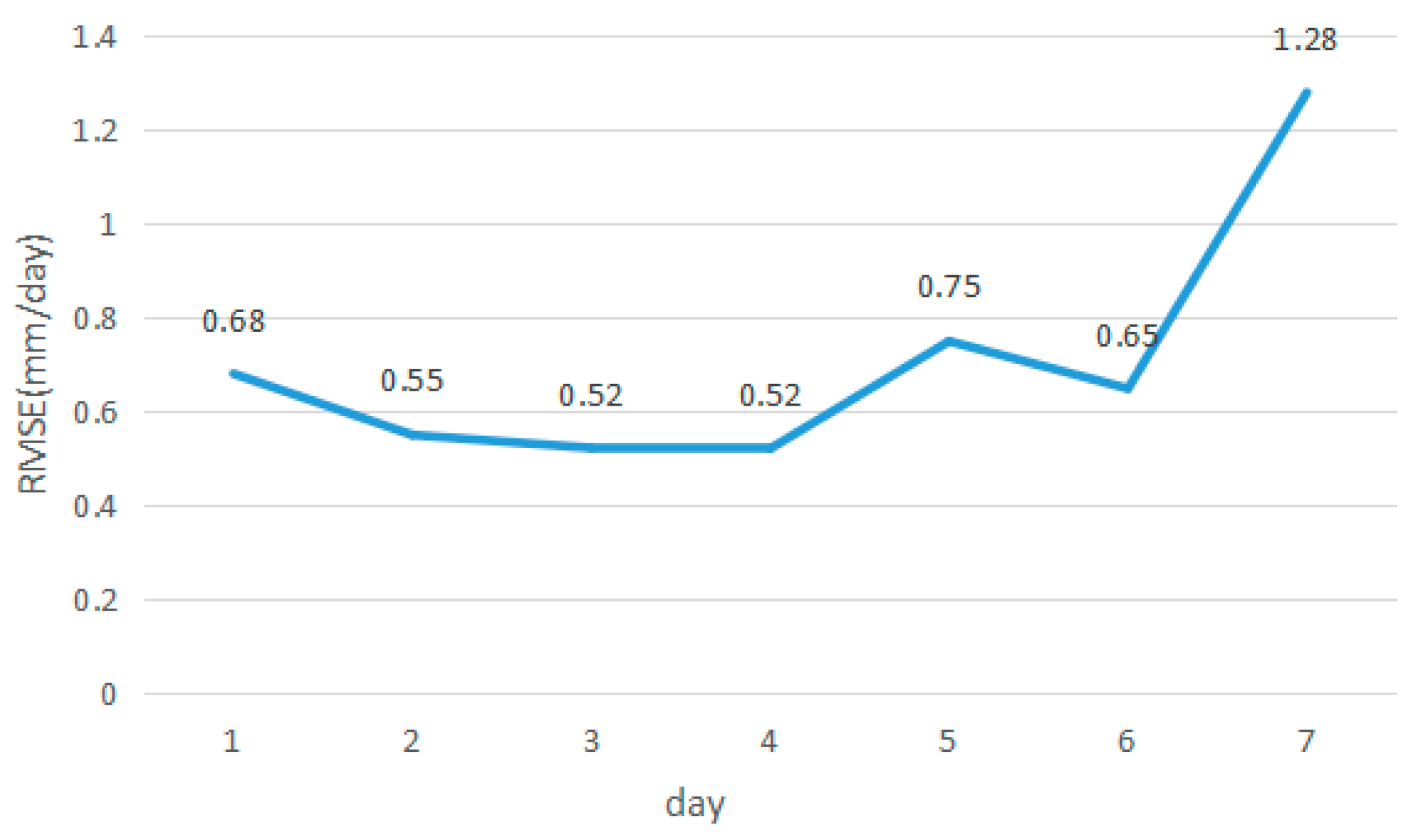
The RMSE values of the forecast results were calculated according to different forecast periods, as shown in
Figure 4.
The BO-LGB4 model based on weather forecast data was used to forecast . The value using the test set was 0.996, the MAE was 0.47, and the RMSE was 0.74 mm/day.
3.3. Forecast Reference Crop Evapotranspiration Based on Corrected Forecast Data
This section assesses weather forecast data as input and corresponding meteorological data in the historical meteorological data as output, using machine learning to complete the correction of weather forecast.
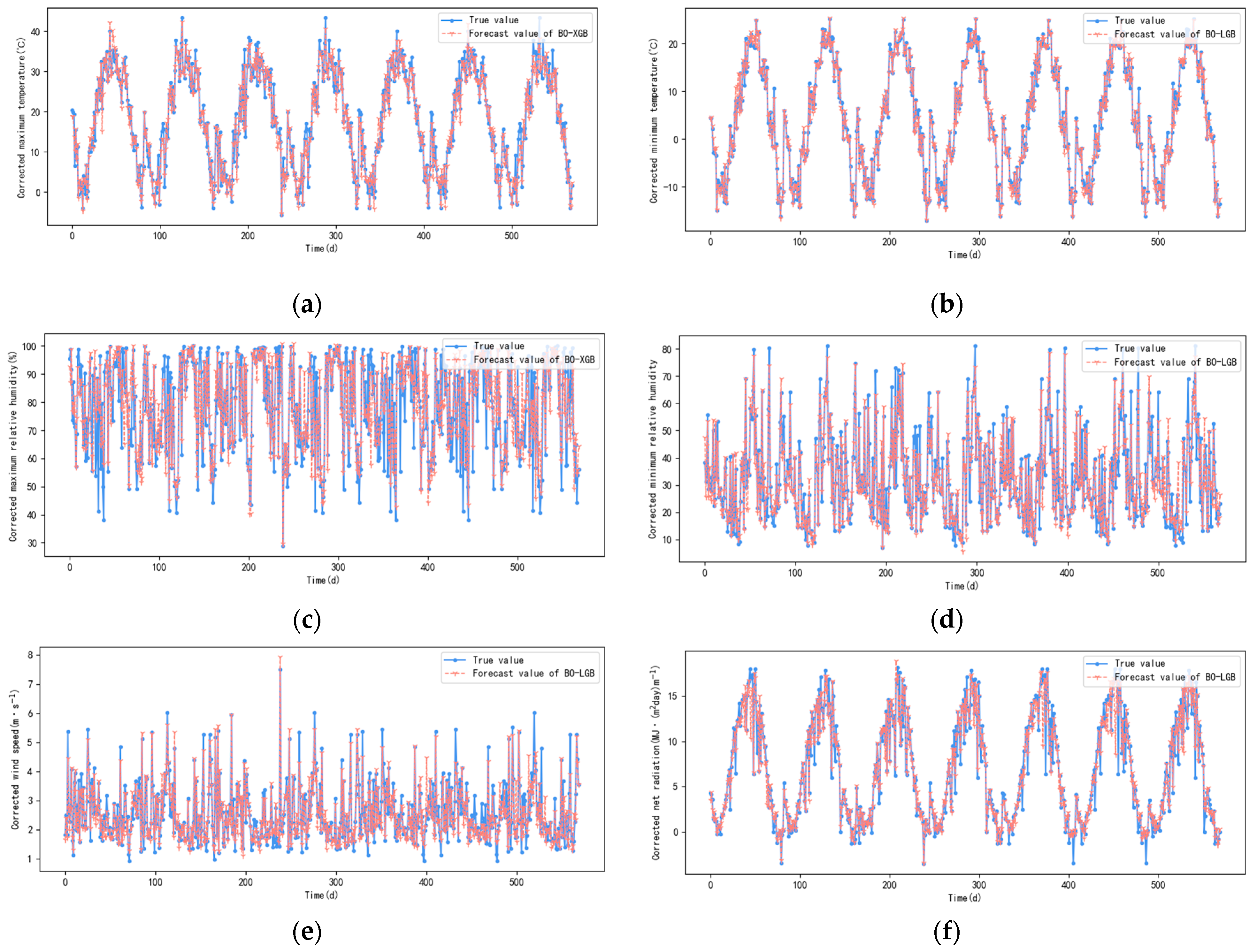
After the comparison of the above experiments, the weather Combination 2 selected via path analysis was finally used as the input, and the forecast factor correction model was constructed using BO-LGB and BO-XGB models. The forecast results using the test set were shown in
Figure 5.
For the test set, the RMSE for the correction of the maximum temperature was 1.49 °C, the RMSE for the correction of the minimum temperature was 1.03 °C, the RMSE for the correction of the maximum relative humidity was 6.63%, the RMSE for the correction of the minimum relative humidity was 5.38%, and the RMSE for the correction of the wind speed was 0.39 m/s. The RMSE of the corrected net radiation was 1.22 MJ/(m
2∙day). Using the corrected data and bringing it into the PM formula, the obtained prediction result of
is shown in
Figure 6.
was 0.93, MAE was 0.44 mm/day, and RMSE was 0.76 mm/day.
Using the corrected data, the BO-MLP model of
Section 2.4.2 was brought in, and the result of forecasting
is shown in
Figure 7.
was 0.93, MAE was 0.51 mm/day, and RMSE was 0.81 mm/day.
4. Discussion
First, the results of the three data sources were analyzed around parameters such as RMSE.
4.1. Forecast Model Based on Historical Meteorological Data
In the evaluation of model performance, historical weather data and corrected weather forecast data were used to compare the RMSE data size of the system. With the weather forecast dataset, the forecast accuracy of BO-MLP was greatly reduced, the forecast effect was not good, and the RMSE was 2.34 mm/d, which cannot meet practical application requirements. The reason for this analysis may be that the forecast accuracy is low and there is a prediction accuracy error, which makes the difference between the weather forecast data and the historical meteorological data large. Therefore, the weather forecast data cannot be used directly. So, it is necessary to correct the weather forecast data to obtain better accuracy and serve as the test data for the forecast model.
4.2. Forecast Model Based on Weather Forecast
The BO-LGB4 model based on weather forecast data was used to forecast . The value on the test set was 0.996, the MAE was 0.47, and the RMSE was 0.74 mm/day. The forecast accuracy was high, which met the application requirements. At the same time, the model was less affected by the forecast period. Except for the prediction period 7, the forecast accuracy significantly decreased, and the RMSE in other forecast periods was maintained between 0.520 and 0.748 mm/day.
4.3. Forecast Model Based on Corrected Weather Forecast
The BO-MLP model based on the corrected weather forecast data performed well for prediction. was 0.93, MAE was 0.51 mm/day, and RMSE was 0.81 mm/day. All of these reached the required accuracy range, but compared with the BO-LGB4 model based on weather forecast data, the level of optimization is not obvious. Since the weather forecast data must be corrected first before input, which increases the time consumption and computing power required, the authors believe that the use of corrected weather forecast data does not show enough advantage and practical value after consuming more computing power.
The authors think that the model based on weather forecast data has more application value.
Because changes in the weather are the result of the interaction of various factors, it is reasonable that the RMSE should increase with the increase of time. Moreover, due to the cumulative error in evapotranspiration forecasting, RMSE increases with time, but the error within seven days is still within the acceptable range, so the model can be defined as successfully established.
5. Conclusions
The purpose of this study is to propose a machine learning-based prediction model to serve precision irrigation scenarios and promote the application of DI. This paper attempts to compare the performance of historical meteorological data, weather forecasts, and corrected weather forecast data after processing by deep learning models such as MLP and random forest, and finally selects models and data sources that meet the accuracy expectations, exploring the possibility of applying machine learning methods in the field of precision agriculture. It provides a scientific basis for promoting agricultural water saving. Ultimately, the study created a forecast model based on weather forecast data that can predict irrigation demand over the next seven days with ideal accuracy.
5.1. Forecast Model Based on Historical Meteorological Data
Firstly, the path analysis between historical meteorological data and was carried out, and the conclusion drawn that the maximum temperature, radiation, and relative humidity have a great influence on , so the forecast accuracy of these meteorological parameters is related to the result accuracy of method 1. After model selection and Bayesian optimization, the forecast model based on historical meteorological data was obtained using MLP. The RMSE of the model on the historical meteorological data test set was 0.07 mm/day, and the RMSE on the weather forecast data set was 2.34 mm/day. The RMSE on the corrected weather forecast data test set was 0.81 mm/day. Due to the error of forecast accuracy in weather forecast and historical meteorological data, this method cannot be used between them, and better accuracy could be obtained only after the weather forecast was corrected.
The following are detailed descriptions of the three model processing steps:
5.2. Forecast Model Based on Weather Forecast
Firstly, path analysis was conducted on the weather forecast data and , and several meteorological factors with significant impact on were identified. These factors were combined into six different input combinations of meteorological factors. After model selection, it was determined that the model with J’, , , and as inputs had the highest accuracy. This indicates that path analysis can effectively identify input factors with a significant impact, thereby improving model accuracy and reducing overfitting. Through the comparison of random forest, LightGBM, and XGBoost models, it was found that the BO-LGB model had the highest accuracy, and the RMSE on the weather forecast test set was 0.74 mm/day.
5.3. Forecast Model Based on Corrected Weather Forecast
Firstly, path analysis was conducted between weather forecast data and corresponding historical meteorological data. This identified several meteorological factors that significantly impact the historical data, which were then divided into three input combinations. Combination 1 represents full factor correction, combination 2 involves multi-factor correction following path analysis selection, and combination 3 focuses on single-factor correction. Results reveal that combinations 1 and 2 exhibited higher accuracy compared with combination 3, with combination 2 showing lower overfitting than combination 1. Consequently, combination 2 was selected for weather forecasting factor correction. After comparing and optimizing the random forest, LightGBM, and XGBoost models, the corrected maximum temperature demonstrated an RMSE of 1.49 °C, the corrected minimum temperature had an RMSE of 1.03 °C, and the corrected maximum relative humidity exhibited an RMSE of 6.63%. The RMSE for minimum relative humidity correction was 5.38%, the RMSE for wind speed correction was 0.39 m/s, and the RMSE for net radiation correction was 1.22 MJ/(m2∙day). Incorporating the corrected weather forecast data into the PM formula, the RMSE for the forecast was 0.76 mm/day.
All three machine learning-based reference crop evapotranspiration prediction models achieved good accuracy, with the model based on weather forecast and the model based on corrected weather forecast demonstrating slightly higher accuracy, but with minimal difference. Considering the time cost, the direct use of weather forecast data is more suitable for practical applications. Analyzing the variation in model accuracy with the forecast period for the weather forecast-based forecast model reveals a general decrease in accuracy with longer forecast periods. However, the RMSE in the first six days showed little difference, ranging from 0.52 to 0.75 mm/day, while the prediction accuracy for the seventh day was slightly worse at 1.12 mm/day.
The limitation of this study is that the time span of the weather forecast data set was limited, the amount of data was small, and the accuracy of the model needs to be improved. Secondly, the time that can be predicted is relatively limited, and good accuracy can only be achieved for up to seven days. Finally, the prediction model has not been verified by experiments in actual scenarios.
Further attempts can be made to increase the time span, which should lead to stronger forecast accuracy, and then attempts to forecast a longer time horizon in the future to verify the accuracy. It is hoped that this experiment can be verified on a global scale to confirm the feasibility of the theory. It is also possible to try more deep learning models to optimize the speed of computation and improve the accuracy of computation.
Author Contributions
Conceptualization, J.L.; methodology, J.C.; software, J.C. and P.G.; validation, J.C. and P.G.; formal analysis, J.C.; investigation, J.C.; resources, J.L.; data curation, J.C.; writing—original draft preparation, P.G.; writing—review and editing, P.G.; visualization, P.G.; supervision, J.L.; project administration, J.L.; funding acquisition, J.L. All authors have read and agreed to the published version of the manuscript.
Funding
This research received no external funding.
Data Availability Statement
Data are contained within the article.
Conflicts of Interest
The authors declare no conflicts of interest.
References
- China Statistical Yearbook 2022. Available online: https://www.stats.gov.cn/sj/ndsj/2022/indexeh.htm (accessed on 5 February 2024).
- Ahmed, W.; Safdar, U.; Ali, A.; Haider, K.; Tahir, N.; Sajid, S.; Ahmad, M.; Khalid, M.; Sattar, M.T.; Khan, A.; et al. Sustainable Water Use in Agriculture: A Review of Worldwide Research. Int. J. Agric. Biosci. 2022, 11, 246–250. [Google Scholar] [CrossRef]
- Zhang, H.; Oweis, T. Water–Yield Relations and Optimal Irrigation Scheduling of Wheat in the Mediterranean Region. Agric. Water Manag. 1999, 38, 195–211. [Google Scholar] [CrossRef]
- Allen, R.G.; Pereira, L.S.; Raes, D.; Smith, M. Crop Evapotranspiration-Guidelines for Computing Crop Water Requirements-FAO Irrigation and Drainage Paper 56. FAO 1998, 300, D05109. [Google Scholar]
- Yin, J.; Deng, Z.; Ines, A.V.; Wu, J.; Rasu, E. Forecast of Short-Term Daily Reference Evapotranspiration under Limited Meteorological Variables Using a Hybrid Bi-Directional Long Short-Term Memory Model (Bi-LSTM). Agric. Water Manag. 2020, 242, 106386. [Google Scholar] [CrossRef]
- de Oliveira e Lucas, P.; Alves, M.A.; e Silva, P.C.D.L.; Guimaraes, F.G. Reference Evapotranspiration Time Series Forecasting with Ensemble of Convolutional Neural Networks. Comput. Electron. Agric. 2020, 177, 105700. [Google Scholar] [CrossRef]
- Ensemble Methods for Neural Network-Based Weather Forecasts—ProQuest. Available online: http://www-proquest-com-s.vpn1.bjfu.edu.cn:8118/docview/2492673684?pq-origsite=wos&accountid=42626&sourcetype=Scholarly%20Journals (accessed on 20 March 2024).
- Hargreaves, G.H.; Samani, Z.A. Reference Crop Evapotranspiration from Temperature. Appl. Eng. Agric. 1985, 1, 96–99. [Google Scholar] [CrossRef]
- Priestley, C.H.B.; Taylor, R.J. On the Assessment of Surface Heat Flux and Evaporation Using Large-Scale Parameters. Mon. Weather. Rev. 1972, 100, 81–92. [Google Scholar] [CrossRef]
- Wright, S. Correlation and Causation. J. Agric. Res. 1921, 20, 557–585. [Google Scholar]
- Barth, E.; de Resende, J.T.V.; Mariguele, K.H.; de Resende, M.D.V.; da Silva, A.L.B.R.; Ru, S. Multivariate Analysis Methods Improve the Selection of Strawberry Genotypes with Low Cold Requirement. Sci. Rep. 2022, 12, 11458. [Google Scholar] [CrossRef] [PubMed]
- Shaheen, M.; Abdul Rauf, H.; Taj, M.A.; Yousaf Ali, M.; Bashir, M.A.; Atta, S.; Farooq, H.; Alajmi, R.A.; Hashem, M.; Alamri, S. Path Analysis Based on Genetic Association of Yield Components and Insects Pest in Upland Cotton Varieties. PLoS ONE 2021, 16, e0260971. [Google Scholar] [CrossRef] [PubMed]
- Yuan, Z.F.; Zhou, J.Y.; Guo, M.C.; Lei, X.Q.; Xie, X.L. Decision Coefficient-the Decision Index of Path Analysis. J. Northwest Sci-Tech Univ. Agric. For. 2001, 29, 131–133. [Google Scholar]
- Jamshidi, S.; Zand-parsa, S.; Pakparvar, M.; Niyogi, D. Evaluation of Evapotranspiration over a Semiarid Region Using Multiresolution Data Sources. J. Hydrometeorol. 2019, 20, 947–964. [Google Scholar] [CrossRef]
- Kumar, V.; Garg, M.L. Deep Learning Techniques and Their Applications: A Short Review. Biosci. Biotech. Res. Comm. 2018, 11, 699–709. [Google Scholar] [CrossRef]
- Breiman, L. Random Forests. Mach. Learn. 2001, 45, 5–32. [Google Scholar] [CrossRef]
- Morgan, J.N.; Sonquist, J.A. Problems in the Analysis of Survey Data, and a Proposal. J. Am. Stat. Assoc. 1963, 58, 415–434. [Google Scholar] [CrossRef]
- Davis, R.A.; Nielsen, M.S. Modeling of Time Series Using Random Forests: Theoretical Developments. Electron. J. Stat. 2020, 14, 3644–3671. [Google Scholar] [CrossRef]
- Govorov, M.; Beconytė, G.; Gienko, G.; Putrenko, V. Spatially Constrained Regionalization with Multilayer Perceptron. Trans. GIS 2019, 23, 1048–1077. [Google Scholar] [CrossRef]
- Chen, T.; Guestrin, C. XGBoost: A Scalable Tree Boosting System. In Proceedings of the 22nd ACM SIGKDD International Conference on Knowledge Discovery and Data Mining, San Francisco, CA, USA, 13–17 August 2016; ACM: New York, NY, USA, 2016; pp. 785–794. [Google Scholar]
- Suhartono, D.; Gema, A.P.; Winton, S.; David, T.; Fanany, M.I.; Arymurthy, A.M. Hierarchical Attention Network with XGBoost for Recognizing Insufficiently Supported Argument. In Multi-Disciplinary Trends in Artificial Intelligence; Phon-Amnuaisuk, S., Ang, S.-P., Lee, S.-Y., Eds.; Lecture Notes in Computer Science; Springer International Publishing: Cham, Swizterland, 2017; Volume 10607, pp. 174–188. ISBN 978-3-319-69455-9. [Google Scholar]
- Ke, G.; Meng, Q.; Finley, T.; Wang, T.; Chen, W.; Ma, W.; Ye, Q.; Liu, T.-Y. Lightgbm: A Highly Efficient Gradient Boosting Decision Tree. In Proceedings of the 31st Conference on Neural Information Processing Systems (NIPS 2017), Long Beach, CA, USA, 4–9 December 2017. [Google Scholar]
- Zhang, J.; Mucs, D.; Norinder, U.; Svensson, F. LightGBM: An Effective and Scalable Algorithm for Prediction of Chemical Toxicity–Application to the Tox21 and Mutagenicity Data Sets. J. Chem. Inf. Model. 2019, 59, 4150–4158. [Google Scholar] [CrossRef] [PubMed]
- Akhavizadegan, F.; Ansarifar, J.; Wang, L.; Huber, I.; Archontoulis, S.V. A Time-Dependent Parameter Estimation Framework for Crop Modeling. Sci. Rep. 2021, 11, 11437. [Google Scholar] [CrossRef]
| Disclaimer/Publisher’s Note: The statements, opinions and data contained in all publications are solely those of the individual author(s) and contributor(s) and not of MDPI and/or the editor(s). MDPI and/or the editor(s) disclaim responsibility for any injury to people or property resulting from any ideas, methods, instructions or products referred to in the content. |
© 2024 by the authors. Licensee MDPI, Basel, Switzerland. This article is an open access article distributed under the terms and conditions of the Creative Commons Attribution (CC BY) license (https://creativecommons.org/licenses/by/4.0/).


