Abstract
One of the challenges in site-specific phosphorus (P) management is the substantial spatial variability in plant available P across fields. To overcome this barrier, emerging sensing, data fusion, and spatial predictive modeling approaches are needed to accurately reveal the spatial heterogeneity of P. Seven spatially variable fields located in Ontario, Canada are clustered into two zones; four fields are located in eastern Ontario and three others are located in western Ontario. This study compares Bayesian Additive Regression Trees (BART), Support Vector Machine regressor (SVM), and Ordinary Kriging (OK), along with novel data fusion concepts, to analyze integrated high-density spatial data layers related to spatial variability in soil available P. Feature selection and interaction detection using BART variable selection and Recursive Feature Elimination (RFE) for SVM were applied to 42 predictors, including soil-vegetation indices derived from PlanetScope multispectral imagery, high-density apparent soil electrical conductivity (ECa), and high-resolution topographic attributes derived from DUALEM-21S and a Real-Time Kinematic (RTK) global navigation satellite systems (GNSS) receiver, respectively. Modeling spatial heterogeneity of soil available P with BART showed higher accuracy than SVM and OK in both zones of this study when trained and tested on ground truth data from clusters of farms. A BART variable selection approach resulted in six auxiliary predictors of soil available P in the eastern zone, while only four predictors were selected to predict P in the western zone. RFE for SVM resulted in models with 15 and 12 auxiliary predictors in the eastern and western Ontario zones. Topographic elevation was the most influential predictor of soil available P in both zones. Compared with the SVM and OK methods, BART exhibited lower average RMSE values for individual fields of 1.86 ppm and 3.58 ppm across the eastern and western Ontario zones, respectively, along with higher R2 values of 0.85 and 0.83, respectively. In contrast, SVM had RMSE values for individual fields in the eastern and western Ontario zones, respectively, averaging 5.04 ppm and 7.51 ppm and R2 values of 0.27 and 0.43. RMSE values for soil available P in individual fields across the eastern and western Ontario zones averaged 4.77 ppm and 7.81 ppm, respectively, with the OK method, while R2 values averaged 0.19 and 0.44. The selection of suitable auxiliary predictors and data fusion, combined with BART spatial machine learning algorithms, have potential to be a useful tool to accurately estimate spatial patterns in soil available P for agricultural fields in Ontario, Canada.
1. Introduction
Phosphorus (P) is an essential nutrient for plants. P is involved in many fundamental biological processes such as photosynthesis, cell division, and enlargement. Root expansion and length and seed formation depend mainly on P uptake by the plant. P is a non-renewable resource and cannot be replaced by any other element [1]. Therefore, it is important to conserve these finite resources to fertilize soils and feed future generations.
A world population expected to reach 9.1 billion by 2050 requires a rise in food production of 70% [2]. However, soil is becoming degraded in many parts of the world, meaning that agriculture can only occur in a limited area. Thus, it is essential that this limited area be accompanied by an increase in soil productivity with respect to sustainable development and environmental protection. If soils at agricultural sites are deficient in P, it can lead to up to 15% yield losses [3]. To overcome this issue, farmers will often add P fertilizers to adjust soil fertility and maximize yields. Similarly, yield can be improved in field zones where fertilizer application is needed, while reducing over-fertilization in zones that have limited yield potential [4]. Implementing this precision agriculture approach requires data collection, preprocessing and analysis, and spatial variability modeling, as well as technological advances in remote and proximal sensing [5].
When applying P fertilizer on fields, farmers will typically apply a uniform P rate. However, soil P spatial variability in field scale tends to be high in most places [6]. Thus, applying a uniform P rate neglects P spatial variation within soils and can lead to over or under application of fertilizers. This increases production input costs, and excess P may runoff into surrounding ecosystems [7]. One solution to this issue is to adopt precision agriculture, which involves dividing fields into zones and delivering customized management to each zone [8]. The concept behind precision agriculture is based mainly on the use and combination of different sources of digital information to respond to field variability, while enhancing profitability and preserving ecological and agroecosystem quality. Hence, due to natural variability in the field, site-specific management strategies provide promising results in terms of profitability, product quality, and rational use of inputs. Using technology and precision farming tools, farmers can avoid applying uniform input rates for the whole parcel and thereby manage soil sustainably. The goal of precision nutrient management is to ensure that each zone in the field receives a rate of fertilizer that is specific to that zone’s requirement [9,10].
Because spatial variability is usually high for most soil properties, high-resolution soil property maps can help farmers identify in-field variability in soil, assess soil and crop health, and boost soil productivity by relying on precision fertilization management. However, precision P fertilization management is still not considered in most arable land. Increasing phosphorus fertilizer prices and concerns over the efficient use of a limited resource has increased the need for innovative spatial prediction methods in agricultural fields to optimize the use of P fertilizer. We hypothesize that the integration and fusion of different sources of digital data and the application of machine learning-based predictive models will help farmers obtain more accurate estimates of soil P spatial variability and improve their ability to develop variable rate P prescriptions.
Data availability and collection represent major concerns of the past two decades, with an aim to boost soil productivity, take rational management decisions, and reduce P losses in runoff. The development of proximal sensor technology is making a great difference by allowing the collection of voluminous and diverse data to farm practitioners and agricultural policy experts [11]. However, no commercial sensor exists for on-the-go available phosphorus measurements. Various research sensor and soil reflectance techniques offer promise towards attaining this goal [12]. The integration and fusion of different proximal soil sensors could provide farmers with robust soil P predictions, rather than relying on the use of a single sensor to predict spatial patterns in P [13]. Data integration plays a key role in producing effective machine learning models by incorporating data from a variety of sources [14]. Therefore, the fusion of suitable sensor data in the process of variable rate management decisions should be tested to determine whether it would improve farmer’s profitability and reduce environmental impacts.
Soil property mapping has mostly depended on traditional soil surveys, which requires substantial costs and time for soil sample collection and laboratory analysis. This approach is ineffective and time consuming, and often does not specifically capture the spatial variability present in soil P due to its focus on soil pedological characteristics at coarse sampling density and resolution [15,16]. Alternatively, technological advances in earth observation technologies have made the digital soil mapping of important soil properties economically feasible for the soil community. Remote sensing constellations provide a wide range of data quality, quantity, and spatial coverage to gather information about the earth surface and atmosphere at different scales [17]. Particularly, the recent emerging microsatellite constellations of PlanetScope offer global high spatial resolution images of red–green–blue (RGB) and near infrared (NIR) bands at 3 to 5 m spatial resolution. In general, the mixed effect in raster cells is minimized by using higher spatial resolution products, which leads to more pure soil pixels for model development [18]. Hence, higher spatial resolutions of multispectral images could provide accurate spectral signatures of bare soils to spatially predict soil available P. These remote sensing auxiliary data have been used for agricultural [19] and environmental monitoring [20], land use mapping [21], soil salinity [22], crop type and land cover mapping [23], daily monitoring of crop Leaf Area Index (LAI) [24], clay, sand, organic matter, iron contents, and soil color [25], and soil organic carbon mapping [26].
Various spatial prediction approaches have been used to assess the spatial variability of soil properties. In fact, multiple linear regression and Kriging are two of the most used approaches, probably because they are easy to produce and interpret. Regression Kriging, which combines covariates correlation and spatial autocorrelation, provides better estimates of soil properties by reducing prediction errors [27,28,29,30]. However, Regression Kriging performance depends on the relationship between the soil property of interest and the environmental predictors. This makes the algorithm unstable across many case studies [31]. Furthermore, geostatistical approaches applied to digital soil mapping in general have several limitations. First, residuals are assumed normally distributed, stationary, and isotropic. Second, geostatistics in digital soil mapping fails to handle the non-linear relationship between high-dimensional and/or correlated covariates and the target soil property. In addition, geostatistical models are not able to capture steady and sudden changes in soil variability with semivariograms [32,33]. Alternatively, ML algorithms have shown promising improvements in accuracy of predicting SOM and other soil properties relative to simpler linear regression approaches, Ordinary Kriging and Regression Kriging [34].
Predictive modeling of soil properties can be obtained by fitting multiple linear regression models to infer the relationship between environmental predictors and the soil property of interest. However, this relationship is often non-linear in nature. That is why, for example, a very low predictive performance was reported when using traditional linear regression models to predict NPK nutrients using PlanetScope imagery [35]. Conversely, advances in computing performances and algorithms, data storage, and high-resolution multispectral images have led to an improvement in the digital soil mapping of soil properties. To overcome this issue of non-linearity and the complexity of multidimensional feature spaces, machine learning models were designed to capture the non-linear relationship between the dependent auxiliary variables and the target variable. For example, machine learning and data mining algorithms have been applied to a wide range of questions relating to the spatial predictions of soil classes and continuous soil properties. Statistical learning methods have been used to assess soil fertility and available nutrients such as nitrogen, cation exchange capacity, and soil organic carbon [36,37], as well as phosphorus and potassium [38,39]. On the other hand, categorical soil properties such as soil taxonomic units [40] and soil texture class [41] have been generated using ML algorithms.
Georeferenced fused datasets, involving the integration of a suitable soil sampling design and a selection of powerful environmental predictors, could be used in the training and validation of predictive spatial models of important soil properties. Machine learning algorithms have been utilized in the spatial prediction of soil properties, but we are not aware of the previous integration and fusion of high-density proximal soil sensor data with remote sensing-derived indices for soil available P spatial modeling. Previous studies have used PlanetScope imagery along with other remote sensing products such as the Landsat and Sentinel series of satellites to extract more information from reflectance bands in the shortwave and red edge portion of the electromagnetic spectrum. On the other hand, few studies account for the accuracy assessment of predicted maps in digital soil mapping [32]. Previous studies have generally focused on the predictions of soil properties at regional [42,43,44,45,46] or within a single field scale [47,48] rather than heterogeneous clustered fields.
The overall goal of this study is to examine how the integration and fusion of different data sources can be used to increase the accuracy in soil available P spatial predictions for seven different spatially clustered fields across Ontario, Canada using machine learning algorithms. A key objective of this research study is to evaluate the prediction performance of two machine learning algorithms, including Bayesian Additive Regression Trees (BART machine) and Support Vector Machine (SVM), and attempt to tune their hyperparameters to achieve a balance between prediction accuracy and calibrated uncertainty intervals in the cross-validation process. In this study, we use SVM as a supervised machine learning algorithm and BART as an ensemble method that uses the Bayes theorem. These machine learning methods are compared with the Ordinary Kriging (OK) geostatistical approach, which is widely used in soil P mapping. SVM and OK are popular in predictive soil mapping, but BART has not previously been applied to the spatial prediction of soil fertility variable such as P. BART is an advanced adaptation of the random forest method, which has already been used to study soil fertility variables [49]. We also aim to investigate the importance of different types of auxiliary predictors in predicting soil available P to understand how they can contribute to generating robust spatial predictions that can help guide soil P modeling and P precision fertilization management. In other words, we attempt to evaluate how much gain in prediction performances can be attributed to each auxiliary data variable. One therefore must ask: can soil available P be easily related to auxiliary variables? We ask this question because even though machine learning models provide accurate results, interpretability and causality are still challenging for the soil scientific community [50].
2. Materials and Methods
The flow chart in Figure 1 represents a summary of the workflow adopted in this research project to design and select spatial predictive models for soil available P. All data processing and statistical analysis were carried out using the R statistical software version 4.2.0 (R development Core Team, 2022). The workflow steps are described in detail below.
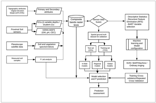
Figure 1.
Schematic illustrating the workflow for machine learning model development and spatial predictive modeling of soil available P within the study sites of this research project.
2.1. Study Area
Soil sampling and proximal soil sensing occurred in seven spatially distributed fields located in western or eastern Ontario, Canada. Soil samples and proximal soil sensor (PSS) data were collected by the department of bioresource engineering team at McGill University [49]. Figure 2 illustrates the field locations, boundaries, and soil sampling locations. Data from this study were collected and processed in the NAD83 datum (North American Datum)/UTM (Universal Transverse Mercator) projection system. Four fields of this study are in the eastern Ontario (UTM 18N) zone near Greely, and three others are in the western Ontario (UTM 17N) zone near Guelph. Guelph field cluster (UTM 17N zone) is mostly Gray–Brown Luvisols, which have calcareous parent material. The Greely field cluster (UTM 18N zone) is mostly Melanic Brunisols, which tend to be acidic. Guelph soil texture is mainly loam to silt loam, and Greely soil texture is ranging from clay to silt loam [51].
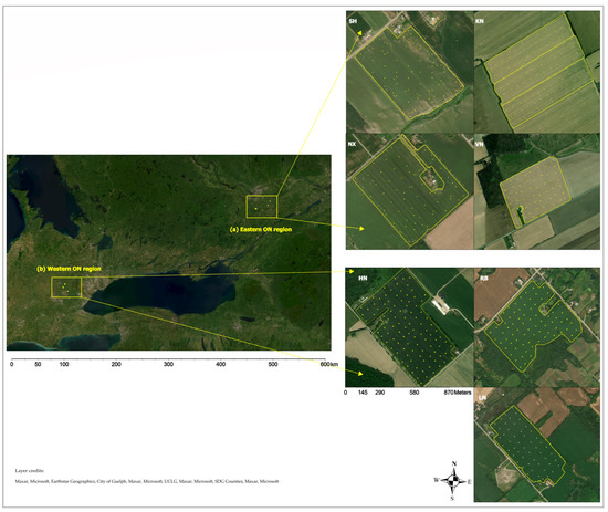
Figure 2.
Seven fields representing the study area in Ontario, Canada. Dots illustrate the locations of soil samples in two clusters of fields located in Greeley, eastern Ontario cluster of four fields (UTM 18N): NX (44.47 ha), SH (49.80 ha), VN (20.43 ha), KN (48.14 ha) fields, and Guelph, western Ontario cluster of three fields (UTM 17N): LN (21.14 ha), RB (30.32 ha), HN (39.37 ha). The total area covered by this research project is about 244 ha, at an average sampling density of two cores per hectare. Ground truth soil samples are fused and integrated with environmental predictors to develop ML spatial models for soil available P.
2.2. Data Collection and Preprocessing
2.2.1. Spatial Coverage of Soil Sampling
Soil samples were collected based on a regular grid (field ID codes KN, VN, HN, RB, LN) or a combination of random and directed (NX, SH) sampling. In total, 479 composite samples were collected along with GPS locations. Composite samples are made of up to 10 core samples with an approximate depth of 15 cm. The physical soil sampling density is roughly two samples per hectare. The maximum distance between a pair of points is estimated at 672 m, while the minimum is 64 m. Soil samples were collected and analyzed as ground truth data for the spatial modeling of soil available P. Laboratory measured extractable phosphorus (P) was carried out using the P—Olsen sodium bicarbonate test method. Measurements of soil available P are expressed in ppm. Supplementary Table S1 summarizes more details related to the number of soil samples per field, available PSS covariates, number of PSS readings per field for each PSS sensor, and acronyms for predictive models based on the geographic UTM zone where fields are located.
2.2.2. Proximal Soil Sensing
Two proximal soil sensors were used to map these fields. Sensors were mounted on an all-terrain vehicle (ATV) at about 60 cm above the soil surface to record readings on parallel lines at about 12 m apart from each other. Sensor readings were recorded every second and the travel speed was estimated at 10 km/h.
ECa Measurements
Apparent Electrical Conductivity (ECa) readings were collected using an electromagnetic induction instrument (DUALEM-21s, Milton, ON, Canada). This sensor is equipped with two pairs of electromagnetic receivers: horizontal coplanar geometry—HCP and perpendicular geometry—PRP. Sensor readings were obtained from four different depths: HCP1—0–1.6 m (ECa0–1.6), PRP1—0–0.5 m (ECa0–0.5), HCP2—0–3.2 m (ECa0–3.2), and PRP2—0–1 m (ECa0–1.0).
Topographic Attributes
Trimble AgGPS 542 GNSS receiver and base station (Trimble, Inc., Sunnyvale, CA, USA) were used to derive accurate and high-density elevation data. High-density elevation data were collected at all study sites at about 3000 points/ha (Supplementary Table S1). ArcGIS Pro 3.0.3 software was used [52] to produce digital elevation models (DEMs) and derive primary and secondary topographic attributes at 3m spatial resolution (Table 1).

Table 1.
Primary and secondary topographic attributes considered in this research project.
2.2.3. Remote Sensing Data Acquisition and Preprocessing
PlanetScope remote sensing products were selected in this study as a source of explanatory variables due to their high spatial resolution and short revisit time. PlanetScope consists of a constellation of approximately 130 cube-satellites orbiting the earth. This sensor provides up to 3 m per pixel spatial resolution in the visible (Red, Green, and Blue) and near-infrared (NIR) reflectance bands (i.e., PSSscene4Band type). These data are available for download via Planet’s APIs at https://www.planet.com/explorer/, accessed on 31 January 2024. PlaneScope Ortho Analytic 4B SR level 3B satellite imagery were acquired in a ready-to-use format. This surface reflectance 4-band image product is suitable for analytical applications, as it has scene-based framing and cartographic projection. Images are orthorectified to remove terrain distortions and radiometrically corrected based on specific atmospheric conditions and location-specific spectral response. Ortho tiles were mosaicked and cropped to cover the extent of our study sites. Cloud cover was set to be less than 5% in case raster images with 0.00% cloud cover were not available [58,59].
Datasets generated by this sensor suit our needs to assess the spectral signature of bare soils. We downloaded and processed high spatial resolution PlanetScope multispectral images from bare fields. To filter results of the Planet explorer and get the best available bare soil imagery, we specified not only a range of data collection days and imagery type, but also environmental conditions to minimize cloud cover, haze, and snow. Dates of fall imagery were 18–19 October 2017 in western Ontario and 28 October 2017 in eastern Ontario. Dates of spring imagery in western and eastern Ontario were 14 May 2017, and 24 April, and 12 May 2017, respectively. In North America, soils are bare following the harvest of primary crops in late September to late November, and after snowmelt in mid-April to mid-May. Therefore, two layers of PlanetScope-derived soil and vegetation indices were produced for the same index, one in fall and one in spring. The list of indices used for spatial modeling of available P are detailed in Table 2. These raster layers were prepared using ArcGIS Pro 3.0.3 software [52].
Table 2.
PlanetScope bands, soil and vegetation indices considered in this research project.
2.3. Sensor Data Fusion
The fused dataset consists of a spatial matrix of measured soil observations and corresponding values of available predictors. This spatial matrix was built as input to Support Vector Machine (SVM) and Bayesian Additive Regression Trees (BART) machine learning algorithms. We used the raster to points function in ArcGIS Pro [52] to collect values of PSS and RS predictors at locations (X and Y) of measured soil P. This allowed us to proceed to sensor data fusion and integrate all collected data in space. The fused spatial dataset was then considered as the ground truth dataset, which we used during the training and validation of our machine learning spatial prediction models (see Section 2.4 about machine learning and model configurations). Powerful predictors were then identified by each machine learning model (see Section 2.6 and Section 3.3 for more details about variable selection approaches).
2.4. Machine Learning and Model Configurations
P is considered as our target variable in the fused sensor and soil-laboratory datasets. P was considered as a continuous target variable while dealing with spatial regression modeling. BART machine and SVM machine learning models were compared with the Ordinary Kriging (OK) interpolation method, to test how these models can learn from the spatially fused dataset to make P spatial predictions with an acceptable accuracy.
Models for this study were developed starting with the available auxiliary PSS data for each of the individual seven fields. Fields of this study are located in two distinct regions. Therefore, we developed separate ML spatial models for each field and then for each region (i.e., western and eastern Ontario regions) using PlanetScope RS indices, topographic attributes, Dualem-21S data, and the training observations for soil P. A third approach to building valid predictive models for P is to use the overall global spatial point observations from all seven. Regression results for models produced in each zone and the “global” model are compared and evaluated.
2.4.1. Data Preprocessing
The fused dataset was centered and scaled before building our spatial predictive machine learning models. Centering and scaling were applied to predictors before running SVM machine learning models. Centering the data refers to mean subtraction from each observation in the fused dataset. Scaling consists of dividing independent predictors by their standard deviation. No data transformation for the BART algorithm was required, which has automated built-in functions for the centering and scaling of predictors. These preprocessing techniques were applied to transform all covariates on the same comparable scale which should improve our algorithm performances. All steps were seeded so the results are reproducible.
2.4.2. Algorithm Configuration, Model Fitting and Validation
Model fitting and validation was achieved using the ‘caret’ package [68,69] in the statistical program R [70]. We tuned each model hyperparameters and specified respective and specific arguments for each model. Caret also includes the “tunelength” argument of the “train()” function which helps in hyperparameter estimation. The “train()” function in ‘caret’ package was used to run SVM, while the BartMachine package was used to run the BART algorithm [71].
The process of evaluating the performance of machine learning models on unseen data is considered as a crucial step to determine how well models will generalize to new cases. This modeling process step helps to prevent overfitting, which occurs when a model is too closely fit to the training data and performs poorly on new data. It is important to perform model assessment and validation to ensure that the model is not overfitting the training data and to have a good estimate of its performance on new data.
In this study, we divided the fused dataset observations into training (75%) and testing (25%) sets. Models are trained on the training set and validated on the testing set. This provides an estimate of the model’s performance on new data. The training set is shuffled using repeated cross-validation, train, and control techniques. This allowed us to tune hyperparameters and, consequently, test and contrast different predictive models. Models were tested (calibrated) on unseen data partitions produced during each resampling iteration. To test the accuracy of our models on unseen data, we used a repeated cross validation resampling technique (test option) to improve our regressor model products. This test option is effective when the sample size is relatively small. Repeated cross-validation techniques were used to split the data into k-folds of equal size, and the model is trained on k-1 folds and evaluated on the remaining fold. Resampling of the spatial dataset process is repeated n times, each time with a different fold from the evaluation set. Consequently, the “caret” package runs n models and the average performance across all folds is used as an estimate of the model’s performance. Large n iterations are recommended to avoid overlap among test observations from different iterations [68]. In our case, we used 10-fold repeated cross validation with 100 iterations as a resampling approach for our spatial dataset which resulted in 1000 different subsets for model testing. The “Traincontrol” function in the “caret” package was used while training and testing our models.
The resampling approach builds and trains models based only on a portion of the sampled locations (i.e., training set). The “out-of-bag” or hidden dataset (i.e., testing set) is used for model validation and for computing performance metrics.
2.5. Machine Learning and Geostatistical Modeling Methods
2.5.1. Bayesian Additive Regression Trees
Bayesian Additive Regression Trees (BART) is a non-parametric Bayesian machine learning method suitable for fitting non-linear predictive models to high-dimensional data. This ML ensemble method relies on the Bayes theorem to estimate the posterior probability of the target variable. BART combines the strengths of decision trees and Bayesian modeling to generate predictions based on input variables [71]. BART models are based on ensemble decision trees, where each decision tree node splits the data based on a single predictor and assigns a weight to each of its child nodes. Data observations are allocated recursively to leaves based on decision rules. Each tree is grown using a Bayesian framework, where the model parameters are given prior distributions and updated during the training process. The outputs from the trees are combined through an additive model to obtain the final prediction. The final prediction is obtained as the sum of the predictions made by each tree, weighted by its posterior probability (Equation (1)). The BART model can be expressed as follows:
where Y is the response variable, X is the matrix of predictors, ε quantifies noise and symbolizes m different regression decision trees. M = {μ1, μ2,…, μb} are a set of parameters linked with b terminal nodes of . Thus, predictions from BART model can be obtained by summing a specific terminal node from m decision trees. BART data analysis was implemented through the BartMachine package [71], which is incorporated in Java and integrated into R via rJava package [72].
BART is a probability model relying on priors that shape sequential trees and a likelihood that is considered to assign data observations in leaves. The prior controls not only the tree structure but also the leaf parameters related to the tree structure, and the error variance σ2, which is independent of the tree structure and leaf parameters (Equation (2)).
In BART, each tree is considered as a weak learner. This Bayesian approach is used to estimate a nonparametric function via summation of dynamic regression trees [73]. To avoid overfitting and overall fit domination by any single tree, the prior is regularized to force each tree to explain only a portion of the relationship between the predictors and the target variable. This function is found by relying on recursive binary partition of predictor space into a set of hyper-rectangles (i.e., p dimension is equal to the number of variables, X = (X1,…, Xp)). The prior, , controls the node locations within the tree. Distance from the root defines the node depth. Therefore, the root has depth 0. Node at depth d = (0, 1, 2,…) is nonterminal with prior probability where α ∈ (0,1) and β ∈ [0, ∞]. This prior is able to impose shallow tree structures by controlling the tree depth. Thus, the prior regularization limits complexity of any single tree. On the other hand, controls the leaf parameters, which represent the “best guess” of the response in each tree. It is simply the fitted values assigned to nodes. Prior for each node is given as follows: .
Variance hyperparameter is selected to meet the following criteria: range center plus or minus k = 2 variances cover 95% of the target training data. k parameter can be optimized, but a value between 1 and 3 could generally provide good results [73]. Therefore, we define to meet the following: and . Further, this prior controls model regularization by shrinking the node parameters towards the center of the response distribution [73,74].
Finally, prior for error variance has to satisfy the following equation: ), where is determined based on specific dataset so that there is a q = 90% a priori chance that the BART model is improving compared with the RMSE generated by an ordinary least squares regression. This prior impedes overfitting by limiting the probability mass placed on small values of . Therefore, picking larger values of q results in larger values of the sampled , leading to more BART model regularization.
In addition to α, β, k, the optimal number of trees m can be tuned via cross-validation. Hence, priors and likelihood distributions are used to generate predictions based on an iterative backfitting Monte Carlo and Markov chain (MCMC) algorithm. More details on Bayesian inference for ensemble regression trees can be found in [73,75].
2.5.2. Support Vector Machine
Support Vector Machine (SVM) is considered as a type of supervised machine learning algorithm used for classification and regression problems. This algorithm tries to find an optimal hyperplane that separates classes in a high-dimensional feature space and maximizes the margin between the classes. SVM is suited for complex and non-linearly separable data. SVM regressor is a type of SVM algorithm that uses the same basic idea as SVM classification but is adapted for regression analysis. SVM regressor aims to find continuous output predictions of the target value for any new input data. The prediction is done by mapping the input data into a higher-dimensional space and finding the optimal hyperplane or set of hyperplanes in this space that has the closest distance(s) to the input data points [76].
SVM can be used in digital soil mapping to predict soil properties based on environmental predictors. SVM regressor tries to find a non-linear mapping function to transform the input variables into a high-dimensional feature space, where a hyperplane is found to minimize the prediction errors. The advantage of using SVM in digital soil mapping is its ability to handle non-linear relationships between predictors and the soil property being predicted. However, SVM regressor can be computationally intensive and may require careful selection of kernel functions and hyperparameters for optimal results. In this study, we used caret package [68,69] to perform SVM regression analysis with radial basis function (RBF) as the kernel function.
Radial basis function (RBF) is a powerful kernel function for exploring high-dimensional spaces and has been widely used in a variety of applications, including predictive modeling and function approximation. This mathematical function maps the input data into a higher-dimensional space where a linear regression model can be found that best fits the target variable. The radial similarity between inputs is measured using the Gaussian or exponential function. RBF-based SVM regressor models have been shown to generalize well on unseen data. RBF allows the SVR model to capture nonlinear relationships between inputs and target variable, making it well suited for complex datasets [77]. RBF kernel can be written as follows:
where is denoted as the squared euclidean distance between two points and , and is the variance. The function can be simplified by introducing the gamma parameter γ = 1/. Kernel values measure the similarity between two observations in the transformed feature space induced by the RBF kernel.
hyperparameter determines how much curvature is allowed in the decision boundary. controls the influence or reach of a single training point in the calculation of the decision boundary. A low value implies a larger similarity radius around each data point, resulting in a smoother regression curve that is influenced by more training points. A higher value makes the decision boundary more sensitive to nearby training points, meaning they have high influence on the decision boundary. This results in a more complex and potentially more accurate decision boundary, but it can also lead to overfitting. RBF kernel assigns high similarity values for points that are close together in the inputs space and decreases exponentially as the distance between points increase. Adjusting the hyperparameter controls how quickly the similarity measure decreases with distance, influencing the smoothness and complexity of the decision boundary or regression curve in RBF-based SVM model. Further, C regularization is another hyperparameter for optimizing the objective function of SVM regressor. C hyperparameter controls the trade-off between complexity of the model and the margin violation penalty. A smaller C allows for a larger margin and more deviations (errors) from the predicted values, promoting a simpler model that might generalize better. Conversely, a larger C penalizes deviations more, potentially leading to a more complex model that fits the training data closely. Optimal values of C and hyperparameters can be found using a grid search during the training process of SVM. Tuned C and hyperparameters should help in selecting the best SVM model and improving soil available P spatial prediction.
2.5.3. Ordinary Kriging of Soil P
Ordinary Kriging (OK) is a geostatistical interpolation method that is commonly used in spatial predictive modeling of soil properties and various other geospatial applications. It helps estimate values at unsampled locations based on the spatial autocorrelation of the observed data points. This spatial interpolation method is mainly based on fitting a variogram model to quantify the degree of spatial variability between pairs of data points at different distances or lags. The predicted values are equal to the linear weighted sum of the observed values. The formula is as follows [78]:
where is the predicted value at unsampled location , is the observed value (measured) at location , is the weighting factor for , and n is the number of locations within the neighborhood searching.
In this study, we fit variogram models for each field. The optimal variogram model (i.e., Spherical (Sph), Exponential (Exp), Gaussian (Gau), Matern, M. Stein’s parametrization (Ste)) is selected based on the data structure and in-field spatial variability. Fitting of field data to the selected model provides parameters of the variogram model (i.e., nugget, still, and range). The nugget effect can be attributed to measurement errors or spatial sources of variation at distances smaller than the sampling interval. The sill (the plateau level) of the variogram represents the overall variance of the dataset, and the range represents the distance at which spatial autocorrelation becomes negligible.
We use the autofitVariogram function from the automap package [79] to fit experimental and empirical variograms. This function selects the best model type suited for each field, and fine-tunes its parameters. The selected variogram models can then be passed to the gstat function [80] to perform OK spatial interpolation across each field. Thus, we apply OK to predict soil available P at unsampled locations. OK provides not only the predicted values but also an estimation of the prediction error (Kriging variance) at each location. We hide 25% of data for the validation of OK predictive performance and use a 10-fold cross validation to assess the accuracy of the Kriging predictions. We compare the observed and predicted soil available P at validation point locations to evaluate prediction errors and model performance metrics (i.e., root mean squared error, mean absolute error). Note that unlike BART and SVM, OK does not utilize auxiliary variables in estimating soil available P.
2.6. Environmental Features Selection in Machine Learning Models
In this study, we explore and compare two methods of feature selection. Recursive Feature Elimination (RFE) was applied before fitting SVM models. BART variable selection method collects the most powerful predictors from the set of features present in the fused spatial datasets. In the following sub-sections, a short description of these environmental feature selection methods is provided, and how they are used for feature reduction.
2.6.1. Recursive Feature Elimination (RFE)
Recursive Feature Elimination (RFE) was used to select the most important environmental predictors for SVM. RFE is a feature selection technique used in machine leaning for variable selection and identification of the most important features in a dataset. RFE is a feature selection algorithm that ranks the environmental predictors based on their importance according to a scoring metric, such as mean squared error, R-squared, or explained variance. RFE algorithm works by recursively removing the least important feature, re-training the model on the remaining features, and then evaluating the performance on a validation set. The process is repeated until a desired number of features is obtained or the performance improvement on the validation set is below a certain threshold. RFE is a backward selection method, starting with all features and gradually removing the least important ones. The final list of features is then used as input to the SVM algorithm for training and prediction. RFE is commonly used in high-dimensional datasets to reduce the number of features, while improving the performance and interpretability of the model [81]. RFE was performed using the ‘caret’ package [68,69], which provides a convenient function for implementing RFE called ‘rfe’. The ‘rfeControl’ argument was used to specify RFE control parameters, such as the number of cross-validations and the function to be used.
2.6.2. BART Variable Selection
The BART variable selection method is not applied in the same way as RFE. BART is primarily used for modeling the relationship between features and a target variable, with a focus on capturing complex, non-linear relationships. The first step in variable selection with BART is to train a BART model considering all available features. BART grows a set of regression trees, with each tree attempting to capture a portion of the relationship between the predictors and the target variable. Trees are sequentially added to the model. “Variable inclusion proportions” is deployed for reduction of variables and to characterize the relative importance of a given variable. This metric is the ratio of number of times each predictor is selected as a splitting rule over the total number of splitting rules. Selection rules and best thresholds definition for variable inclusion proportions are implemented via cross-validation using BartMachine package. We use var_selection_by_permute_response_cv() function to define variable inclusion proportions for observed data and pick the appropriate threshold for variable selection. Cross-validation on the out-of-sample RMSE leads to a basis for selecting meaningful predictors.
At each step of tree growth, BART considers whether to include a predictor when creating a split in a tree. This decision is made based on the model’s posterior distribution, which is updated as more trees are added. Predictors that provide better predictive performance are more likely to be included. Additionally, BART applies a form of regularization to the model to prevent overfitting. The regularization encourages the model to use only a subset of the predictors that are more relevant for prediction. BART combines the predictions from all the trees in the ensemble to make a final prediction. The inclusion probabilities of predictors are considered during this process. Predictors that were included more frequently across the ensemble will have a stronger influence on the final predictions. Hence, BART provides predictions for the target variable based on the ensemble of trees and variable inclusion proportions.
2.7. Statistical Evaluation and Assessment Metrics
The goal for digital soil mapping of soil available P is to build a model that accurately predicts p values at unsampled locations using a set of environmental predictors (i.e., independent variables). Several metrics are used to evaluate the performance of our selected models, including adjusted R2 (Adj-R2), root mean square error (RMSE), and mean absolute error (MAE). Adj-R2 is a statistical metric used to evaluate the goodness-of-fit of a regression model (Equation (1)). It adjusts the R-squared value to account for the number of predictors in the model. The R-squared value measures the proportion of variance in the dependent variable that is explained by the independent variables, but it increases as more variables are added to the model, even if they are not significant.
A high adjusted R-squared value indicates that a large proportion of the variance in the dependent variable is explained by the independent variable, and that the model is a good fit for the data. The opposite scenario may be explained by either the independent variables not being good predictors of the dependent variable or that other factors, such as soil processes, parent material, or historical in-field agricultural practices, may affect soil available P. It is important to use the adjusted R-squared when evaluating the performance of a regression model, especially when comparing models with different numbers of independent variables.
On the other hand, assessing model accuracy at predicting soil available P with only adjusted R2 may lead to biased results. Therefore, we supplement adjusted R2 with the Root Mean Square Error (RMSE) and Mean Absolute Error (MAE) metrics to provide additional rigor in the process of model accuracy assessment. RMSE is a measure of the deviation between the predicted and observed soil available P (Equation (2)). A lower RMSE indicates that the model is better at predicting soil available P in new locations. MAE is a measure of the average absolute difference between the predicted and observed soil available P (Equation (3)).
These metrics provide a more comprehensive assessment of model performance than just relying on R2 and help to ensure that the models are reliable and accurate in predicting soil available P in new areas. Consequently, selected models are deployed to assess P spatial heterogeneity in the study area and predict P raster cells values across fields of this study.
- R2 is the simple unadjusted R-square value
- n is the total sample size (number of samples)
- p is the number of predictors
- Oi: Observed soil available P for the i-th sample
- Pi: Predicted soil available P for the i-th sample
3. Results
3.1. Descriptive Statistics
The normal Q-Q plots for both regions show that the residuals mostly follow a normal distribution. This means that the residuals are normally distributed for both datasets (Figure 3). Supplementary Figure S1 was used to test the assumptions for BART machine models. There is only slight evidence of the errors violating normality and homoscedasticity.
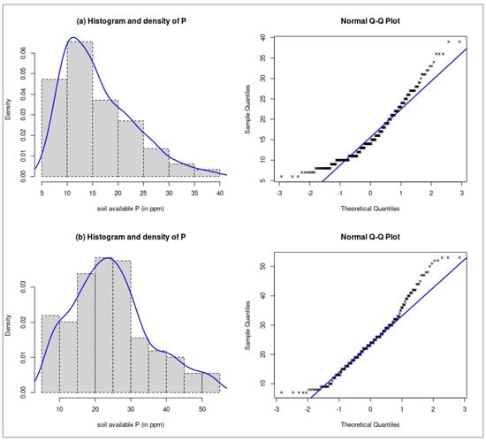
Figure 3.
Histogram and normal Q-Q plot of soil available P within (a) the eastern Ontario and (b) western Ontario zones. Both datasets are approximately normally distributed since data points (denoted with an x) are near the straight reference line.
To understand the shape of the data distribution, we calculated the skew metric and plotted the data distribution for each zone. The eastern Ontario (UTM 18N) zone shows a negative skewness (left-skewed). This indicates the potential prevalence of low soil available p values. On the other hand, the distribution of the western Ontario (UTM 17N) zone dataset is approximatively symmetric, which means that the data points are evenly distributed on both sides of the population mean.
Descriptive statistics of soil available P are detailed in Table 3 for each zone of the study area. The western Ontario zone shows higher soil available P compared with the eastern Ontario zone. The variability of soil available P is higher within the western Ontario zone compared with the eastern Ontario zone. The range of variation and standard deviation for available P were 33 ppm and 46 ppm, and 11 and 7 for the eastern and western Ontario zones, respectively. Higher standard deviation indicates greater variability. This means that the soil available P dataset in the western Ontario zone is more variable than in the eastern zone. Additionally, a smaller standard error was reported in the eastern Ontario zone dataset, indicating that the sample mean is a more precise estimate of the population mean. More confidence in the accuracy of the eastern Ontario zone population mean exists compared with the population mean in the western Ontario zone. Hence, soil available P is characterized by a moderate to high variability across the eastern and western zones, respectively.
Table 3.
Descriptive statistics of soil available P (ppm) within the study area.
3.2. Correlation Relations
Correlation matrices were produced to depict correlation relations between soil available P and obtain insight about potential predictors for soil available P. Correlation matrices were generated, for each UTM zone, based on the calculation of pairwise coefficient of correlation between the predictors and soil available P at p < 0.05 significance level. A hierarchical clustering function was applied to highlight multicollinear variables. A matrix of correlation p-values was calculated to show only significant correlations (Figure 4). Significant coefficients of correlation are shown with redder or bluer color intensities corresponding to stronger positive or negative correlation, respectively.
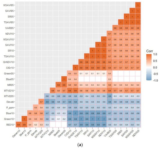
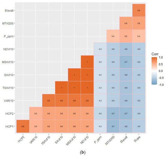
Figure 4.
Correlation matrix of soil available P and auxiliary predictors within (a) eastern Ontario zone and (b) western Ontario zone. Significant coefficient of correlation at p < 0.05 are shown with color intensity changing based on the degree of correlation (significant positive or negative correlation). Correlated predictors are clustered into blocks with similar color intensity to highlight multicollinear features. Insignificant pairwise correlations at the 0.05 level are left blank.
For the eastern Ontario (UTM 18N) zone (Figure 4a), soil available P is significantly (p < 0.05) correlated with the elevation predictor at an r value of 0.5. Soil available P exhibits a positive correlation with RGB bands of the PlanetScope remote sensing data acquired in October, RED10 (r = 0.4), Green10 (r = 0.5), and Blue10 (r = 0.6). Soil available P is also negatively correlated with PlanetScope NIR05 (r = −0.5), Blue05 (r = −0.4), and Green05 (r = −0.4) bands acquired in May. Further, a significant (p < 0.05) negative correlation with soil-vegetation indices, obtained from PlanetScope imagery, is present, varying in r values from r = −0.4 (TSAVI05, SR05, SAVI05, MSAVI05, NDVI05), r = −0.5 (TSAVI10, SR10, SAVI10, MSAVI10, NDVI10, MTVI210, VARI05), to r = −0.6 (ClGr10, GrNDVI10). Soil available P is positively correlated with only the MTVI205 soil-vegetation index index (r = 0.4) within both UTM 18N and 17N zones.
For the western Ontario (UTM 17N) zone (Figure 4b), soil available P is significantly (p < 0.05) correlated with elevation (r = 0.5) and slope (r = 0.4). A significant correlation between soil available P and MTVI205 index (r = 0.4) is present. HCP2 as a PSS variable demonstrates a significant negative correlation with soil available P (r = −0.4). Soil available P is negatively correlated with soil-vegetation indices, including NDVI10, VARI10, SAVI10, and TSAVI10 (r = −0.3). Overall, the degree of correlation between soil available P and all available variables in the UTM 17N zone is weaker compared with results found in the UTM 18N fused dataset.
The elevation predictor is positively correlated with soil available P in both UTM zones. Most vegetation indices are negatively correlated with soil available P and the elevation predictor, which might indicate that lower elevations have higher soil moisture and lower available P than higher elevations.
Correlated soil-vegetation indices and topographic attributes, coming from high-density PSS, the PlanetScope sensor, and high-density geo referentially corrected elevation data, were used to generate geostatistical raster layers of these predictors at 3 m spatial resolution. Figure 5 illustrates examples of PSS and RS raster layers produced for this study. Maps of elevation, PRP2, HCP1, GrNDVI10, and ClGr10 seem to be spatially correlated. Lower elevations generally hold more moisture and produce more biomass than higher elevations. ECa is related to soil water content, which fosters biomass production [82]. Maps of vegetation spectral indices (GrNDVI10 and ClGr10) and ECa (PRP2 and HCP1) reveal the presence of more biomass at lower elevations. This also could justify the prevalence of low soil available values in lower elevations. Further, soil available P, elevation, and pH maps appear to be spatially correlated. Soil pH fluctuates significantly by showing declines in pH values as elevations increase [83]. The positive correlation between soil available P and elevation predictor might be possibly caused by a long-term application of urea-based fertilizers, which tend to increase soil pH [84], and make soil P more available to plants, especially in more acidic soils. This could explain why soil available P increases at higher elevations.
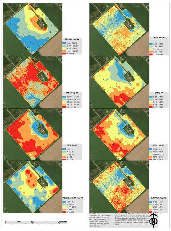
Figure 5.
Example raster layers based on high-density soil sensor readings and PlanetScope remote sensing data at a 3 m resolution in the NX field.
It is worth mentioning how clusters of related variables are organized into groups of either high or low correlation (Figure 4). Overall, including closely related types of features that are either highly or poorly correlated with soil available P should not measurably improve ML model performance. In Section 3.3 and Section 3.4, we explore the results of excluding highly correlated features, in both the western and eastern Ontario zones, to build reliable a predictive machine learning model for soil available P. An RFE algorithm is used to select variables for SVM regressor, and the BART variable selection method is deployed to select powerful predictors for a BART model. Variable selection methods are used to make the learning algorithm faster, select simpler predictive models with fewer features, and improve the interpretability of the selected model.
3.3. Variable Selection
The BART variable selection method reduced the number of predictor variables from forty-two to six or four factors in the eastern and western Ontario zones, respectively. This produces simpler and more interpretable BART models for soil available P. The results of the BART variable selection method show that soil available P is influenced by the important predictors of elevation, Green10, blue05, PRP2, HCP1, and TSAVI05 within fields of the eastern Ontario zone. In western Ontario, soil available P appears to be influenced by the important predictors of elevation, RED10, MTVI205, and FlowDir. The elevation predictor appears to be the most influential feature for both zones (Figure 6). On the other hand, the RFE variable selection method for SVM, which is mainly based on the importance score metric, selected 22 and 15 predictors to produce SVM models for the eastern and western Ontario zones, respectively (Figure 7). These are the optimal number of predictors that can be combined to reach the highest performance for the SVM regressor. However, we observed a huge drop in the performance of SVM models when selecting only 15 and 12 predictors for the eastern and western Ontario zones, respectively. Table 4 summarizes selected predictors for each machine learning method in each Ontario zone.
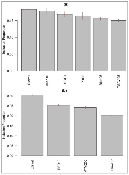
Figure 6.
Selected predictors using the variable inclusion proportions metric of the BART variable selection method. Influential predictors are selected to boost performance of the BART model within (a) eastern zone and (b) western zone.
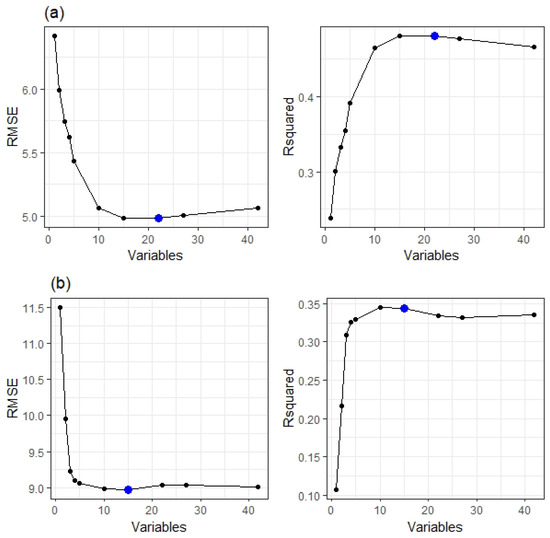
Figure 7.
Variable selection for SVM with RFE algorithm within (a) eastern zone and (b) western zone. To reach the highest R2 and lowest RMSE, 22 and 15 predictors are the optimal number of selected features (denoted using blue dots) within the eastern zone and the western zone, respectively. RMSE and R squared correspond to the training results of SVM models for differing numbers of predictor variables (denoted using black dots) using 10-fold cross-validation.
Table 4.
Results of variable selection methods deployed in this research project. Selected predictors are provided for each machine learning algorithm.
Our results demonstrate that the BART variable selection method performs favorably compared with variable selection with RFE for SVM. We were able to reach lower out-of-sample predictive RMSE values with fewer predictors with BART. Figure 6 illustrates the variable inclusion proportions for selected predictors with the BART variable selection methods in both Ontario zones.
The set of six predictors selected in the eastern Ontario zone by the BART variable selection method are fed to SVM model (SVM6) for comparison between the two variable selection approaches with an equal number of predictor variables. The results show that SVM6 performs better with the BART set of predictors (Table 5). SVM with fifteen predictors was less accurate in predicting soil available P than the SVM model with the six same predictors selected by BART. For example, in the eastern Ontario zone, BART, SVM with 15 predictors, and SVM6 had RMSE values of 5.10, 6.45, and 5.29, respectively. We conclude from this comparison that the RFE variable selection method struggles to detect the most meaningful minimum set of predictors, particularly when dealing with a high dimensional space.
Table 5.
Performance of trained and validated models for fields in the eastern and western Ontario zones (Using regional approach).
BART’s removal of variables that do not improve the accuracy in predicting soil available P helps to increase the interpretability of the resulting predictive models. Most covariates remaining after applying the BART variable selection method are indirectly connected to soil available P. For example, the direction of surface water movement across fields and elevation contribute to the transport of soil P by runoff or erosion. Soil available P is not directly related to ECa; however, factors affecting both soil properties can result in some level of causality. For instance, soil texture, soil moisture, and salinity affect both soil available P and ECa. Further, soil organic matter also influences soil available P and ECa. It controls soil available P by serving as a source of soil nutrients and improving soil structure, which in turn affects retention and release of P. Soil and vegetation indices can be related to soil organic matter and soil carbon using spectral indices from satellite imagery or PSS.
3.4. Model Evaluation
To assess the level of overfitting and select optimal models for soil available P, we derive out-of-sample statistics by using a 10 randomized fold cross-validation method. Supplementary Table S2 provides details about data splitting for regional model development. For BART models, instead of using the default m = 200 for the number of trees, we find the optimal number of trees using the RMSE by number of trees function (Supplementary Figure S2). However, when reducing the number of trees to less than m = 50, the performance of BART selected models are similar and computational time and memory requirement are considerably reduced.
Table 5 summarizes the performance of all trained and validated models with SVM and BART algorithms for both Ontario regions. An optimal model is selected using the largest value of Rsquared and lowest value of RMSE. We obtained reliable posterior mean and interval estimates with BART models having six or four predictors in the eastern or western Ontario zones (RMSE values of 5.1 or 8.86 ppm, respectively). BART performs better than SVM, which has RMSE values of 5.29 and 9.71 for six and twelve predictors in eastern and western Ontario, respectively. No significant improvement in the predictive power of BART was observed in eastern Ontario, while increasing the number of important features from six to twenty-two predictors. Our implementation of BART with the first 22 most important predictors gave an R2 of 0.49 and an RMSE of 5.11ppm. Reducing BART to only six predictors gave an R2 of 0.47 and RMSE of 5.10. The ability to reduce parameters used in the BART models without sacrificing accuracy offers opportunities to select simpler and interpretable spatial predictive BART models for soil available P. Tuned hyperparameters values for BART and SVM models are provided in Table 5.
To compare between the predictive power of OK and BART and SVM, we ran in-field models by splitting the fused regression matrix into seven sub-datasets based on the location of soil samples. Supplementary Table S3 provides details about data splitting for in field model development. Table 6 illustrates results of fitting predictive models with the individual in-field approach. The BART in-field predictive models using separate fused datasets for each field had lower RMSE, higher R2 values, and lower MAE values as compared with predictive models based on SVM and OK, which generally showed prediction accuracies that were relatively similar to each other. BART algorithm improves the predictive performance for soil available P in individual fields, not only exhibiting the lowest RMSE values of 2.18 ppm and 3.58 ppm across the eastern and western Ontario zones, respectively, but also the highest R2 values of 0.85 and 0.83, respectively. In contrast, SVM had RMSE values in the eastern and western Ontario zones, respectively, of 5.04 ppm and 7.51 ppm and R2 values of 0.27 and 0.43 with six and twelve auxiliary predictors. OK RMSE values for soil available P across the eastern and western Ontario zones averaged 4.77 ppm and 7.81 ppm, respectively, while R2 values averaged 0.18 and 0.44. We detected some overfitting with SVM for the NX and LN fields. One of the strategies to reduce overfitting is the application of a suitable variable selection method. However, variable selection improved SVM predictive performance in both fields but was not able to avoid overfitting in the NX field. We also noticed poor validated predictive results within KN and RB fields. This is probably due to the small size of the training and testing datasets of these fields.
Table 6.
Predictive performance of in-field models validated with test datasets (based on 75% training data and 25% testing data).
The predictive performance of OK is not stable across all seven fields. OK works well for some fields (e.g., VN and KN) depending on the sampling density and size. This is also because OK does not consider any auxiliary variables for soil available P prediction. RMSE values for OK available P predictions in eastern Ontario ranged in RMSE values from 2.44 to 6.19. Higher OK RMSE values within western Ontario zone fields were related to the high spatial variability of soil available P within fields of this region. This indicates high uncertainties in the P prediction during the validation of each western Ontario OK field model. Acceptable results from OK were achieved within the LN and HN fields of western Ontario, but with high uncertainties in the predicted values of soil available P. This reduces the reliability of OK in decision-making.
The Ste model (Matern, M. Stein’s parameterization) was optimal in all fields except for the KN field, where a spherical model was optimal (Figure 8 and Figure 9). The best fitting semivariogram models were obtained within VN and KN fields. A moderate spatial structure was obtained in VN and KN, exhibiting the lowest RMSE values of 4.64 and 2.44 pm, respectively. Except for VN and KN fields, the estimated soil available P values exceeded the measured values. Spatial dependence quantifies the degree to which neighboring soil observations are correlated or influencing each other based on the spatial relationship. Nugget to sill ratio measures the degree of spatial dependence. Values for this ratio ranged from 0.16 to 0.59, with the lowest value occurring in field HN. Soil available P reveals a strong spatial dependence within HN field, and moderate spatial dependence within other fields. This indicates a significant spatial correlation, but it might be influenced by other sources of variation or measurement errors.
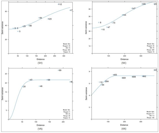
Figure 8.
Experimental and fitted semivariogram models for soil available P within fields of eastern Ontario zone.
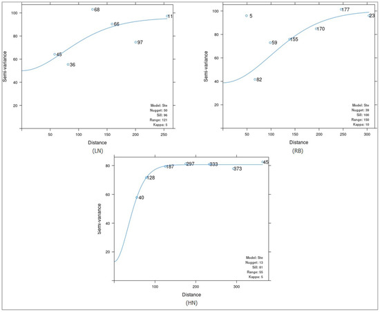
Figure 9.
Experimental and fitted semivariogram models for soil available P within fields of western Ontario zone.
Regional machine learning-based models appear to be the best approach for spatially predicting soil available P, compared with running individual OK models for each field. This approach benefits from including all available soil P observations to train and validate consistent ML models. Region-averaged BART algorithms have better accuracy in predicting soil available P, not only exhibiting the lowest RMSE values of 5.10 ppm and 8.86 ppm across the eastern and western zones, respectively, but also having R2 values of 0.47 and 0.36 within the eastern and western zones, respectively. It is worth mentioning that BART model predictions of soil available P within the eastern zone were particularly promising. RMSE is 3.86 on the training data and 5.10 on the testing data in eastern Ontario, much lower than the RMSE values for corresponding SVM models or for OK RMSE values averaged over all eastern Ontario fields (Table 5 and Table 6). BART performs better because it applies variable selection and explores mutual interaction between predictors. This ensemble ML algorithm performs well when the test of normality for residuals is significant (p-value for Shapiro–Wilk test). BART is an efficient tool for understanding spatial variability in soil available P and improving the accuracy of soil available P predictions within agricultural fields to inform in-field management decisions.
BART requires convergence of its Gibbs sampler, which is a Markov chain Monte Carlo (MCMC) algorithm used to sample from complex high dimensional probability distributions. Four types of convergence diagnostic plots are introduced in Figure 10. By visually checking the convergence diagnostic plots for σ2 by MCMC iteration in the upper left of Figure 10, selected BART models for each Ontario zone have been burned in (after ~250 iteration) and the four plots appear to show a stationary process. Samples on the left of the vertical grey line are burn-ins from the first computing MCMC chain core. Post burn-in iterations are located on the right of the vertical grey line, from the two computing cores used for BART model construction. This plot tracks the estimates of the error variance estimates over the course of the MCMC iterations. The average of σ2 converges to a stable value after the burn-in period (About 250 MCMC iterations), which is good sign of convergence to a stationary value for the BART model. The average of σ2 after burn-in is estimated at 19.00 and 65.14 for the eastern and western zones, respectively. The percentage of trees accepted by MCMC iteration are shown in the top right of Figure 10, where each point refers to one iteration. The vertical line separates the two stages of burn-in and post-burn-in iterations. This plot displays the percentage of tree updates that were accepted at each MCMC iteration. In BART models, tree updates involve changes in the structure of the regression trees, such as splitting or pruning nodes. The acceptance rate of the proposed trees fluctuates in the early iterations. The tree acceptance rate stabilizes as the iterations progress. For both Ontario zones, the percentage of tree acceptance by MCMC iteration converges to a moderate acceptance rate.

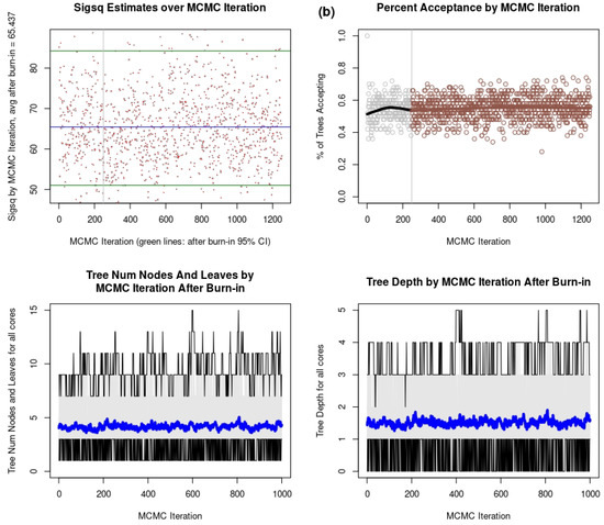
Figure 10.
Convergence diagnostics for BART model within (a) eastern Ontario zone and (b) western Ontario zone.
The average number of leaves across the m trees by MCMC iteration is shown using blue lines at the bottom left of Figure 10. This metric tracks the average number of leaves in the ensemble of regression trees used by the BART model at each MCMC iteration. The average number of leaves varies from three to five for both Ontario zones. The average tree depth of the regression trees within the BART model ensemble at each MCMC iteration is shown at the bottom right of Figure 8. The average tree depth is in the range of 1 to 2 for both Ontario zones. A stable average number of leaves and tree depth indicate that the tree structure has settled down and is not changing dramatically. Stable and consistent values are indicative of good convergence. The BART model is efficiently sampling from the posterior distribution.
4. Discussion
Previous studies that predicted spatially variable soil available P were compared with the results of the present study. Random forest (RF) was used previously by Saifuzzaman [49] to spatially predict soil available P for the LN field also evaluated in the present study. For the LN field, the accuracy of soil available P predictions was better with BART (RMSE = 3.27) in the present study than with RF (RMSE = 4.82) in the Saifuzzaman [49] study. In Saifuzzaman [49], however, the RF model for soil P in the LN field was based on a combination of fifteen predictors (including gamma ray sensing data not used in the present study), whereas the BART model in the present study had only four predictors. In both studies, topographic attributes, ECa and NDVI, were important predictors, but additional remote sensing-based predictors not used by Saifuzzaman [49] were also important in the present study.
In a separate study, conducted in South Korea by Jeong et al., 2017 [37], RF was used with soil and vegetation spectral indices to predict phosphorus at the regional scale with an RMSE of 120, which is much higher compared with RMSE values of less than 5 with BART in the present study at the regional scale. The higher RMSE in study [37] is likely due to the large variability in measured soil phosphorus, which ranged from 5 to 300 ppm.
The present study is an attempt to develop regional models for seven different spatially clustered fields in two regions of Ontario. A novel approach of developing predictive models for clusters of fields shows promising results for soil available P spatial prediction. The optimal number of predictors should be determined to extract the most useful information from the fused dataset, which could help deal with the challenging question of improving the prediction of soil available P. Determining the best combination of predictors leads to an optimal predictive performance of selected models. A significant improvement in the coefficient of determination and RMSE was noticed when predictors with low importance were suppressed.
One of the drawbacks of SVM is its computational cost, particularly when dealing with large datasets. SVM failed to detect the best set of features that could help in reaching higher predictive performance and building simpler and interpretable SVM models for soil available P. SVM also requires data preprocessing, such as normalization and feature scaling, to ensure optimal performance.
On the other hand, there are several strengths of BART. High predictive performance was achieved with the BART algorithm. BART models offer several advantages over traditional regression methods, including the ability to model complex non-linear relationships, account for interactions between variables, and incorporate prior information through Bayesian inference. Additionally, BART models have built-in uncertainty estimates, which can be used to quantify the prediction errors and lead to predictions that are more robust. The sum of trees and the regularization of prior distributions are the two core steps that distinguish BART models. The convergence of BART’s MCMC chain is designed to identify non-linearity and flexibly fit tree-based models. In summary, BART implicitly performs variable selection by considering the inclusion or exclusion of predictors during the tree-building process. Variables that are more informative for soil available P are more likely to be included in the model, while less relevant variables are excluded. This results in an ensemble of trees that collectively model the relationship between predictors and soil available P while automatically selecting the most relevant variables.
BART predictive performance within the eastern Ontario zone is much higher compared with the western Ontario zone. This may be due to the high spatial variability of soil available P within the western zone, distance between fields and the soil sampling protocol (Table 5). Partial Dependence Plots (PDPs) [85] were used to explore how selected predictors affect soil available P prediction. PDPs are used as an exploratory tool to understand relationships between selected predictors and soil available P. PDPs are a useful tool for visualizing these relationships and illustrating the marginal effect of each selected predictor on soil available P.
Figure 11 and Figure 12 show PDPs illustrating the main effect of each selected feature on the predicted values of soil available P. Non-linearity between selected predictors and soil available P is detected in both zones. Selected predictors show moderate to strong non-linear partial effects. The marginal effect of selected predictors within the western Ontario zone is more significant compared with those selected predictors for the eastern zone. Although the elevation predictor was the most influential feature in both zones, the amplitude of variation in the marginal effect of the elevation predictor is equal to 14 within the eastern Ontario zone and 28 within the western Ontario zone.
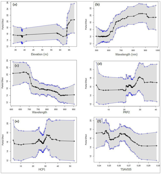
Figure 11.
PDP plots to explore the sensitivity of selected features (a) Elevation, (b) Green10 Wavelength, (c) Blue05 Wavelength, (d) PRP2, (e) HCP1, and (f) TSAVI05 on soil available P prediction. PDPs plotted in black dots and corresponding line and 95% credible upper and lower intervals plotted in blue dots and corresponding lines for six predictors in the eastern Ontario zone.
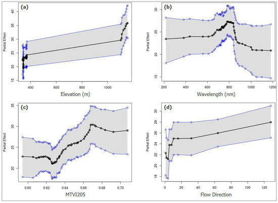
Figure 12.
PDP plots to explore the sensitivity of BART selected features (a) Elevation, (b) Red10 wavelength, (c) MTVI205, and (d) Flow Direction on soil available P prediction. PDPs plotted in black dots and line and 95% credible upper and lower intervals plotted in blue dots and lines for four predictors in the western Ontario zone.
In the eastern Ontario zone, a sudden drop in the marginal effect of the elevation predictor on the predicted values of soil available P was detected around 38 m and 60–65 m (Figure 11a). In the western Ontario zone, a sudden drop in the marginal effect of elevation on soil available P occurred around 380 m, while a positive relationship and significant effect on the model’s prediction accuracy occurred at around 1100 m (Figure 12a).
To determine sensitive wavelengths from PlanetScope RS data, we used PDPs to measure the average marginal effect of selected features on predicted values of soil available P. According to PDPs in Figure 11b,c and Figure 12b, bands of PlanetScope remote sensing data indicate wavelengths that have predictive power for soil available P or auxiliary variables that may indirectly control soil available P. Wavelengths in the 650–700 nm and 800–900 nm regions of the electromagnetic spectrum are particularly relevant to soil available P concentration. On the other hand, the TSAVI index, calculated from PlanetScope RS data, influences soil available P prediction in the 0.245–0.27 values of this soil index (Figure 11f). A drop and significant positive marginal effect of MTVI205 index on soil available P occurred in the range of 0.62–0.67 (Figure 12c).
Apparent electrical conductivity (ECa) is useful for the prediction of soil available P. Two sharp rises were noticed around 22 and 30 for PRP2 feature. In contrast, HCP1 influences soil available P prediction around the 25–35 ECa range. Therefore, ECa values around the 22–35 range influence the average marginal effect of soil available P (Figure 11d,e).
Beyond detecting non-linearity between soil available P and selected predictors, we transformed the BART model to a simpler and interpretable decision tool. We are able to understand the behavior of each predictor by detecting the overall trend, sharp changes or sudden drops or rises. This can indicate interactions or thresholds where a specific feature has a significant effect on the model’s prediction.
5. Conclusions
The spatial prediction of soil available P is challenging due to high spatial variability and nonlinearity. BART, SVM, and OK models were compared using ground truth data on soil available P from seven commercial farms in Ontario, Canada and an initial set of 42 auxiliary predictors, including primary and secondary terrain attributes, and proximal and satellite remote sensing data. BART models with only four–six auxiliary predictors outperformed SVM and OK modeling methods for soil available P in both eastern and western Ontario farm cluster zones. BART modeling resulted in excellent out-of sample predictive performance for the spatial prediction of soil available P. For better P fertilizer decision-making, advanced machine learning tools applied to auxiliary predictors can be used to assess the spatial variability of soil available P. Variable selection and the inclusion of other types of auxiliary predictors, such as in-field management practices, is advisable to improve the prediction accuracy of soil available P. The application of BART to predict soil available P revealed a variety of appealing features. This algorithm is computationally inexpensive and provides a set of tools for machine learning visualization. Features of BART, such as prediction, variable selection, and interaction, are parallelized across multiple and customized computing processors or cores. Parallel processing is needed to perform complex computations, particularly with larger ensembles and deeper trees. BART can be particularly useful when dealing with high-dimensional data or complex non-linear relationships between variables, as it can effectively identify which predictors are important for making accurate predictions. To investigate the effect of selected features on model predictions, we used PDPs as an exploratory tool to visualize the relationship between selected predictors and soil available P. We demonstrate that PDPs are a valuable tool for interpreting the behavior of each selected predictor and visualizing the relationship between selected predictors and soil available P. PDPs help understand how individual features influence the BART prediction of soil available P. PDPs show how soil available P predictions change as the feature of interest varies over its marginal distribution, while all other features are held constant. Hence, we recovered complex relationships between soil available P and selected features.
Supplementary Materials
The following supporting information can be downloaded at: https://www.mdpi.com/article/10.3390/agronomy14040693/s1, Table S1. Details of the fields considered in this research project, including size of the fields, number of soil samples, Proximal Soil Sampling (PSS) variables, number of PSS readings and acronyms for predictive models based on the geographic zone where fields are located. Dualem measured horizontal coplanar geometry-HCP and perpendicular geometry-PRP ECa, each at two depths (1 and 2). Table S2. Data splitting for regional and global models. Table S3. Data splitting for in-field models. Figure S1. Normality test of errors using Q-Q plot and the Shapiro-Wilk test, residual plot to assess heteroscedasticity within (a) eastern Ontario (UTM 18N) zone and (b) western Ontario (UTM 17N) zone. There is little evidence of the errors violating normality and homoscedasticity. Figure S2. Optimization of the number of trees with the out-of-sample RMSE for (a) eastern Ontario (UTM 18N) zone and (b) western Ontario (UTM 17N) zone.
Author Contributions
Conceptualization, A.L. and D.J.M.; Data acquisition and curation, A.L. and V.A.; Formal analysis, A.L.; Funding acquisition, D.J.M.; Methodology, A.L; Project administration, D.J.M.; Software, A.L; Supervision, D.J.M.; Validation, A.L. and D.J.M.; Visualization, A.L. and D.J.M.; Writing—original, A.L.; Writing—review and editing, A.L., D.J.M. and V.A. All authors have read and agreed to the published version of the manuscript.
Funding
This research project was funded by the Mohamed VI Polytechnic University (UM6P) in Morocco. Data collection was supported in part through the development of scale-up sensor-based precision agriculture services in Ontario project MD-2014-2487 funded by the Ontario Ministry of Agriculture, Food and Rural Affairs (OMAFRA) through the New Directions Research Program (NDRP).
Data Availability Statement
Restrictions apply to the availability of these data. Data were obtained from the Ontario Ministry of Agriculture, Food and Rural Affairs (OMAFRA) and are available from the authors with the permission of OMAFRA.
Acknowledgments
We acknowledge the contribution of Faouzi Bekkaoui (INRA, Morocco), Abdallah Oukerroum (UM6P), John Vreyens (University of Minnesota), and David Mulla (University of Minnesota) to establish an exchange scholar-visiting program between the University of Minnesota and the Mohamed VI Polytechnic University in Morocco. We gratefully acknowledge the support of Viacheslav Adamchuk and Md Saifuzzaman by providing soil samples and PSS data from Ontario. We appreciate the critical and constructive comments from the reviewers, which helped improve the quality of this manuscript.
Conflicts of Interest
The authors declare no conflicts of interest.
References
- Irfan, M.; Aziz, T.; Maqsood, M.A.; Bilal, H.M.; Siddique, K.H.M.; Xu, M. Phosphorus (P) use efficiency in rice is linked to tissue-specific biomass and P allocation patterns. Sci. Rep. 2020, 10, 4278. [Google Scholar] [CrossRef]
- FAO. Feeding the World in 2050—FAO. Available online: https://www.google.com.sg/url?sa=t&source=web&rct=j&opi=89978449&url=https://www.fao.org/fileadmin/templates/wsfs/Summit/WSFS_Issues_papers/WSFS_feeding_E.pdf&ved=2ahUKEwjhstiP7ZiFAxUMklYBHdFUDMsQFnoECBQQAQ&usg=AOvVaw1mGxw7dVrAEgvVEkT0Rl6V (accessed on 31 January 2024).
- Mahdi, S.S.; Talat, M.A.; Dar, M.H.; Hamid, A.; Ahmad, L. Soil phosphorus fixation chemistry and role of phosphate solubilizing bacteria in enhancing its efficiency for sustainable cropping—A review. J. Pure Appl. Microbiol. 2012, 6, 1905–1911. [Google Scholar]
- Simard, R.R.; Nolin, M.C.; Cambouris, A.N. Application of Precision Farming to Potato Production in Québec. Better Crops 1998, 82, 22–24. Available online: https://ucanr.edu/sites/nm/files/76650.pdf (accessed on 1 March 2023).
- Mulla, D.J.; Schepers, J.S. Key Processes and Properties for Site-Specific Soil and Crop Management. In The State of Site Specific Management for Agriculture; Wiley: Hoboken, NJ, USA, 2015; pp. 1–18. [Google Scholar] [CrossRef]
- Zhu, H.X.; Chen, X.M. Spatial variability of soil phosphorus based on geostatistics. In Proceedings of the 2010 International Conference on Multimedia Technology, Hong Kong, China, 28–30 December 2010. [Google Scholar] [CrossRef]
- Fang, F.; Brezonik, P.L.; Mulla, D.J.; Hatch, L.K. Estimating Runoff Phosphorus Losses from Calcareous Soils in the Minnesota River Basin. J. Environ. Qual. 2002, 31, 1918–1929. [Google Scholar] [CrossRef]
- Miao, Y.; Mulla, D.J.; Robert, P.C. An integrated approach to site-specific management zone delineation. Front. Agric. Sci. Eng. 2018, 5, 432–441. [Google Scholar] [CrossRef]
- Mulla, D. Using Geostatistics and GIS to Manage Spatial Patterns in Soil Fertility. In Proceedings of the 1991 Symposium, Chicago, IL, USA, 16–17 December 1991; Available online: https://experts.umn.edu/en/publications/using-geostatistics-and-gis-to-manage-spatial-patterns-in-soil-fe (accessed on 2 March 2023).
- Mulla, D.J. Mapping and Managing Spatial Patterns in Soil Fertility and Crop Yield. In Soil Specific Crop Management: A Workshop on Research and Development Issues; American Society of Agronomy, Crop Science Society of America, Soil Science Society of America: Madison, WI, USA, 1993. [Google Scholar] [CrossRef]
- Nawar, S.; Corstanje, R.; Halcro, G.; Mulla, D.; Mouazen, A.M. Delineation of Soil Management Zones for Variable-Rate Fertilization: A Review, 1st ed.; Elsevier Inc.: Amsterdam, The Netherlands, 2017; Volume 143. [Google Scholar] [CrossRef]
- Sinfield, J.V.; Fagerman, D.; Colic, O. Evaluation of sensing technologies for on-the-go detection of macro-nutrients in cultivated soils. Comput. Electron. Agric. 2010, 70, 1–18. [Google Scholar] [CrossRef]
- Adamchuk, V.I.; Rossel, R.V.; Sudduth, K.A.; Lammers, P.S. Sensor Fusion for Precision Agriculture. Sens. Fusion-Found. Appl. 2011, 13, 27–40. [Google Scholar] [CrossRef]
- Dong, X.L.; Rekatsinas, T. Data integration and machine learning: A natural synergy. In Proceedings of the 2018 International Conference on Management of Data, Houston, TX, USA, 10–15 June 2018; pp. 1645–1650. [Google Scholar] [CrossRef]
- Mulder, V.L.; de Bruin, S.; Schaepman, M.E.; Mayr, T.R. The use of remote sensing in soil and terrain mapping—A review. Geoderma 2011, 162, 1–19. [Google Scholar] [CrossRef]
- Souza, E.G.; Bazzi, C.L.; Khosla, R.; Uribe-Opazo, M.A.; Reich, R.M. Interpolation type and data computation of crop yield maps is important for precision crop production. J. Plant Nutr. 2016, 39, 531–538. [Google Scholar] [CrossRef]
- Yao, R.J.; Yang, J.S.; Wu, D.H.; Xie, W.P.; Gao, P.; Wang, X.P. Characterizing spatial–temporal changes of soil and crop parameters for precision management in a coastal rainfed agroecosystem. Agron. J. 2016, 108, 2462–2477. [Google Scholar] [CrossRef]
- Shi, H.; Hellwich, O.; Luo, G.; Chen, C.; He, H.; Ochege, F.U.; Van De Voorde, T.; Kurban, A.; De Maeyer, P. A Global Meta-Analysis of Soil Salinity Prediction Integrating Satellite Remote Sensing, Soil Sampling, and Machine Learning. IEEE Trans. Geosci. Remote Sens. 2022, 60, 1–5. [Google Scholar] [CrossRef]
- Houborg, R.; McCabe, M.F. High-Resolution NDVI from Planet’s Constellation of Earth Observing Nano-Satellites: A New Data Source for Precision Agriculture. Remote Sens. 2016, 8, 768. [Google Scholar] [CrossRef]
- Asner, G.P.; Martin, R.E.; Mascaro, J. Coral reef atoll assessment in the South China Sea using Planet Dove satellites. Remote Sens. Ecol. Conserv. 2017, 3, 57–65. [Google Scholar] [CrossRef]
- Moody, D.I.; Bauer, D.E.; Brumby, S.P.; Chisolm, E.D.; Warren, M.S.; Skillman, S.W.; Keisler, R. Land cover classification in fused multisensor multispectral satellite imagery. In Proceedings of the 2016 IEEE Southwest Symposium on Image Analysis and Interpretation (SSIAI), Albuquerque, NM, USA, 29–31 March 2016; pp. 85–88. [Google Scholar] [CrossRef]
- Fu, P.; Vintila, R.; Tan, J.; Ding, J.; Han, L.; Ge, X.; Wang, X.; Wang, J.; Wang, R.; Qin, S.; et al. Exploring PlanetScope Satellite Capabilities for Soil Salinity Estimation and Mapping in Arid Regions Oases. Remote Sens. 2023, 15, 1066. [Google Scholar] [CrossRef]
- Kpienbaareh, D.; Sun, X.; Wang, J.; Luginaah, I.; Kerr, R.B.; Lupafya, E.; Dakishoni, L. Crop Type and Land Cover Mapping in Northern Malawi Using the Integration of Sentinel-1, Sentinel-2, and PlanetScope Satellite Data. Remote Sens. 2021, 13, 700. [Google Scholar] [CrossRef]
- Sadeh, Y.; Zhu, X.; Dunkerley, D.; Walker, J.P.; Zhang, Y.; Rozenstein, O.; Manivasagam, V.S.; Chenu, K. Fusion of Sentinel-2 and PlanetScope time-series data into daily 3 m surface reflectance and wheat LAI monitoring. Int. J. Appl. Earth Obs. Geoinf. 2021, 96, 102260. [Google Scholar] [CrossRef]
- Silvero, N.E.; Demattê, J.A.; Vieira, J.d.S.; Mello, F.A.d.O.; Amorim, M.T.A.; Poppiel, R.R.; Mendes, W.d.S.; Bonfatti, B.R. Soil property maps with satellite images at multiple scales and its impact on management and classification. Geoderma 2021, 397, 115089. [Google Scholar] [CrossRef]
- Koparan, M. Estimating Soil Organic Carbon in Cultivated Soils Using Soil Test Data, Remote Sensing Imagery from Satellites (Landsat 8 and PlantScope), and Web Soil Survey Data. Master’s Thesis, South Dakota State University, Brookings, SD, USA, 2019. Available online: https://openprairie.sdstate.edu/etd/3177 (accessed on 27 February 2023).
- Bouasria, A.; Namr, K.I.; Rahimi, A.; Ettachfini, E.M. Geospatial Assessment of Soil Organic Matter Variability at Sidi Bennour District in Doukkala Plain in Morocco. J. Ecol. Eng. 2021, 22, 120–130. [Google Scholar] [CrossRef] [PubMed]
- Zhang, S.; Huang, Y.; Shen, C.; Ye, H.; Du, Y. Spatial prediction of soil organic matter using terrain indices and categorical variables as auxiliary information. Geoderma 2012, 171–172, 35–43. [Google Scholar] [CrossRef]
- Hengl, T.; Heuvelink, G.B.M.; Rossiter, D.G. About regression-kriging: From equations to case studies. Comput. Geosci. 2007, 33, 1301–1315. [Google Scholar] [CrossRef]
- Hengl, T.; Heuvelink, G.B.M.; Stein, A. A generic framework for spatial prediction of soil variables based on regression-kriging. Geoderma 2004, 120, 75–93. [Google Scholar] [CrossRef]
- Sun, W.; Minasny, B.; McBratney, A. Analysis and prediction of soil properties using local regression-kriging. Geoderma 2012, 171, 16–23. [Google Scholar] [CrossRef]
- Wadoux, A.M.J.C.; Minasny, B.; McBratney, A.B. Machine learning for digital soil mapping: Applications, challenges and suggested solutions. Earth-Sci. Rev. 2020, 210, 103359. [Google Scholar] [CrossRef]
- Cressie, N.; Johannesson, G. Fixed rank kriging for very large spatial data sets. J. R. Stat. Soc. Ser. B 2008, 70, 209–226. [Google Scholar] [CrossRef]
- Li, Q.Q.; Wang, C.Q.; Zhang, W.J.; Yu, Y.; Li, B.; Yang, J.; Bai, G.C.; Cai, Y. Prediction of soil nutrients spatial distribution based on neural network model combined with goestatistics. J. Appl. Ecol. 2013, 24, 459–466. Available online: https://europepmc.org/article/med/23705392 (accessed on 8 March 2023).
- Komariah; Husnan; Mujiyo; Suryono. The accuracy of PlanetScope imagery to nitrogen, phosphorus, potassium and sulfur nutrition estimation in terraced paddy field. Int. J. Agric. Res. Innov. Technol. 2021, 11, 1–9. [Google Scholar] [CrossRef]
- Forkuor, G.; Hounkpatin, O.K.L.; Welp, G.; Thiel, M. High resolution mapping of soil properties using Remote Sensing variables in south-western Burkina Faso: A comparison of machine learning and multiple linear regression models. PLoS ONE 2017, 12, e0170478. [Google Scholar] [CrossRef] [PubMed]
- Jeong, G.; Oeverdieck, H.; Park, S.J.; Huwe, B.; Ließ, M. Spatial soil nutrients prediction using three supervised learning methods for assessment of land potentials in complex terrain. CATENA 2017, 154, 73–84. [Google Scholar] [CrossRef]
- Song, Y.; Zhao, X.; Su, H.; Li, B.; Hu, Y.; Cui, X. Predicting Spatial Variations in Soil Nutrients with Hyperspectral Remote Sensing at Regional Scale. Sensors 2018, 18, 3086. [Google Scholar] [CrossRef]
- Hengl, T.; Leenaars, J.G.B.; Shepherd, K.D.; Walsh, M.G.; Heuvelink, G.B.M.; Mamo, T.; Tilahun, H.; Berkhout, E.; Cooper, M.; Fegraus, E.; et al. Soil nutrient maps of Sub-Saharan Africa: Assessment of soil nutrient content at 250 m spatial resolution using machine learning. Nutr. Cycl. Agroecosystems 2017, 109, 77–102. [Google Scholar] [CrossRef]
- Heung, B.; Ho, H.C.; Zhang, J.; Knudby, A.; Bulmer, C.E.; Schmidt, M.G. An overview and comparison of machine-learning techniques for classification purposes in digital soil mapping. Geoderma 2016, 265, 62–77. [Google Scholar] [CrossRef]
- Kaya, F.; Başayiğit, L.; Keshavarzi, A.; Francaviglia, R. Digital mapping for soil texture class prediction in northwestern Türkiye by different machine learning algorithms. Geoderma Reg. 2022, 31, e00584. [Google Scholar] [CrossRef]
- Helfenstein, A.; Mulder, V.L.; Heuvelink, G.B.M.; Okx, J.P. Tier 4 maps of soil pH at 25 m resolution for the Netherlands. Geoderma 2022, 410, 115659. [Google Scholar] [CrossRef]
- Naimi, S.; Ayoubi, S.; Demattê, J.A.M.; Zeraatpisheh, M.; Amorim, M.T.A.; Mello, F.A.d.O. Spatial prediction of soil surface properties in an arid region using synthetic soil image and machine learning. Geocarto Int. 2021, 37, 8230–8253. [Google Scholar] [CrossRef]
- Hengl, T.; Heuvelink, G.B.M.; Kempen, B.; Leenaars, J.G.B.; Walsh, M.G.; Shepherd, K.D.; Sila, A.; MacMillan, R.A.; De Jesus, J.M.; Tamene, L.; et al. Mapping soil properties of Africa at 250 m resolution: Random forests significantly improve current predictions. PLoS ONE 2015, 10, e0125814. [Google Scholar] [CrossRef]
- Hengl, T.; Miller, M.A.E.; Križan, J.; Shepherd, K.D.; Sila, A.; Kilibarda, M.; Antonijević, O.; Glušica, L.; Dobermann, A.; Haefele, S.M.; et al. African soil properties and nutrients mapped at 30 m spatial resolution using two-scale ensemble machine learning. Sci. Rep. 2021, 11, 6130. [Google Scholar] [CrossRef] [PubMed]
- Zhang, X.; Xue, J.; Xiao, Y.; Shi, Z.; Chen, S. Towards Optimal Variable Selection Methods for Soil Property Prediction Using a Regional Soil Vis-NIR Spectral Library. Remote Sens. 2023, 15, 465. [Google Scholar] [CrossRef]
- Sahabiev, I.; Smirnova, E.; Giniyatullin, K. Spatial Prediction of Agrochemical Properties on the Scale of a Single Field Using Machine Learning Methods Based on Remote Sensing Data. Agronomy 2021, 11, 2266. [Google Scholar] [CrossRef]
- Matinfar, H.R.; Maghsodi, Z.; Mousavi, S.R.; Rahmani, A. Evaluation and Prediction of Topsoil organic carbon using Machine learning and hybrid models at a Field-scale. CATENA 2021, 202, 105258. [Google Scholar] [CrossRef]
- Saifuzzaman, M. Optimization of Geospatial Data Modelling for Crop Production by Integrating Proximal Soil Sensing and Remote Sensing Data; McGill University: Montreal, QC, USA, 2020; Available online: https://escholarship.mcgill.ca/concern/theses/05741x41m (accessed on 31 January 2024).
- Wadoux, A.M.J.C.; Samuel-Rosa, A.; Poggio, L.; Mulder, V.L. A note on knowledge discovery and machine learning in digital soil mapping. Eur. J. Soil Sci. 2020, 71, 133–136. [Google Scholar] [CrossRef]
- Heck, R.; Warren, J.; Saurette, D. SOILS OF ONTARIO. Available online: https://openpress.usask.ca/soilscience/chapter/soils-of-ontario/ (accessed on 19 December 2023).
- ESRI. Arcgis Pro; Environmental Systems Research Institute: Redlands, CA, USA, 2022. [Google Scholar]
- Jenson, S.K.; Domingue, J.O. Extracting topographic structure from digital elevation data for geographic information-system analysis. Photogramm. Eng. Remote Sens. 1988, 54, 1593–1600. [Google Scholar]
- Zevenbergen, L.W.; Thorne, C.R. Quantitative analysis of land surface topography. Earth Surf. Process. Landf. 1987, 12, 47–56. [Google Scholar] [CrossRef]
- Wilson, J.; Gallant, J. Secondary Topographic Attributes; John Wiley and Sons: New York, NY, USA, 2000. [Google Scholar]
- Moore, I.D.; Grayson, R.B.; Ladson, A.R. Digital terrain modelling: A review of hydrological, geomorphological, and biological applications. Hydrol. Process. 1991, 5, 3–30. [Google Scholar] [CrossRef]
- Moore, I.D.; Wilson, J.P. Length-slope factors for the Revised Universal Soil Loss Equation: Simplified method of estimation. J. Soil Water Conserv. 1992, 47, 423–428. Available online: https://www.jswconline.org/content/47/5/423 (accessed on 18 February 2023).
- Planet Team. Planetscope. Interface: In Space for Life on Earth; Planet Application Program: San Francisco, CA, USA, 2023; Available online: https://api.planet.com (accessed on 31 January 2024).
- Planet. PlanetScope Product Specifications. 2023. Available online: https://assets.planet.com/docs/Planet_PSScene_Imagery_Product_Spec_letter_screen.pdf (accessed on 31 January 2024).
- Rouse, J.W.J.; Haas, R.H.; Schell, J.A.; Deering, D.W. Monitoring Vegetation Systems in the Great Plains with ERTS; NASA. Goddard Sp. Flight Cent. 3d ERTS-1 Symp; NASA Spec. Publ.: Washington, DC, USA, 1974; Volume 1. [Google Scholar]
- Gitelson, A.A.; Kaufman, Y.J.; Merzlyak, M.N. Use of a green channel in remote sensing of global vegetation from EOS-MODIS. Remote Sens. Environ. 1996, 58, 289–298. [Google Scholar] [CrossRef]
- Huete, A.R. A soil-adjusted vegetation index (SAVI). Remote Sens. Environ. 1988, 25, 295–309. [Google Scholar] [CrossRef]
- Baret, F.; Guyot, G. Potentials and limits of vegetation indices for LAI and APAR assessment. Remote Sens. Environ. 1991, 35, 161–173. [Google Scholar] [CrossRef]
- Qi, J.; Chehbouni, A.; Huete, A.R.; Kerr, Y.H.; Sorooshian, S. A modified soil adjusted vegetation index. Remote Sens. Environ. 1994, 48, 119–126. [Google Scholar] [CrossRef]
- Gitelson, A.A.; Kaufman, Y.J.; Stark, R.; Rundquist, D. Novel algorithms for remote estimation of vegetation fraction. Remote Sens. Environ. 2002, 80, 76–87. [Google Scholar] [CrossRef]
- Birth, G.S.; McVey, G.R. Measuring the Color of Growing Turf with a Reflectance Spectrophotometer1. Agron. J. 1968, 60, 640–643. [Google Scholar] [CrossRef]
- Haboudane, D.; Miller, J.R.; Tremblay, N.; Zarco-Tejada, P.J.; Dextraze, L. Integrated narrow-band vegetation indices for prediction of crop chlorophyll content for application to precision agriculture. Remote Sens. Environ. 2002, 81, 416–426. [Google Scholar] [CrossRef]
- Kuhn, M. R Package “caret” Classification and Regression Training. 2022. Available online: https://scholar.googleusercontent.com/scholar?q=cache:ocTYHTbYAvoJ:scholar.google.com/+R+Package+%E2%80%9Ccaret%E2%80%9D+Classification+and+Regression+Training&hl=ja&as_sdt=0,5&as_vis=1 (accessed on 18 February 2023).
- Kuhn, M. Building predictive models in R using the caret package. J. Stat. Softw. 2008, 28, 1–26. [Google Scholar] [CrossRef]
- RStudio Team. RStudio. RStudio: Integrated Development for R; RStudio, PBC: Boston, MA, USA, 2022. [Google Scholar]
- Kapelner, A.; Bleich, J. bartMachine: Machine Learning with Bayesian Additive Regression Trees. J. Stat. Softw. 2016, 70, 1–40. [Google Scholar] [CrossRef]
- Simon, U. Package ‘rJava’, Low-Level R to Java Interface. 2022. Available online: http://www.rforge.net/rJava/ (accessed on 18 February 2023).
- Chipman, H.A.; George, E.I.; Mcculloch, R.E. BART: Bayesian Additive Regression Trees. Ann. Appl. Stat. 2010, 4, 266–298. [Google Scholar] [CrossRef]
- Hill, J.; Linero, A.; Murray, J. Bayesian additive regression trees: A review and look forward. Annu. Rev. Stat. Appl. 2020, 7, 251–278. [Google Scholar] [CrossRef]
- Hastie, T.; Tibshirani, R. Bayesian backfitting (with comments and a rejoinder by the authors. Stat. Sci. 2000, 15, 196–223. [Google Scholar] [CrossRef]
- Cortes, C.; Vapnik, V.; Saitta, L. Support-vector networks. Mach. Learn. 1995, 20, 273–297. [Google Scholar] [CrossRef]
- Powell, M.J.D. Restart procedures for the conjugate gradient method. Math. Program. 1977, 12, 241–254. [Google Scholar] [CrossRef]
- Isaaks, E.H.; Srivastava, R.M. An Introduction to Applied Geostatistics; Oxford University Press: New York, NY, USA, 1989. [Google Scholar]
- Hiemstra, P.; Hiemstra, M.P. Package ‘automap’. Compare 2013, 105, 10. [Google Scholar]
- Pebesma, E.J. Multivariable geostatistics in S: The gstat package. Comput. Geosci. 2004, 30, 683–691. [Google Scholar] [CrossRef]
- Guyon, I.; Weston, J.; Barnhill, S.; Vapnik, V. Gene selection for cancer classification using support vector machines. Mach. Learn. 2002, 46, 389–422. [Google Scholar] [CrossRef]
- Ratshiedana, P.E.; Elbasit, M.A.M.A.; Adam, E.; Chirima, J.G.; Liu, G.; Economon, E.B. Determination of Soil Electrical Conductivity and Moisture on Different Soil Layers Using Electromagnetic Techniques in Irrigated Arid Environments in South Africa. Water 2023, 15, 1911. [Google Scholar] [CrossRef]
- Mangral, Z.A.; Islam, S.U.; Tariq, L.; Kaur, S.; Ahmad, R.; Malik, A.H.; Goel, S.; Baishya, R.; Barik, S.K.; Dar, T.U.H. Altitudinal gradient drives significant changes in soil physico-chemical and eco-physiological properties of Rhododendron anthopogon: A case study from Himalaya. Front. For. Glob. Chang. 2023, 6, 1181299. [Google Scholar] [CrossRef]
- Rochette, P.; Angers, D.A.; Chantigny, M.H.; Gasser, M.-O.; MacDonald, J.D.; Pelster, D.E.; Bertrand, N. NH3 volatilization, soil concentration and soil pH following subsurface banding of urea at increasing rates. Can. J. Soil Sci. 2013, 93, 261–268. [Google Scholar] [CrossRef]
- Friedman, J.H. Greedy function approximation: A gradient boosting machine. Ann. Stat. 2001, 29, 1189–1232. [Google Scholar] [CrossRef]
Disclaimer/Publisher’s Note: The statements, opinions and data contained in all publications are solely those of the individual author(s) and contributor(s) and not of MDPI and/or the editor(s). MDPI and/or the editor(s) disclaim responsibility for any injury to people or property resulting from any ideas, methods, instructions or products referred to in the content. |
© 2024 by the authors. Licensee MDPI, Basel, Switzerland. This article is an open access article distributed under the terms and conditions of the Creative Commons Attribution (CC BY) license (https://creativecommons.org/licenses/by/4.0/).