Inversion of Soil Salinity in the Irrigated Region along the Southern Bank of the Yellow River Using UAV Multispectral Remote Sensing

Abstract

Soil salinization is a global issue confronting humanity, imposing significant constraints on agricultural production in the irrigated regions along the southern bank of the Yellow River. This, in turn, leads to the degradation of the ecological environment and inadequate grain yields. Hence, it is essential to explore the magnitude and spatial patterns of soil salinization to promote efficient and sustainable agricultural development. This study carried out a two-year surface soil sampling experiment encompassing the periods before spring irrigation and the budding, flowering, and maturity stages of sunflower fields in the irrigated area along the southern bank of the Yellow River. It employed deep learning in conjunction with multispectral remote sensing conducted by UAV to estimate soil salinity levels in the sunflower fields. Following the identification of sensitive spectral variables through correlation analysis, we proceeded to model and compare the accuracy and stability of various models, including the deep learning Transformer model, traditional machine learning BP neural network (BPNN), random forest model (RF), and partial least squares regression model (PLSR). The findings indicate that the precision of soil salinity content (SSC) retrieval in saline–alkali land can be significantly enhanced by incorporating the RE band of UAV data. Four SSC inversion models were developed using the most suitable spectral variables, resulting in precise soil salinity inversion. The model order based on accuracy and stability was Transformer > BPNN > RF > PLSR. Notably, the Transformer model achieved a prediction accuracy exceeding 0.8 for both the training and test datasets, as indicated by R² values. The precision order of the soil salinity inversion model in each period is as follows: before spring irrigation > budding period > maturity period > flowering stages. Additionally, the accuracy is higher in the bare soil stage compared to the crop cover stage. The Transformer model exhibited RMSE and R² values of 2.41 g kg⁻¹ and 0.84 on the test datasets, with the salt inversion results aligning closely with field-measured data. The results showed that the Transformer deep learning model integrated with RE band data significantly enhances the precision and efficiency of soil salinity inversion within the irrigated regions along the south bank of the Yellow River.

1. Introduction

Soil salinization is a pivotal obstacle impeding the progress of the agricultural sector [1]. As per data, the worldwide extent of saline soil surged from 9.55 × 10⁹ hm² in 2005 to approximately 1.1 × 10⁹ hm² [2]. In China, saline–alkali soil covers an area of approximately 3.69 × 10⁷ hm², constituting 5% of the nation’s total available land area. The irrigated region along the southern banks of the Yellow River, recognized as a major water consumer in China, experiences substantial secondary salinization due to extensive irrigation practices, favorable salt-accumulating topography, and a climate characterized by limited precipitation and high evaporation rates [3]. Henceforth, the paramount objective in managing saline–alkali land is to comprehend soil salinity’s spatial distribution and dynamic attributes efficiently. Nonetheless, the conventional method of monitoring soil salinity requires the chemical analysis of soil samples gathered at predetermined locations in the field. This process wastes time and demands substantial labor and needs to improve on issues related to the representativeness and timeliness of data points [4].

As research advances, an increasing number of scholars are advocating for the integration of remote sensing and farmland monitoring [5,6]. This approach offers a novel means of achieving extensive and swift detection of changes in farmland characteristics, leveraging the benefits of remote sensing, including its broad coverage, brief observation periods, substantial data volume, heightened efficiency, and cost-effectiveness [7]. Over the past few years, the widespread adoption of UAV remote sensing technology has significantly enhanced its role in innovative and precision agriculture, and its expanding scope and evolving capabilities have made it a key driver of future agricultural economic development [8,9]. Morcillo et al. [10] utilized high-resolution drone imagery for monitoring soil preservation and tracking vegetation growth postmining. Kariminejad et al. [11] monitored and assessed soil erosion in Iran’s Loess Plateau by integrating data from multiple satellites and UAVs. Nonetheless, in saline–alkali land where crops thrive, drones cannot directly capture the soil surface’s spectral reflectance. Scholars [12,13] use the RE band to enhance the vegetation index and develop a crop inversion model to address this issue. Zhang et al. [14] evaluated soil moisture content beneath the corn canopy using the RE band and quantified it with three machine learning algorithms: partial least squares regression (PLSR), K-nearest neighbor (KNN), and random forest regression (RFR). The results yielded an R² value of 0.78 and an rRMSE of 19.36%. Machine learning has emerged as the preferred method for scholars in quantifying various farmland monitoring indicators. Nevertheless, manual parameter adjustments can introduce errors that diminish prediction accuracy in machine learning. Deep learning, a novel approach in machine learning, offers the advantage of automatic learning based on the training objective function, thus mitigating the challenges associated with manual parameter adjustments [15]. Presently, the predominant approach to soil salinity monitoring primarily involves the direct inversion of bare soil. In contrast, assessing soil salinity beneath vegetative cover remains a topic requiring more comprehensive exploration and discussion [16,17].

In this study, soil salinity data were gathered for sunflower fields before spring irrigation and during various crop cover periods within the irrigated area situated on the southern shores of the Yellow River. The UAV employed multispectral reflectance and spectral indices, including the RE band. Simultaneously, the Transformer model was introduced for soil salinity inversion within the experimental area. The Transformer model was assessed for accuracy and stability alongside traditional machine learning models, including the BP neural network (BPNN), random forest model (RF), and partial least squares regression model (PLSR). The best-performing model for soil salinity content (SSC) inversion was chosen, enabling the precise quantification of soil salinity levels in small areas. This research offers valuable insight into the UAV remote sensing monitoring of regional farmland salinization and provides essential data support for local saline soil management and utilization.

2. Materials and Methods

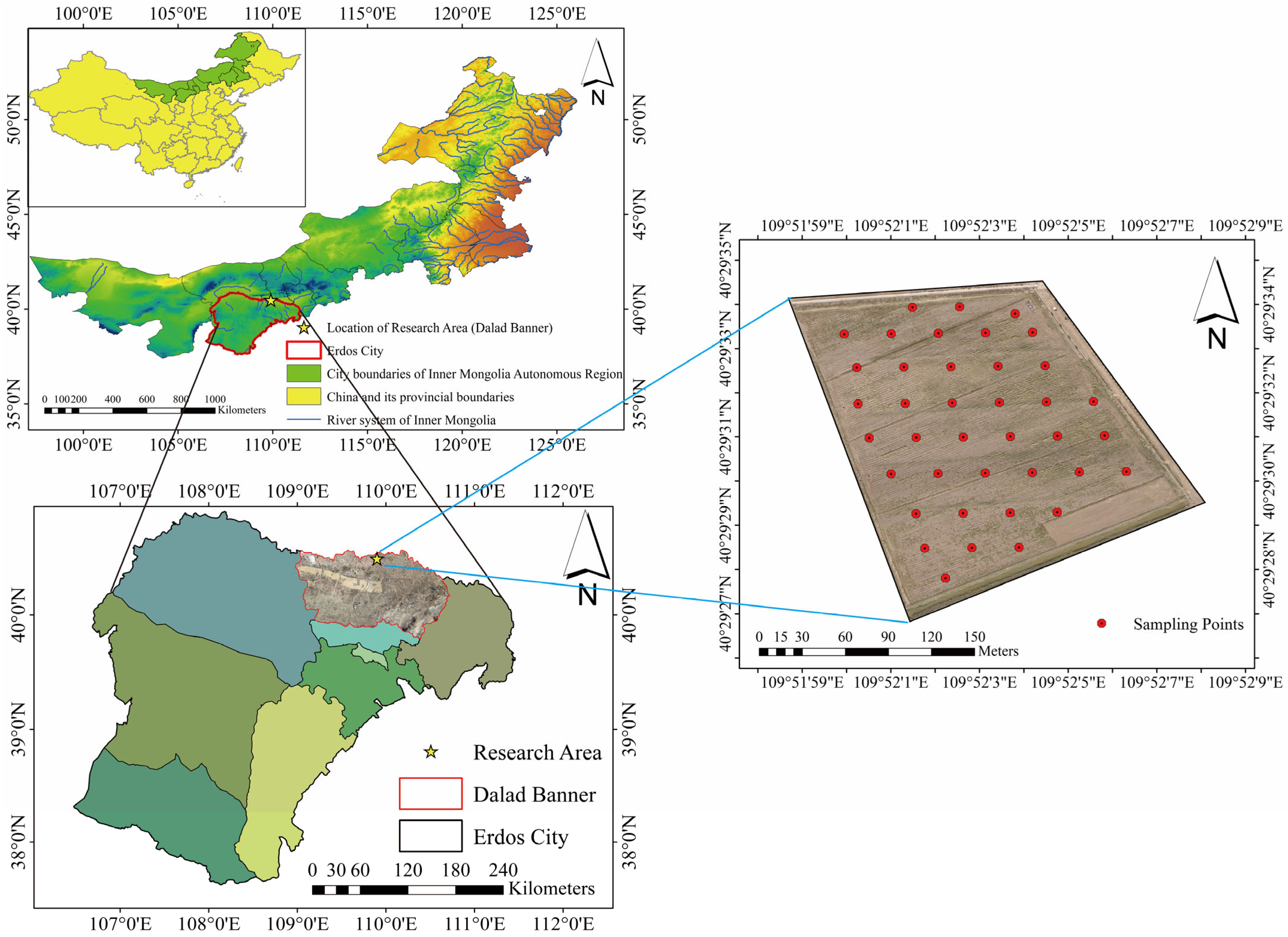
2.1. Study Area

As depicted in Figure 1, our study area encompasses the irrigated region on the Yellow River’s southern banks, encompassing Dalat City in Ordos City, Inner Mongolia Autonomous Region. The geographical coordinates for this area are 106°42′–110°27′ E and 37°35′–40°47′ N. This region experiences an average annual temperature range of 5.9 to 6.3 °C, a frost-free period lasting 158 days, and an average annual precipitation ranging from 281.7 to 301.8 mm. Additionally, the average annual evaporation in this area falls within the range of 2161 to 2600 mm. On 21 July 2022, during surface soil sampling at 39 locations within the study area, soil samples were collected from layers measuring 20–40 mm, 40–60 mm, 60–80 mm, and 80–100 mm. Various physical properties of the soil were assessed (

Table 1. Soil physical properties.

Soil Depth (cm)	Saturation Moisture Content (%)	Field Capacity (%)	Bulk Density (g·cm−3)	Soil Texture
0–20	32.12–35.06	28.69–33.37	1.43–1.46	Silt
20–40	35.77–38.24	31.84–35.67	1.37–1.39	Silt loam
40–60	33.25–38.31	32.01–34.02	1.36–1.40	Silt loam
60–80	27.01–31.85	26.33–29.62	1.43–1.46	Silt loam
80–100	30.45–34.16	28.21–32.34	1.41–1.44	Silt loam

). Utilizing the United States Department of Agriculture (USDA) classification system, the soil was categorized into three particle groups based on size: sand (2–0.02 mm), silt (0.02–0.002 mm), and clay (<0.002 mm). Additionally, 12 texture names were assigned to construct a soil texture triangle. Analysis of the soil texture triangle diagram revealed that the prevailing soil type in this area is silt loam. Because of adverse climatic conditions and imprudent irrigation practices, secondary soil salinization has become a significant issue in this region, with approximately 3.78 × 10⁴ hm² of arable land affected. This situation substantially hampers the prospects of fostering robust and sustainable local agricultural practices. This research chose a 2.67 hm² salinization site as the UAV data collection area within a test region characterized by level terrain and soft soil, with sunflowers as the indicator crop.

2.2. Test Data Acquisition and Processing

2.2.1. Gathering Field Data

The study area, established in 2022 on a recently rehabilitated salinized wasteland, conducted experiments with sunflowers as the designated test crop. Employing the artificial spot planting method [18], the sunflowers were sown on distinct dates, namely, 15 June 2022, and 3 June 2023, with subsequent harvests on 1 October 2022 and 1 October 2023. The employed irrigation techniques involved Yellow River flood irrigation, with supplementary spring and autumn irrigation conducted before planting and after harvest. Notably, no irrigation was administered during the growth period. In this experiment, three growth stages of sunflowers were sampled: budding stage, emerging within 35 to 50 days after emergence; flowering stage, emerging within 50 to 80 days after emergence; and maturity stage, emerging within 80 to 110 days after emergence.

In light of the sunflower’s growth within the test area, soil samples were collected during sunny weather to complement the acquisition of multispectral remote sensing images by UAV. Over two consecutive years, 2022 and 2023, soil samples were gathered from sites suitable for drone photography in the following periods: 20 April 2022 (before spring irrigation), 21 July 2022 (budding stage), 26 August 2022 (flowering stage), 20 September 2022 (maturity stage), 29 April 2023 (before spring irrigation), 15 July 2023 (budding stage), 22 August 2023 (flowering stage), and 27 September 2023 (maturity stage). The coordinates of these sampling points were documented using Ovey maps. Thirty-nine soil sampling points were established (Figure 1). To ensure accuracy, the collection procedure involved the removal of surface withered grass and garbage at the sampling point. A five-point sampling method was applied, centering around the sampling point, and consistently repeated four times, with each repetition approximately two steps away from the central point. Soil samples were obtained from each point at a 0–20 cm depth using a soil sampling drill. Postcollection soil samples underwent a sequence of processes involving natural drying, grinding, and screening. A soil solution was then meticulously prepared with a specific soil–water mass ratio of 1:5. Following thorough mixing and settling, the soil solution’s electrical conductivity (EC, mS cm⁻¹) was assessed using the DDSJ-308F conductivity meter, with 5 repetitions, and the average recorded value represented the soil’s conductivity at the respective sampling point. Ultimately, the SSC was computed using the empirical formula: SSC (g kg⁻¹) = 3.609EC − 0.523.

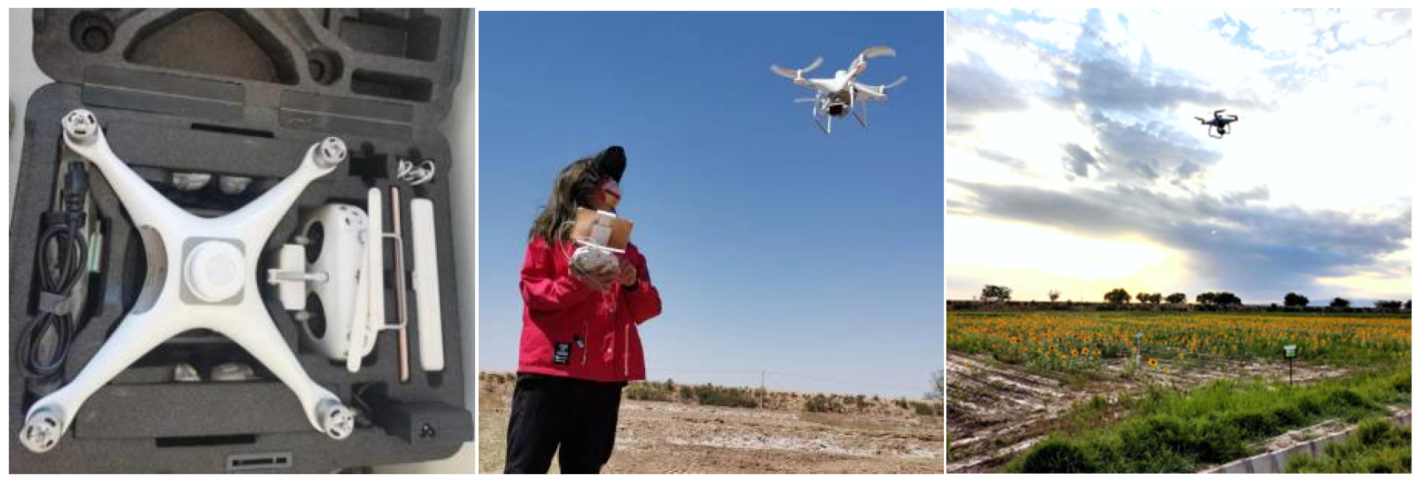
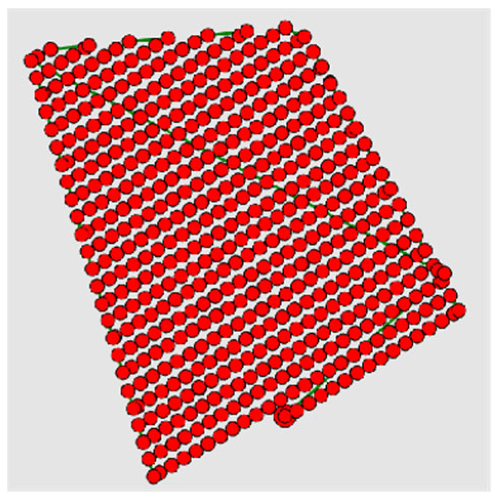
2.2.2. UAV Data Acquisition

The DJI Phantom 4 Multispectral (P4 Multispectral) was employed to capture UAV multispectral images during field sampling period from 11:00 to 14:00 (Figure 2). The P4 Multispectral comprises six 1/29-inch (1 inch ≈ 2.54 cm) CMOS (complementary metal oxide semiconductor) image sensors. Among these sensors, one serves as a color sensor for capturing visible light (RGB) images, while the remaining 5 function as monochrome sensors dedicated to multispectral imaging. The following wavelengths were used: blue (450 nm), green (560 nm), red (650 nm), red edge (RE 730 nm) and near-infrared (NIR 840 nm), with a standard error of 16 nm. The TimeSync system was utilized to achieve microsecond-level synchronous data recording. The flight was conducted at an altitude of 50 m with a speed of 5 m s⁻¹, capturing photos while hovering. The pixel resolution (GSD) was 2.65 cm, and the heading and side overlap degrees were set at 80%. The sensor’s flight path was preconfigured (Figure 3).

The image, comprising five bands and captured through aerial photography, was imported into Pix4D Mapper 4.5.6 software, which is developed by the Swiss company Pix4D. The software automatically combines these bands to generate both a single-band image and an RGB orthophoto image of the UAV. Subsequently, ENVI Classic 5.3 software developed by EVIS Corporation of the United States, was employed for band synthesis and atmospheric correction of the UAV images. The GPS positioning data from the measured sampling points were then imported to obtain the corresponding spectral reflectance values for all five bands.

2.3. Optimization of Spectral Variables

The spectral index is a rapid and noninvasive technique for quantifying the photochemical reflectance index, allowing for the assessment of the surface properties of the observed object [19]. The investigation into the spectral characteristics of saline soil serves as a crucial link in establishing the correlation between ground data and remote sensing data. Given the relatively large standard deviation within the band and the weak correlation between bands, obtaining band combinations through the free integration of spectral reflectance from different bands based on ground characteristics becomes essential. Introducing spectral indicators for the composite calculation of band reflectance is an effective measure for monitoring soil salinization. The introduction of spectral indices has significantly accelerated the growth of the agricultural sector. These indices have been extensively applied to assess various soil types, qualitatively monitor vegetation growth, and model ecological environments [20,21,22]. In this study, a set of representative spectral indices was chosen (

Table 2. Spectral index calculation formula, where B, G, R, RE, NIR, S2, S3, S4, S5, S6, SI1, SI2, SI3, SI, SRSI, BI, Int1, NDVI, VI_opt, DVI, RVI, SI*, SI1*, SI2*, Int1*, Int2*, SI-reg, SI1-reg, SI2-reg, SI3-reg, Int1-reg, and Int2-reg represent the blue band, green band, red band, red edge band, near-infrared band, Salinity index II, Salinity index III, Salinity index IV, Salinity index V, Salinity index Ⅵ, Salinity index 1, Salinity index 2, Salinity index 3, Salinity index, Salinization remote sensing index, Brightness index, Intensity index 1, Normalized difference vegetation index, Optimal vegetation index, Difference vegetation index, Ratio vegetation index, RE-Salinity index*, RE-Salinity index 1*, RE-Salinity index 2*, RE-Salinity index 3*, RE-Intensity index 1*, RE-Intensity index 2*, RE-Salinity index, RE-Salinity index 1, RE-Salinity index 2, RE-Salinity index 3, RE-Intensity index 1, and RE-Intensity index 2, respectively.

Spectral Index	Calculation Formula	Spectral Index	Calculation Formula
S2	S2 = (B − R)/(B + R)	DVI	DVI = NIR − R
S3	S3 = (R × G)/B	RVI	RVI = NIR/R
S4	S4 = (B × R)0.5	SI*	SI* = (RE + R)0.5
S5	S5 = (B × R)/G	SI1*	SI1* = (RE × R)0.5
S6	S6 = (R × NIR)/G	SI2*	SI2* = (G2 + R2 + RE2)0.5
SI1	SI1 = (G × R)0.5	SI3*	SI3* = (RE2 + R2)0.5
SI2	SI2 = (G2 + R2 + NIR2)0.5	Int1*	Int1* = (RE + R)/2
SI3	SI3 = (G2 + R2)0.5	Int2*	Int2* = (G + R + RE)/2
SI	SI = (B + R)0.5	SI-reg	SI-reg = (B + RE)0.5
SRSI	SRSI = ((NDVI − 1)2 + SI12)0.5	SI1-reg	SI1-reg = (G × RE)0.5
BI	BI = (R2 + NIR2)0.5	SI2-reg	SI2-reg= (G2 + RE2 + NIR2)0.5
Int1	Int1 = (G + R)/2	SI3-reg	SI3-reg = (G2 + RE2)0.5
NDVI	NDVI = (NIR − R)/(NIR + R)	Int1-reg	Int1-reg = (G+ RE)/2
VIopt	VIopt = 1.45 × ((NIR2 + 1)/(R + 0.45))	Int2-reg	Int2-reg = (G + RE + NIR)/2

) [23,24,25,26], including 9 salinity indices, the salinization remote sensing index (SRSI), brightness index (BI), intensity index (Int1), 4 planting cover indices, and 12 red-edge spectral indices. Each spectral index’s respective formula was applied within ENVI 5.3 for band calculation. The coordinate position was determined, aligning the measured soil salt points with the spectral index. Subsequently, the spectral variable related to soil salt was enhanced through correlation analysis.

2.4. Model Construction and Accuracy Evaluation

2.4.1. Model Construction

UAV multispectral remote sensing was employed for soil data monitoring for two consecutive years. The soil spectral variables served as the model inputs, while SSC served as the model output. The training and test datasets were randomly partitioned. Because of the rasterization characteristics of the Transformer model, which aim to reduce the computational complexity and enhance prediction accuracy, this study opted for the Transformer to create the SSC inversion model. Additionally, the study utilized a PLSR, BPNN, and RF for training, prediction, and comparison purposes. The entire construction process was carried out using Python 3.8.2.

The PLSR model is a regression modeling method that integrates the strengths of principal component analysis, linear regression analysis, and correlation analysis when handling multiple dependent and independent variables. It effectively solves problems that ordinary multiple regression models cannot address.

The BPNN model is a multilayer feedforward network trained using the error backpropagation algorithm, comprising the input, hidden, and output layers. It is widely recognized as one of the most popular neural network models today.

The RF model is a machine learning method introduced in 1998 that builds an ensemble of unrelated decision trees. It offers robustness to issues like multicollinearity, missing data, and imbalanced samples. As a result, RF is widely utilized as an effective algorithm in machine learning applications.

The Transformer model developed by the Google team in 2017 achieved parallel information input. In contrast to recurrent neural networks (RNNs) that iteratively acquire information and convolutional neural networks (CNNs) limited to local data, the Transformer model directly accesses global information, enabling parallel processing that surpasses the speed of RNNs and enhances data analysis and processing efficiency. The Transformer architecture deviates from traditional CNNs and RNNs, adopting an Attention mechanism with encoding and decoding components and their interconnections. The encoding section comprises a set of encoders, while the decoding section mirrors this setup with an equal number of decoders corresponding to the encoders. The structural layout of the Transformer model is depicted in Figure 4.

2.4.2. Model Accuracy Evaluation

The root mean square error (RMSE), coefficient of determination (R²), mean absolute error (MAE), mean relative error (MRE), and mean deviation error (MBE) were employed to assess and evaluate the model’s stability and predictive accuracy [27,28]. The loss function was utilized to quantify the extent of the model’s performance degradation [29]. The smaller the values of RMSE, MAE, MRE, and MBE, approaching zero, the estimation error decreases, and the precision improves. Similarly, the closer R² is to 1, as the fit improves, the estimation accuracy sees a corresponding increase. The calculation formulas are as follows:

$$RMSE=\sqrt{\frac{{\sum }_i^n{\left({\widehat{y}}_i-y_i\right)}^2}{n}}$$

(1)

$$R^2=1-\frac{{{\sum }_{i=1}^n\left({\widehat{y}}_i-y_i\right)}^2}{{{\sum }_{i=1}^n\left(y_i-{\bar{y}}_i\right)}^2}$$

(2)

$$MAE=\frac{{\sum }_i^n\left|y_i-{\widehat{y}}_i\right|}{n}$$

(3)

$$MRE=\frac{{\sum }_i^n\left|\frac{y_i-{\widehat{y}}_i}{y_i}\right|}{n}$$

(4)

$$MBE=\frac{{\sum }_i^n\left(y_i-{\widehat{y}}_i\right)}{n}$$

(5)

where $y_i$ is the measured value; ${\overline{y}}_i$ is the mean value of the measured value; ${\widehat{y}}_i$ is the model prediction value; and n is the number of samples.

3. Results

3.1. Soil Salinity Characteristics

The surface soil salinity collected at various time intervals is categorized into the following grades: nonsaline soil (<3 g kg⁻¹), light saline soil (3–5 g kg⁻¹), moderately saline soil (5–7 g kg⁻¹), heavy saline soil (7–12 g kg⁻¹), and saline soil (>12 g kg⁻¹); detailed statistical characteristics of the SSC can be found in

Table 3. Statistical analysis of SSC characteristics; Max, Min, Avg., SD, Med., and CV represent the maximum, minimum, average, standard deviation, median, and coefficient of variation, respectively.

Time		Number of Samples						SSC (g/kg)
		Total Sample	Nonsaline Soil	Light Saline Soil	Moderately Saline Soil	Heavy Saline Soil	Saline Soil	Max	Min	Avg.	SD	Med.	CV
2022	Before spring irrigation	40	0	0	0	15	25	32.2	7.0	16.7	7.1	15.8	0.426
	Budding stage	39	0	0	3	7	29	23.1	5.5	14.5	4.7	14.3	0.325
	Flowering stage	39	0	2	2	13	22	24.5	4.0	13.5	5.4	13.4	0.401
	Maturity stage	39	0	3	3	12	21	31.3	4.2	13.9	6.8	13.4	0.492
2023	Before spring irrigation	39	0	1	3	13	22	24.6	4.3	13.9	5.4	14.5	0.389
	Budding stage	39	0	6	8	18	7	15.8	4.0	8.9	3.3	8.7	0.375
	Flowering stage	39	0	10	9	19	1	15.4	4.0	7.4	2.6	7.4	0.355
	Maturity stage	39	1	6	8	19	5	14.3	1.9	8.1	3.1	7.9	0.381

. The study area exhibits a wide range of SSC, with the maximum ranging from 32.2 g kg⁻¹ to 14.3 g kg⁻¹ and the median range falling between 15.8 g kg⁻¹ and 7.4 g kg⁻¹. Based on the classification criteria for soil salinization severity, the study area was categorized as saline soil in 2022. Following the implemented improvements, it will progressively transition into a heavy saline soil region by 2023, aligning closely with findings from field surveys. The coefficient of variation ranges from 0.325 to 0.492, indicating a high degree of dispersion and significant spatial variability in the measured soil data. A total of 313 salt data points were collected during eight sampling occasions, spanning from the Before spring irrigation period in 2022 to the Maturity stage in 2023, and these data were utilized in constructing the model.

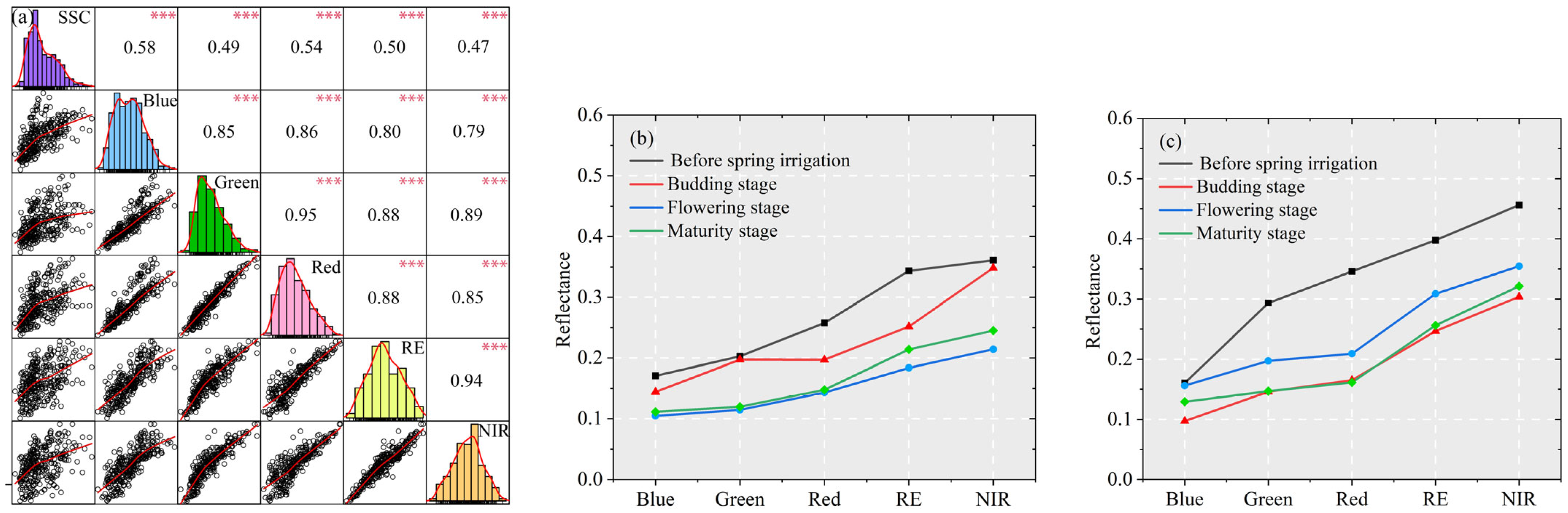
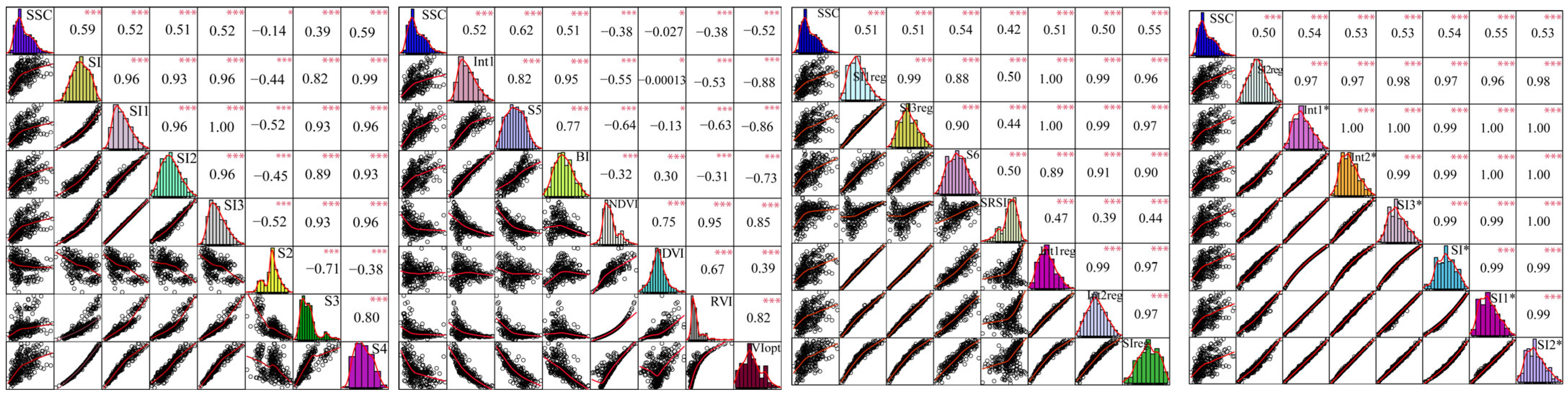
3.2. Correlation between Spectral Variables and SSC

Pearson correlation analysis was performed between 33 spectral variables and the measured surface SSC. The outcomes are displayed in Figure 5 and Figure 6. In Figure 5a, there is a significant correlation at the 0.01 level (p < 0.01) between single-band reflectance and SSC. The Pearson correlation coefficients (PCCs) for the SSC and spectral reflectance in the five bands are as follows: 0.58, 0.49, 0.54, 0.50, and 0.47, respectively. Owing to the heightened energy levels in the blue band, it can stimulate electronic transition within iron oxide, eliciting a distinct optical response. Consequently, the blue band exhibited heightened sensitivity to soil salinity, influenced by the presence of iron oxide in the soil, and its reflectance demonstrates the strongest correlation with soil salinity. The reflectance of each spectral band over two years is illustrated in Figure 5b,c. It is observed that the reflectance before spring irrigation surpasses that during the crop cover stages (including the budding, flowering, and maturity stages). The overall trend in reflectance remains relatively consistent across each period, suggesting that all spectral bands can capture the spectral attributes associated with soil salinity.

In Figure 6, it is evident that the spectral indices strongly associated with SSC include S5, SI, S4, SIreg, SI1*, and S6, with absolute correlation coefficients ranging from 0.54 to 0.62. Among the remaining spectral indicators, except for the negligible correlation between DVI and S2, the absolute correlation coefficients fall within the range of 0.38 to 0.54. The absolute value of the correlation coefficient for red-edge spectral indices, which includes the RE band, ranged from 0.50 to 0.55. This notably enhanced the correlation between UAV remote sensing images and the surface SSC in the demonstration area.

In summary, the input variables for the model, which establish the quantitative relationship between UAV remote sensing images and SSC, were finalized as follows: S5, SI, S4, blue, SIreg, SI1*, red, and S6.

3.3. Construction and Simulation of SSC

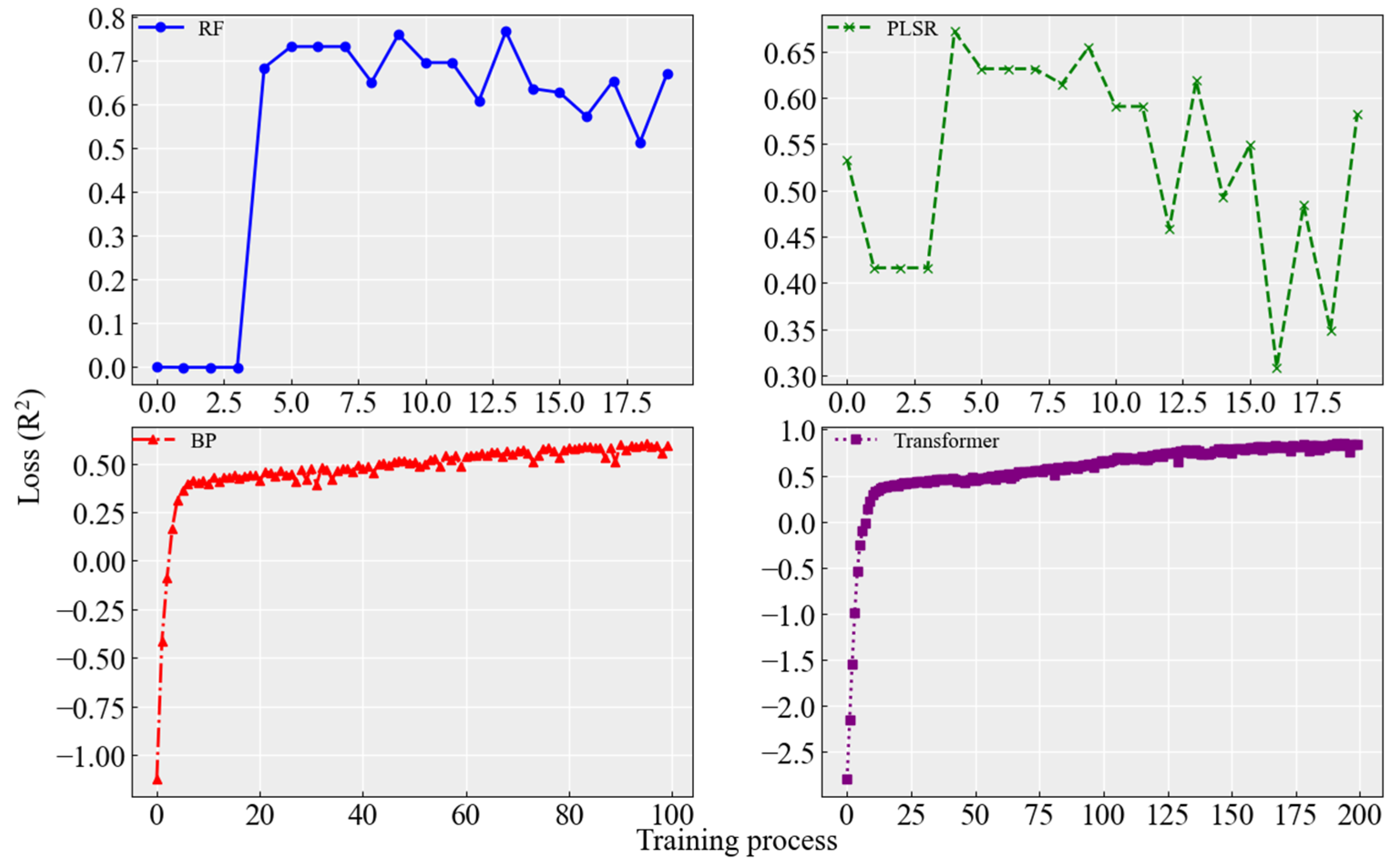
3.3.1. Comparison of the Training Process of Each Model

This study employed three machine learning techniques—RF, PLSR, and BPNN—and deep learning Transformer methods to develop soil salt inversion models. Each model utilized eight spectral variables with strong correlations as input features, and the SSC was generated through simulation transformation. Figure 7 illustrates the line charts depicting the predictions of these four models. As depicted in Figure 7, all four models exhibited a specific capability in SSC inversion. Nevertheless, they tended to underestimate soil samples with a high salt content and overestimate the inversion of individual low-salinity soils, indicating a consistent trend of best-fitting most samples with moderate salinity. Notably, among these models, the Transformer model’s predicted values closely align with the measured values, showcasing the highest level of accuracy.

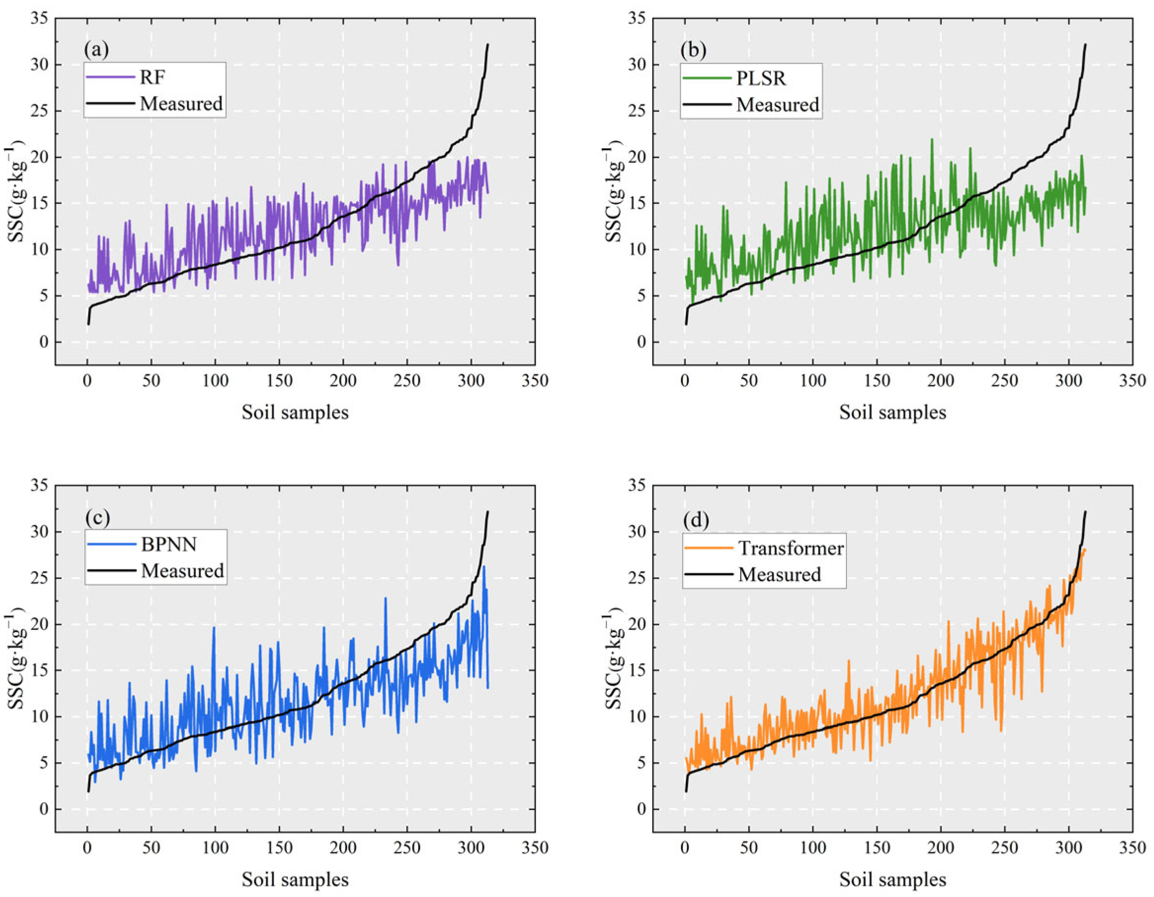
3.3.2. Precision Comparison of Each Model

By comparing the precision evaluation metrics of each model during training (

Table 4. Evaluation index of each model.

Evaluation Index	RF		BPNN		PLSR		Transformer
	Train	Test	Train	Test	Train	Test	Train	Test
RMSE	3.96	3.68	3.98	3.98	4.72	4.10	2.22	2.41
R2	0.56	0.54	0.56	0.46	0.56	0.43	0.83	0.84
MAE	3.04	2.88	3.00	3.08	3.72	3.26	1.67	1.84
MRE	0.29	0.27	0.28	0.30	0.60	0.52	0.17	0.17
MBE	3.04	2.88	3.00	3.08	5.63	5.14	1.67	1.67

), it becomes evident that the Transformer model exhibited the highest prediction accuracy and maintained remarkable stability. The order of RMSE and MAE in the training and test datasets is as follows: Transformer < RF < BPNN < PLSR. While the MRE and MBE were at their lowest in both the training and test datasets for the Transformer model, the PLSR error was the highest. Interestingly, the MRE and MBE for the BP neural network model in the training set were smaller than those for the RF model, which contradicts the comparison results observed in the test set. The R² value for the Transformer model in both the training and test datasets exceeded 0.8, indicating a strong and positive correlation.

The R² was chosen as the evaluation metric for the loss function, and the evolving state of the loss function during the training process of each model was visualized (Figure 8). The model’s stability degree was observed to be in the order of Transformer > BPNN > RF > PLSR. Among these models, the PLSR model exhibited significant fluctuations and the poorest convergence effect. The RF model demonstrated better convergence than the PLSR model but exhibited noticeable fluctuations. In contrast, the BPNN and the Transformer models exhibited faster convergence and reduced fluctuations. However, the Transformer model achieved a significantly superior fitting effect compared to the BPNN model.

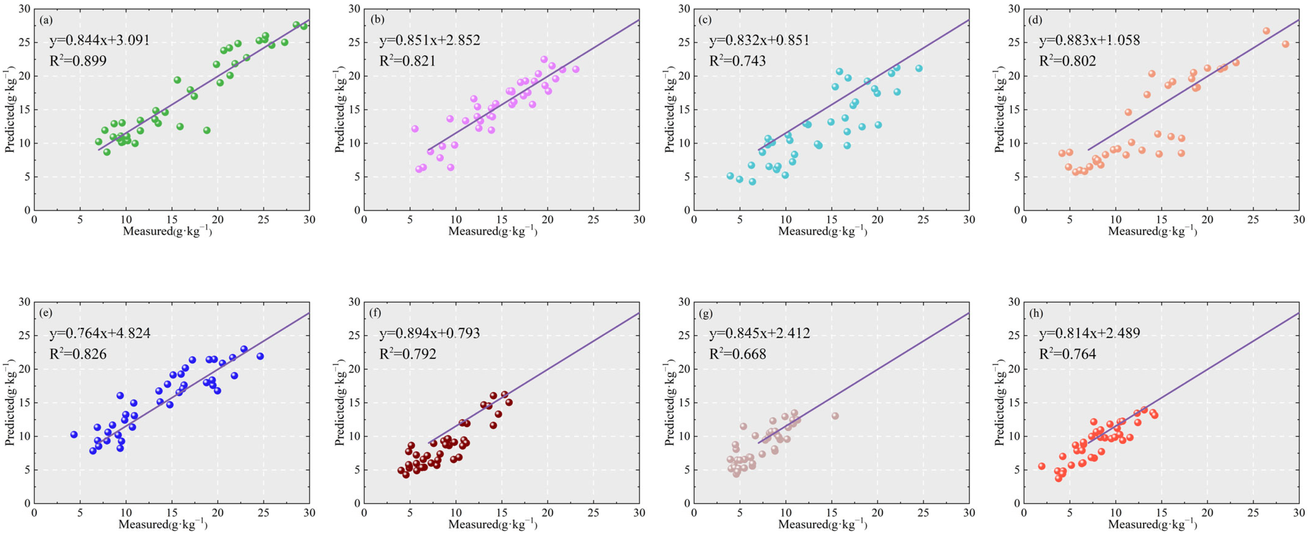
3.3.3. Evaluation of Soil Salinity Accuracy in Different Periods

To investigate the impact of various sampling periods on the Transformer model’s prediction of SSC, the accuracy of SSC was assessed for eight different sampling periods. The Transformer model generated predicted values for the SSC during these periods. The evaluation involved utilizing the R² metric to compare the model’s accuracy further. This analysis is visually represented in Figure 9. Based on the scatter plots presented in Figure 9, it is evident that the model’s accuracy before the spring irrigations in 2022 and 2023 (R² ranging from 0.826 to 0.899) surpassed that during the budding, flowering, and maturity stages (R² ranging from 0.668 to 0.821). This suggests that the inversion effect of the bare soil stage on the SSC outperformed that of the crop cover stage. When comparing the model accuracy across the three crop coverage periods, it was observed that for both years, the order of the accuracy was budding stage > maturity stage > flowering stage. However, the crop coverage degree followed the opposite pattern, with the order being budding stage < maturity stage < flowering stage. This suggests an inverse relationship between crop coverage degree and model accuracy. In other words, as the crop coverage degree increased, the model’s prediction accuracy decreased.

4. Discussion

4.1. RE Band of UAV Remote Sensing Utilized for Soil Salinity Inversion

This study introduced the concept of the RE band. Building upon its strong correlation with the spectral attributes of vegetation canopies and its sensitivity to soil salinity [30], the spectral index was enhanced using the RE band to accomplish soil salinity inversion beneath vegetation cover. During the correlation analysis between single-band reflectance and SSC, it was observed that the absolute correlation coefficient of the red-edge spectral indices, including the RE band, ranged from 0.50 to 0.55. This finding offers robust evidence for enhancing the precision of uncrewed aerial vehicle remote sensing monitoring. The incorporation of RE bands has been shown to enhance the accuracy of soil salinity monitoring, as substantiated by research by numerous scholars. For instance, in multiple studies, Zhao et al. [31,32] utilized input variables, such as the RE band, to model under vegetation cover. They achieved R² values of 0.75 and 0.71, respectively. This reaffirms that multispectral remote sensing of UAVs equipped with the red-edge band can accurately invert the soil salt content under vegetation cover. Cui et al. [33] integrated machine learning, deep learning, and UAV remote sensing to enhance the accuracy of predicting soil salinization during periods of vegetation cover. They employed various vegetation indices, such as NDVI, RVI, and ARVI, including the RE band, to enhance the soil salinity inversion rate under vegetation cover. Three models were developed for comparative analysis. Their findings indicate that the deep learning model using artificial neural networks (ANNs) yielded the most significant improvement in soil salinity inversion, achieving an R² value of 0.79.

4.2. Comparison and Optimization of Soil Salinity Inversion Models

Researchers typically employ a combination of UAV remote sensing and machine learning models to attain precise and efficient regional-scale soil salinity data acquisition. Mukhamediev et al. [34] utilized an optimized spectral index for soil salinity prediction, employing various machine learning algorithms, including XGBoost, LightGBM, RF, support vector machine, and ridge regression. Their findings indicated that the XGB regression model exhibited the most favorable performance, achieving coefficients of determination of up to 0.701. Muratov et al. [35] integrated four machine learning techniques—Gaussian mixture model (GMM), RF, support vector machine (SVM), and K-nearest neighbors (KNN)—with remote sensing technology in their study to enhance the precision of soil salinity monitoring. Wang et al. [36] employed Sentinel-1A synthetic aperture radar (SAR) imagery along with machine learning algorithms, including RFR, multiple linear regression (MLR), and support vector regression (SVR), for investigating variations in soil moisture and salinity. Their analysis revealed that the SVR model exhibited the highest level of accuracy (R² = 0.77) and served as a crucial tool for generating precise and efficient soil–water distribution maps. Thus, this study integrated the PLSR, RF, and BPNN machine learning methods with UAV remote sensing images to investigate salinized soil in the test area. The findings reveal that the BPNN model exhibited the highest stability.

As research deepens, scholars have gradually discovered that while machine learning methods exhibit robust learning and generalization capabilities, they are encumbered by complexities in model structure and calculation processes, a lack of unified criteria for internal function selection and parameter settings, and have challenges in comprehending internal operational mechanisms. Many scholars have proposed improvements to the inversion model to rectify these shortcomings and enhance the predictive precision and stability of soil salinity inversion models. Therefore, enhancing the inversion model has become imperative to rectify this deficiency and enhance soil salinity inversion models’ prediction accuracy and stability. Zhou et al. [37] enhanced the performance of support vector machines through three optimization techniques: gray wolf optimization, particle swarm optimization, and point difference evolution. They then integrated this optimized model with remote sensing technology to enhance the precision of soil salinity prediction in the Aibi Lake region. Lei et al. [38] conducted a comparative analysis involving distributed random forest (DRF), gradient boosting machine (GBM), and deep learning models to investigate the inversion of SSC in sunflower fields. Their findings revealed that the deep learning model attained the highest accuracy level, with R² and normalized root mean square error (NRMSE) values of 0.61 and 0.28, respectively. Hence, this study introduces a deep learning Transformer model to address the limitations of machine learning when integrated with UAV remote sensing technology for soil salt inversion. Furthermore, the accuracy of the soil inversion was compared among the Transformer model, RF model, BPNN model, and PLSR model. The results reveal that the Transformer model exhibited the smallest RMSE, MAE, MRE, and MBE errors for the training and test datasets. Additionally, all determination coefficients, R², exceeded 0.8, indicating the highest model accuracy and a remarkably stable prediction process.

4.3. Accuracy and Reasons of Soil Salinity Inversion Model in Different Growth Stages of Crops

This study yielded positive outcomes in SSC inversion across various periods. Notably, the reflectance before spring irrigation surpasses that during the crop cover stages (budding stage, flowering stage, and maturity stage). This disparity can be attributed to the spring’s freezing and thawing cycle before irrigation, leading to intensified evaporation and subsequent accumulation of soil salts. Consequently, the degree of soil salinization escalates, enhancing spectral reflection [39]. The soil salinization in the study area gradually diminished because of various improvement measures, including sunflower planting during the budding, flowering, and maturity stages, along with irrigation, salt washing, and applying organic fertilizer [40]. Salt-tolerant crops like sunflowers play a vital role in salt absorption from the soil. Through root penetration, they promote soil aeration and drainage, leading to improvements in soil structure and a reduction in soil salinity. Irrigation salt washing involves completely dissolving soil salt into underground water and drainage through concealed pipes. This method aims to reduce the SSC and control groundwater levels. Applying organic fertilizer can enhance soil physical properties, boost soil aggregate formation, alleviate soil compaction, facilitate the migration and decomposition of soil salt, and mitigate salt-related issues in salinized soil. The inversion accuracy of the SSC during the bare soil period surpasses that during the crop cover period due to the absence of ice, snow, and crop cover on the surface [41]. Remote sensing images can more accurately depict surface information during the bare soil period. As the degree of crop cover increases, the model’s predictive accuracy diminishes. Because of the presence of crop cover, shadows can form on the surface, introducing a shadowing effect on optical signals and hindering their complete penetration. Specifically, dense crop cover, like sunflowers, can also lead to multiple scatterings of microwave signals, resulting in a more intricate signal reflection within vegetated regions. This complexity amplifies the challenge of precisely extracting the SSC. Nevertheless, it maintains a robust correlation (R² > 0.668) and effectively mirrors the salinization status in line with field investigations.

Nevertheless, constrained by experimental conditions, this study solely investigated soil salt dynamics during sunflower growth in the field. Further research is warranted to examine soil salt variations under alternative vegetation coverages. Additionally, there needs to be more clarity in sampling depth, data collection timing, and geographical settings within the study area, raising questions about the applicability of these findings to sunflower soil salt inversion in other regions. Validation through future work is imperative.

5. Conclusions

Utilizing multispectral data from UAV, rapid and precise monitoring and inversion of soil salinization in cultivated areas, specifically focusing on a sunflower field within the irrigation zone along the southern banks of China’s Yellow River, were accomplished. This monitoring encompassed the periods before spring irrigation and various crop coverage stages. The soil salinity inversion models were created by integrating multispectral remote sensing data gathered by a UAV, a Transformer deep learning model, and three conventional machine learning techniques. The most effective SSC inversion model was selected based on an evaluation of both the accuracy and stability.

The RE band can enhance the correlation (r > 0.5) between UAV remote-sensing images and soil salinity. The constructed transformer, RF, BPNN, and PLSR models all demonstrated favorable inversion outcomes. Among them, the Transformer model stood out, with the training and test sets’ R² values exceeding 0.8, making it the most stable and accurate prediction model. Comparing the accuracy of the soil salinity at different periods, it Is observed that the inversion effectiveness of the SSC during the bare soil period surpassed that during the crop cover period. Furthermore, an inverse relationship existed between the extent of the crop cover and model accuracy. In summary, using the Transformer deep learning inversion model, in conjunction with the RE band within UAV multispectral data, enhanced the precision of field-scale soil salinity inversion and monitoring within the irrigated region on the southern shores of the Yellow River. This approach offers a scientifically sound management methodology for accurately predicting SSC in the future within the irrigated area of the southern shores of the Yellow River. Additionally, it serves as a valuable reference for utilizing UAV multispectral data.

References

1. Guo, B.; Lu, M.; Fan, Y.; Wu, H.; Yang, Y.; Wang, C. A novel remote sensing monitoring index of salinization based on three-dimensional feature space model and its application in the Yellow River Delta of China. Geomat. Nat. Hazards Risk 2022, 14, 95–116. [Google Scholar] [CrossRef]
2. Li, Y.; Chang, C.; Wang, Z.; Zhao, G. Remote sensing prediction and characteristic analysis of cultivated land salinization in different seasons and multiple soil layers in the coastal area. Int. J. Appl. Earth Obs. Geoinf. 2022, 111, 102838. [Google Scholar] [CrossRef]
3. Rich, V. Chinese irrigation: Yangtze to cross Yellow River. Nature 1983, 305, 568. [Google Scholar] [CrossRef]
4. Gojiya, K.M.; Rank, H.D.; Chauhan, P.M.; Patel, D.V.; Satasiya, R.M.; Prajapati, G.V. Remote Sensing and GIS Applications in Soil Salinity Analysis: A Comprehensive Review. Int. J. Environ. Clim. Chang. 2023, 13, 2149–2161. [Google Scholar] [CrossRef]
5. Gerardo, R.; de Lima, I.P. Sentinel-2 Satellite Imagery-Based Assessment of Soil Salinity in Irrigated Rice Fields in Portugal. Agriculture 2022, 12, 1490. [Google Scholar] [CrossRef]
6. Li, Y.; Chang, C.; Wang, Z.; Zhao, G. Upscaling remote sensing inversion and dynamic monitoring of soil salinization in the Yellow River Delta, China. Ecol. Indic. 2023, 148, 110087. [Google Scholar] [CrossRef]
7. Tronquo, E.; Lievens, H.; Bouchat, J.; Defourny, P.; Baghdadi, N.; Verhoest, N.E.C. Soil Moisture Retrieval Using Multistatic L-Band SAR and Effective Roughness Modeling. Remote Sens. 2022, 14, 1650. [Google Scholar] [CrossRef]
8. Yu, X.; Chang, C.; Song, J.; Zhuge, Y.; Wang, A. Precise Monitoring of Soil Salinity in China’s Yellow River Delta Using UAV-Borne Multispectral Imagery and a Soil Salinity Retrieval Index. Sensors 2022, 22, 546. [Google Scholar] [CrossRef] [PubMed]
9. Bhatt, P.; Maclean, A.L. Comparison of high-resolution NAIP and unmanned aerial vehicle (UAV) imagery for natural vegetation communities classification using machine learning approaches. GIScience Remote Sens. 2023, 60, 2177448. [Google Scholar] [CrossRef]
10. Morcillo, L.; Turrión, D.; Fuentes, D.; Vilagrosa, A. Drone-based assessment of microsite-scale hydrological processes promoted by restoration actions in early post-mining ecological restoration stages. J. Environ. Manag. 2023, 348, 119468. [Google Scholar] [CrossRef] [PubMed]
11. Kariminejad, N.; Kazemi Garajeh, M.; Hosseinalizadeh, M.; Golkar, F.; Pourghasemi, H.R. Harnessing the Power of Remote Sensing and Unmanned Aerial Vehicles: A Comparative Analysis for Soil Loss Estimation on the Loess Plateau. Drones 2023, 7, 659. [Google Scholar] [CrossRef]
12. Wang, J.; Ding, J.; Yu, D.; Ma, X.; Zhang, Z.; Ge, X.; Teng, D.; Li, X.; Liang, J.; Lizaga, I.; et al. Capability of Sentinel-2 MSI data for monitoring and mapping of soil salinity in dry and wet seasons in the Ebinur Lake region, Xinjiang, China. Geoderma 2019, 353, 172–187. [Google Scholar] [CrossRef]
13. Zheng, Q.; Huang, W.; Cui, X.; Shi, Y.; Liu, L. New Spectral Index for Detecting Wheat Yellow Rust Using Sentinel-2 Multispectral Imagery. Sensors 2018, 18, 868. [Google Scholar] [CrossRef] [PubMed]
14. Zhang, Y.; Han, W.; Zhang, H.; Niu, X.; Shao, G. Evaluating soil moisture content under maize coverage using UAV multimodal data by machine learning algorithms. J. Hydrol. 2023, 617, 129086. [Google Scholar] [CrossRef]
15. Shen, F.; Zhao, X.; Kou, G.; Alsaadi, F.E. A new deep learning ensemble credit risk evaluation model with an improved synthetic minority oversampling technique. Appl. Soft Comput. 2021, 98, 106852. [Google Scholar] [CrossRef]
16. Guo, B.; Han, B.; Yang, F.; Fan, Y.; Jiang, L.; Chen, S.; Yang, W.; Gong, R.; Liang, T. Salinization information extraction model based on VI–SI feature space combinations in the Yellow River Delta based on Landsat 8 OLI image. Geomat. Nat. Hazards Risk 2019, 10, 1863–1878. [Google Scholar] [CrossRef]
17. He, Y.; Zhang, Z.; Xiang, R.; Ding, B.; Du, R.; Yin, H.; Chen, Y.; Ba, Y. Monitoring salinity in bare soil based on Sentinel-1/2 image fusion and machine learning. Infrared Phys. Technol. 2023, 131, 104656. [Google Scholar] [CrossRef]
18. Spaeth, M.; Sökefeld, M.; Schwaderer, P.; Gauer, M.E.; Sturm, D.J.; Delatrée, C.C.; Gerhards, R. Smart sprayer a technology for site-specific herbicide application. Crop Prot. 2024, 177, 106564. [Google Scholar] [CrossRef]
19. Ke, Y.; Han, Y.; Cui, L.; Sun, P.; Min, Y.; Wang, Z.; Zhuo, Z.; Zhou, Q.; Yin, X.; Zhou, D. Suaeda salsa spectral index for Suaeda salsa mapping and fractional cover estimation in intertidal wetlands. ISPRS J. Photogramm. Remote Sens. 2024, 207, 104–121. [Google Scholar] [CrossRef]
20. Coelho, A.P.; Faria, R.T.d.; Lemos, L.B.; Rosalen, D.L.; Dalri, A.B. Yield predict and physiological state evaluation of irrigated common bean cultivars with contrasting growth habits by learning algorithms using spectral indices. Geocarto Int. 2022, 37, 15212–15234. [Google Scholar] [CrossRef]
21. Minhoni, R.T.d.A.; Scudiero, E.; Zaccaria, D.; Saad, J.C.C. Multitemporal satellite imagery analysis for soil organic carbon assessment in an agricultural farm in southeastern Brazil. Sci. Total Environ. 2021, 784, 147216. [Google Scholar] [CrossRef]
22. Soltani, I.; Fouad, Y.; Michot, D.; Pichelin, P.; Cudennec, C. Relevance of a near infrared spectral index for assessing tillage and fertilization effects on soil water retention. Soil Tillage Res. 2019, 194, 104345. [Google Scholar] [CrossRef]
23. Reyniers, M.; Walvoort, D.J.J.; De Baardemaaker, J. A linear model to predict with a multi-spectral radiometer the amount of nitrogen in winter wheat. Int. J. Remote Sens. 2007, 27, 4159–4179. [Google Scholar] [CrossRef]
24. Wei, G.; Li, Y.; Zhang, Z.; Chen, Y.; Chen, J.; Yao, Z.; Lao, C.; Chen, H. Estimation of soil salt content by combining UAV-borne multispectral sensor and machine learning algorithms. PeerJ 2020, 8, e9087. [Google Scholar] [CrossRef]
25. Yang, N.; Yang, S.; Cui, W.; Zhang, Z.; Zhang, J.; Chen, J.; Ma, Y.; Lao, C.; Song, Z.; Chen, Y. Effect of spring irrigation on soil salinity monitoring with UAV-borne multispectral sensor. Int. J. Remote Sens. 2021, 42, 8952–8978. [Google Scholar] [CrossRef]
26. Marques, P.; Pádua, L.; Sousa, J.J.; Fernandes-Silva, A. Assessing the Water Status and Leaf Pigment Content of Olive Trees: Evaluating the Potential and Feasibility of Unmanned Aerial Vehicle Multispectral and Thermal Data for Estimation Purposes. Remote Sens. 2023, 15, 4777. [Google Scholar] [CrossRef]
27. Fibbi, L.; Maselli, F.; Pieri, M. Improved estimation of global solar radiation over rugged terrains by the disaggregation of Satellite Applications Facility on Land Surface Analysis data (LSA SAF). Meteorol. Appl. 2020, 27, e1940. [Google Scholar] [CrossRef]
28. Liu, Z.; Wu, Y.; Zhang, X.; Li, M.; Liu, C.; Li, W.; Fu, M.; Qin, S.; Fan, Q.; Luo, H.; et al. Comparison of variable extraction methods using surface field data and its key influencing factors: A case study on aboveground biomass of Pinus densata forest using the original bands and vegetation indices of Landsat 8. Ecol. Indic. 2023, 157, 111307. [Google Scholar] [CrossRef]
29. Garajeh, M.K.; Malakyar, F.; Weng, Q.; Feizizadeh, B.; Blaschke, T.; Lakes, T. An automated deep learning convolutional neural network algorithm applied for soil salinity distribution mapping in Lake Urmia, Iran. Sci. Total Environ. 2021, 778, 146253. [Google Scholar] [CrossRef] [PubMed]
30. Qi, G.; Chang, C.; Yang, W.; Zhao, G. Soil salinity inversion in coastal cotton growing areas: An integration method using satellite-ground spectral fusion and satellite-UAV collaboration. Land Degrad. Dev. 2022, 33, 2289–2302. [Google Scholar] [CrossRef]
31. Zhao, W.; Ma, F.; Yu, H.; Li, Z. Inversion Model of Salt Content in Alfalfa-Covered Soil Based on a Combination of UAV Spectral and Texture Information. Agriculture 2023, 13, 1530. [Google Scholar] [CrossRef]
32. Zhao, W.; Zhou, C.; Zhou, C.; Ma, H.; Wang, Z. Soil Salinity Inversion Model of Oasis in Arid Area Based on UAV Multispectral Remote Sensing. Remote Sens. 2022, 14, 1804. [Google Scholar] [CrossRef]
33. Cui, X.; Han, W.; Dong, Y.; Zhai, X.; Ma, W.; Zhang, L.; Huang, S. Estimating and Mapping Soil Salinity in Multiple Vegetation Cover Periods by Using Unmanned Aerial Vehicle Remote Sensing. Remote Sens. 2023, 15, 4400. [Google Scholar] [CrossRef]
34. Mukhamediev, R.; Amirgaliyev, Y.; Kuchin, Y.; Aubakirov, M.; Terekhov, A.; Merembayev, T.; Yelis, M.; Zaitseva, E.; Levashenko, V.; Popova, Y.; et al. Operational Mapping of Salinization Areas in Agricultural Fields Using Machine Learning Models Based on Low-Altitude Multispectral Images. Drones 2023, 7, 357. [Google Scholar] [CrossRef]
35. Muratov, A.; Omonov, A.; Kato, T.; Fitriyah, A.; Shirokova, Y.; Suvanov, A.; Ismoilov, Z.; Khasanov, S. Integrating spatial database for predicting soil salinity using machine learning methods in Syrdarya Province, Uzbekistan. E3S Web Conf. 2023, 371, 01011. [Google Scholar] [CrossRef]
36. Wang, J.; Wu, F.; Shang, J.; Zhou, Q.; Ahmad, I.; Zhou, G. Saline soil moisture mapping using Sentinel-1A synthetic aperture radar data and machine learning algorithms in humid region of China’s east coast. Catena 2022, 213, 106189. [Google Scholar] [CrossRef]
37. Zhou, X.; Zhang, F.; Liu, C.; Kung, H.-T.; Johnson, V.C. Soil salinity inversion based on novel spectral index. Environ. Earth Sci. 2021, 80, 501. [Google Scholar] [CrossRef]
38. Lei, G.; Zeng, W.; Yu, J.; Huang, J. A comparison of physical-based and machine learning modeling for soil salt dynamics in crop fields. Agric. Water Manag. 2023, 277, 108115. [Google Scholar] [CrossRef]
39. Li, H.; Wang, J.; Liu, H.; Wei, Z.; Miao, H. Quantitative Analysis of Temporal and Spatial Variations of Soil Salinization and Groundwater Depth along the Yellow River Saline–Alkali Land. Sustainability 2022, 14, 6967. [Google Scholar] [CrossRef]
40. Wu, Z.; Li, Y.; Wang, R.; Xu, X.; Ren, D.; Huang, Q.; Xiong, Y.; Huang, G. Evaluation of irrigation water saving and salinity control practices of maize and sunflower in the upper Yellow River basin with an agro-hydrological model based method. Agric. Water Manag. 2023, 278, 108157. [Google Scholar] [CrossRef]
41. Guan, Y.; Grote, K.; Schott, J.; Leverett, K. Prediction of Soil Water Content and Electrical Conductivity Using Random Forest Methods with UAV Multispectral and Ground-Coupled Geophysical Data. Remote Sens. 2022, 14, 1023. [Google Scholar] [CrossRef]
Figure 1. Schematic diagram of the research area and sampling point map.
Agronomy 14 00523 g001
Figure 2. UAV data acquisition process.
Agronomy 14 00523 g002
Figure 3. Route planning and waypoint map.
Agronomy 14 00523 g003
Figure 4. Transformer model structure.
Agronomy 14 00523 g004
Figure 5. (a) PCC between single-band reflectance and SSC, *** indicates a significant correlation at the 0.001 level; (b) reflectance of each spectral band of drone data in 2022; (c) reflectance of each spectral band of drone data in 2023.
Agronomy 14 00523 g005
Figure 6. PCC between spectral index and SSC, *, *** indicates a significant correlation at the 0.05, 0.001 level.
Agronomy 14 00523 g006
Figure 7. Line charts of the prediction models: (a) RF model; (b) PLSR model; (c) BPNN model; (d) Transformer model.
Agronomy 14 00523 g007
Figure 8. Loss changes of each model.
Agronomy 14 00523 g008
Figure 9. Scatterplot of the SSC accuracy for each period: (a) before spring irrigation in 2022; (b) budding stage in 2022; (c) flowering stage in 2022; (d) maturity stage in 2022; (e) before spring irrigation in 2023; (f) budding stage in 2023; (g) flowering stage in 2023; (h) maturity stage in 2023.
Agronomy 14 00523 g009