Modeling of Cotton Yield Estimation Based on Canopy Sun-Induced Chlorophyll Fluorescence

Abstract

Cotton yield estimation is of great practical significance to producers, allowing them to make rational management decisions. At present, crop yield estimation methods mainly comprise traditional agricultural yield estimation methods, which have many shortcomings. As an ideal “probe” for detecting crop photosynthesis, sun-induced chlorophyll fluorescence (SIF) can directly reflect the dynamics of actual crop photosynthesis and has the potential to predict crop yield, in order to realize cotton yield estimation based on canopy SIF. In this study, we set up field trials with different nitrogen fertilizer gradients. The changes of canopy SIF and the physiological parameters of cotton in different growth periods were analyzed. To investigate the effects of LAI and AGB on canopy SIF estimation of cotton yield, four algorithms, Ada Boost (Adaptive Boosting), Bagging (Bootstrap Aggregating), RF (Random Forest), and BPNN (Backpropagation Neural Network), were used to construct cotton yield estimation models based on the SIF and SIFy (the normalization of SIF by incident photosynthetically active radiation) for different time and growth periods. The results include the following: (1) The effects of the leaf area index (LAI) and aboveground biomass (AGB) on cotton canopy SIF and cotton yield were similar. The correlation coefficients of LAI and AGB with cotton yield and SIF were significantly positively correlated with each other starting from the budding period, reaching the maximum at the flowering and boll period, and decreasing at the boll period; (2) In different monitoring time periods, the R² of the cotton yield estimation model established based on SIF and SIFy showed a gradual increase from 10:00 to 14:00 and a gradual decrease from 15:00 to 19:00, while the optimal observation time was from 14:00 to 15:00. The R² increased with the progression of growth from the budding period to the flowering and boll period and decreased at the boll period, while the optimum growth period was the flowering and boll period; (3) Compared to SIF, SIFy has a superior estimation of yield. The best yield estimation model based on the RF algorithm (R² = 0.9612, RMSE = 66.27 kg·ha⁻¹, RPD = 4.264) was found in the canopy SIFy of the flowering and boll period at 14:00–15:00, followed by the model utilizing the Bagging algorithm (R² = 0.8898) and Ada Boost algorithm (R² = 0.8796). In summary, SIFy eliminates the effect of PAR (photosynthetically active radiation) on SIF and can further improve the estimation of SIF production. This study provides empirical support for SIF estimation of cotton yield and methodological and modeling support for the accurate estimation of cotton yield.

1. Introduction

As an important cash crop in the world, cotton is the main raw material for the textile industry and has important uses in the defense, pharmaceutical, and automotive industries [1]. In agricultural production, crop yield forecasting is of great practical importance for producers, allowing them to make rational management decisions, for example, decisions on crop insurance, storage requirements, and cash flow budgets [2]. Cotton’s potential yield can be predicted by physiological parameters such as the leaf area index (LAI) and aboveground biomass (AGB) during crop growth and development [3,4]. Since the application rate of nitrogen fertilizer has a significant effect on both the cotton yield and the physiological parameters [5], predicting the yield is also an important guide for nitrogen application.

Currently, crop yield estimation methods mainly comprise traditional agricultural methods as well as remote sensing technology. Traditional agricultural yield estimation methods require many years of ground data sampling and a large amount of computational processing to build a complete crop yield estimation model; they are time-consuming, involve large survey tasks, high cost, poor timeliness, and other shortcomings, and cannot be instantly applied to a wide range of crop growth monitoring projects [6]. With the rapid development of remote sensing technology in recent years, it has become possible to continuously monitor the growth of agricultural commodities and to extract or estimate crop growth parameters that are closely linked to crop yields, such as the vegetation index, leaf area index, biomass, and productivity [7,8]. This technology has thus become an important tool for crop yield prediction at the regional scale [9,10]. Optical remote sensing, such as hyperspectral techniques, inverts the main biometric and chemical parameters of crops based on spectral profiles and the main parameters of the relevant characteristics, and the reflectance signals characterize the dynamics of the biometric characteristics of the plant [11,12]. Many studies use spectral band reflectance [13], vegetation indices (VIS) [14], the fraction of absorbed photosynthetically active radiation (fAPAR) [15], and lidar-based measurements to estimate crop yield [16]. However, many remote sensing variables have a high correlation with yield, where the prediction accuracy of crop yield cannot fully meet the demand [17,18,19]. Early in the plant’s exposure to external environmental stresses, such as nitrogen stress [20], and before changes in leaf pigmentation and canopy structure occur, the plant is able to adapt to environmental changes by regulating internal physiological mechanisms, such as a decrease in the rate of photosynthesis [21], which leads to an increase in chlorophyll fluorescence and heat dissipation [22]. Therefore, chlorophyll fluorescence, which can directly reveal the internal physiological changes of crops [23], has become a hot research topic in recent years.

Sun-induced chlorophyll fluorescence (SIF) is a spectral signal emitted by the photochemical system of plants between 650 and 800 nm under sunlight conditions [24]. As an ideal “probe” for detecting crop photosynthesis, chlorophyll fluorescence can directly reflect the dynamics of actual crop photosynthesis and is superior to “greenness”-based vegetation indices in crop monitoring [25,26]. A strong linear relationship between crop SIF values and gross primary productivity (GPP) has been observed [27,28,29], with GPP being the main photosynthetic flux directly related to crop yield [30,31]. This relationship therefore provides the basis for a model to estimate crop yield based on SIF [32,33]. In recent years, SIF has offered unique potential for crop yield estimation. Guan et al. [34] presented a framework for estimating hybrid crop yields using SIF and analyzed the correlation between the net primary productivity (NPP) of crop yields and the NPP estimated by SIF. It was found that the yield estimation model using only NIRv data had an accuracy of 64%, while the addition of SIF data increased it to 69% [35].

It has been shown that crop SIF is affected by incident radiation, and since photosynthetically available radiation (PAR) is absorbed by the plants, a small portion of the absorbed radiation is released in the form of SIF; therefore, SIF responds to changes in PAR [36,37,38]. Since SIF photons emitted inside the canopy are reabsorbed by other leaves, which depends not only on the optical properties of the leaf but also on the leaf area index (LAI) and canopy structure, the effect of canopy structure must also be considered when using remotely sensed SIF data to estimate large-scale GPP [39,40]. For example, seasonal variation in the leaf area index (LAI) affects the different peak times of SIF and GPP, which in turn affects the relationship between far-red SIF and GPP [41]. Wang et al. [42] explored the correlation between SIF and aboveground biomass (AGB) to assess the effects of drought on grasslands. Previous studies have also pointed out that the time scale of the observations can change the relationship between the observed SIF and GPP [43]. It has been shown that time averaging can mitigate the noise in SIF observations, leading to a tighter SIF–GPP relationship [44]. However, there is still a lack of direct evidence of noise reduction to improve the relationship between SIF and yield. Most of the current SIF studies are based on the satellite scale, which is highly affected by weather and has a low resolution [45]. It is difficult to accurately assess the performance of SIF in crop yield estimation, and ground-based sensors provide an ideal scale for experimental studies of SIF yield estimation. Therefore, to quantify the use of SIF for yield estimation, it is necessary to explore the effects of radiation and biometric parameters based on ground canopy SIF and establish a mechanistic understanding of their relationship with yield and the effects at different times.

Data optimization and model integration can improve the performance of crop yield estimation models [46]. Machine learning methods are able to utilize empirical data to characterize the relationships between variables, thereby potentially improving the accuracy of the inversion of predictive models. Liu et al. [47] used SIF to predict wheat yield in the Indo-Gangetic Plain and showed that machine learning outperformed two linear regression methods and deep learning methods in predicting wheat yield. Wang et al. [48] used SIF to predict county summer corn yields, and the machine learning algorithm predicted yields with an overall accuracy of 90%. In recent years, various machine learning methods such as Random Forest (RF), Artificial Neural Network (ANN), and Adaptive Boosting (Ada Boost) have been successfully applied to explore the relationship between yields and predictors as they are able to cope with the nonlinear laws between the independent variables and the dependent variable, thus improving the performance of the models [49].

In order to realize cotton yield estimation based on canopy SIF, in this study, we set up field trials with different nitrogen fertilizer gradients. The changes of canopy SIF and the biometric parameters of cotton in different growth periods were analyzed. To investigate the effects of LAI and AGB on canopy SIF estimation of cotton yield, four algorithms, Ada Boost (Adaptive Boosting), Bagging (Bootstrap Aggregating), RF (Random Forest), and BPNN (Backpropagation Neural Network), were used to construct cotton yield estimation models based on the SIF and SIFy (the normalization of SIF by incident photosynthetically active radiation) for different time and growth periods. This study provides methodological and model support for the accurate estimation of cotton yield.

2. Materials and Methods

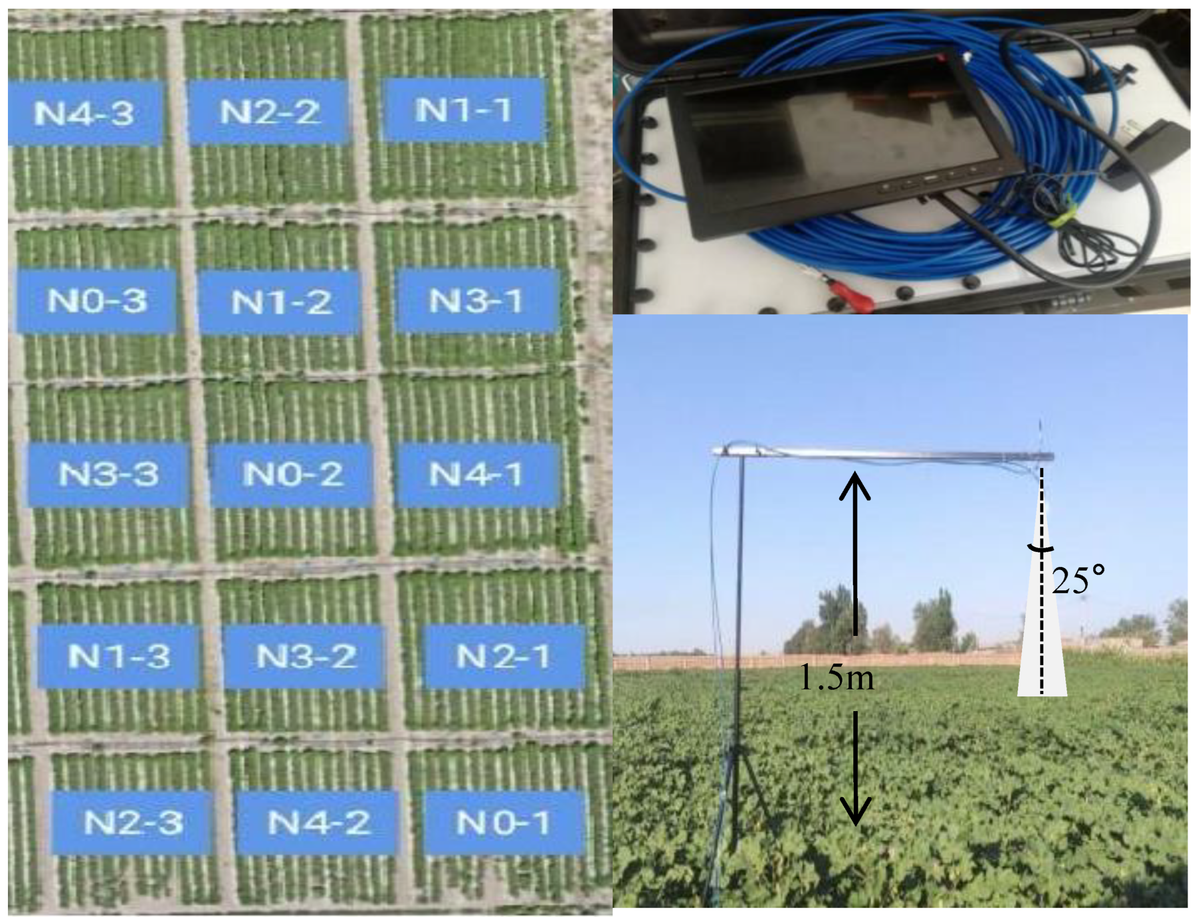
2.1. Overview of the Pilot Area

This study was conducted in Shihezi University Experimental Field, Shihezi City, Xinjiang Uygur Autonomous Region, China (44° 27′ N; 85° 94′ E) from April 2022 to October 2022. The test area is a temperate arid zone climate characterized by abundant light and heat resources. The average annual sunshine hours are 2797.5 h. The annual rainfall is 180–270 mm, and the annual evaporation is 1000–1500 mm. The average annual temperature is 6.6 °C, the highest temperature occurs in July, the average temperature is 24–26 °C, the effective cumulative temperature of ≥10 °C is 3428.5 °C, and the average frost-free period is 176 days. The monthly average temperature and irrigation volume are shown in

Table 1. Climate data for 2023 in the experimental area.

Month	Average High Temperatures	Average Low Temperatures	Total Rainfall
April	18 °C	4 °C	17.2 mm
May	24 °C	12 °C	10.7 mm
June	33 °C	18 °C	36.2 mm
July	35 °C	20 °C	11.7 mm
August	33 °C	18 °C	45.1 mm
September	25 °C	12 °C	25.3 mm
October	20 °C	6 °C	0.1 mm

. The test soil texture in this area was mainly loamy and the basic physicochemical properties were alkaline dissolved nitrogen (ADN) 60.88 mg·kg⁻¹, organic matter (OM) 19.90 mg·kg⁻¹, effective potassium (EK) 134 mg·kg⁻¹, and effective phosphorus (EP) 17.95 mg·kg⁻¹, with the previous crop being cotton. The irrigation quota is the local average, 4050 m³·ha⁻¹, divided into ten irrigation times.

A total of five nitrogen application levels were set up in this study: N0 (0 kg·ha⁻¹), N1 (120 kg·ha⁻¹), N2 (240 kg·ha⁻¹), N3 (360 kg·ha⁻¹), and N4 (480 kg·ha⁻¹). The cell layout is shown in Figure 1. Nitrogen was applied in the form of urea (46% nitrogen content) with water drops, and phosphorus and potash fertilizers (potassium dihydrogen phosphate) were both applied at a rate of 150 kg·ha⁻¹. The application timing of fertilizer was synchronized with the drip application timing of local farmers. The cotton planting date was April 25, 2022, and the tip pruning date was July 13. The planting pattern was “one film, three tubes, and six rows”, and the plant spacing was 10 cm + 66 cm + 10 cm. Each nitrogen treatment plot was replicated three times, with a total of 15 plots and a single plot area of 150 m². A randomized block design was used, with protective rows set around the perimeter, and all other field management measures were carried out according to local high-yield cultivation requirements. Sampling from the budding period occurred every ten days. Three cotton plants with the same growth in each plot were collected each time; there were fifteen plots in total, and the number of plants sampled each time was forty-five.

2.2. Data Acquisition

2.2.1. Canopy Sun-Induced Chlorophyll Fluorescence (SIF) Acquisition

Continuous canopy SIF measurements were collected using the Auto SIF (Bergsun Inc., Beijing, China) field spectroscopy system [50]. Basic parameters of Auto SIF are shown in

Table 2. Basic parameters of Auto SIF.

Parameters	Presentation
Spectral range	640–800 nm, HR 200–1000 nm
Spectral resolution	0.39 nm, HR 1 nm
Spectral response	Up to 70% quantum efficiency at 780 nm, up to 50% quantum efficiency at 680 nm
Optical transmission mode	Bifurcated fibers, prisms, multi-channel MPM
Temperature control system	Temperature range 25 ± 1.00 °C, humidity level < 60% (except under extreme conditions)
Fiber optics	600 µm, 1000 µm

. The sensor probe was placed vertically downward at a vertical height of approximately 1.5 m from the top of the cotton leaves (Figure 1), and the measurement time was from 10:00 to 19:00 (local solar time) with a time sampling interval of 4–7 min. The instrument used the three-band Fraunhofer line depth (3FLD) fluorescence extraction algorithm to extract the SIF value of vegetation [51], and the SIF value of each time period represented the SIF value of the time period on average.

2.2.2. Cotton Biometric Parameters and Yield Data Acquisition

Experimental data collection and measurements were taken at ten-day intervals starting from the budding period for a total of seven collections. Three cotton plants with uniform growth were collected as samples from each plot. The following biometric parameters were measured:

• Leaf area index (LAI): The leaf area data were obtained by using an LI-3100c bench leaf area instrument (LI-COR, Inc., Lincoln, NE, USA) to measure the leaf area of all the leaves of each cotton plant. The formula for calculating LAI is as follows: m is the number of plants measured; A is the leaf area of all leaves of plant m; p is the planting density;

$$\mathrm{L}\mathrm{A}\mathrm{I}=0.75 \rho \frac{{\sum }_{\mathrm{i}=1}^{\mathrm{m}}\mathrm{A}}{\mathrm{m}}$$

(1)

2.

Aboveground biomass (AGB) (g·m⁻²): Once the measured plants were collected, the plants at the upper part of the cotyledon node were cut into pieces and packed in bags. The plants were defoliated at 105 °C for 30 min and dried at 80 °C to a constant weight. AGB is calculated by the following formula: B is the dry weight of a cotton plant and S is the area occupied by a cotton plant;

$$\mathrm{A}\mathrm{G}\mathrm{B}=\frac{\mathrm{B}}{\mathrm{S}}$$

(2)

3.

Seed cotton yield (kg·ha⁻¹): Yield estimation using sample method harvesting. During the cotton fluffing period, representative sample squares (2.28 m × 1 m) were selected from each plot for yield determination; the number of plants, number of bolls per plant, and single boll weight were determined, and the weight of seed cotton was weighed in each sample square. The formula is as follows:

Seed cotton yield (kg·ha⁻¹) = Harvest density (number of plants·ha⁻¹) × Number of bolls per plant (number of individuals·plants⁻¹⁾ × Single boll weight (g)/1000 × Measurement yield correction factor (90%)

(3)

2.3. Data Processing

2.3.1. SIF Data Preprocessing

The determination of the instantaneous intensity of SIF throughout the day using the sun-induced chlorophyll fluorescence (Auto SIF) is susceptible to the influence of the intensity of the effective solar radiation. Normalization of SIF by PAR can reduce the impact of incident radiation intensity on canopy SIF intensity, and improve the effectiveness and accuracy of SIF spectrum detection of crop biometric information [52].

$$\mathrm{P}\mathrm{A}\mathrm{R}={\int }_{\mathsf{\lambda }=400}^{\mathsf{\lambda }=700}{\mathrm{I}}_{\mathsf{\lambda }}\mathrm{d}\mathsf{\lambda }$$

(4)

$$\mathrm{S}\mathrm{I}\mathrm{F}\mathrm{y}=\frac{\mathrm{S}\mathrm{I}\mathrm{F}}{\mathrm{P}\mathrm{A}\mathrm{R}}$$

(5)

2.3.2. Correlation Analysis

All 45 sets of data collected in each period were used for the application of Pearson correlation analysis. The correlation coefficient is an indicator of the closeness of the correlation between the corresponding variables. It is derived by the product-difference method, which is based on the deviation of two variables from their respective mean values, and the degree of correlation between the two variables is reflected by multiplying the two deviations. The formula for calculating the correlation coefficient is as follows: x_i and y_i denote the ith corresponding value of the two parameters, $\overline{\mathrm{x}}$ and $\overline{\mathrm{y}}$ denote the mean value of the two parameters, and n is the number of samples. The higher the value of the correlation coefficient of the samples, the higher the degree of similarity, and vice versa, the lower the degree of similarity.

$$\mathrm{r}=\frac{\sum _{\mathrm{i}=1}^{\mathrm{n}}({\mathrm{x}}_{\mathrm{i}}-\overline{\mathrm{x}})({\mathrm{y}}_{\mathrm{i}}-\overline{\mathrm{y}})}{\sqrt{\sum _{\mathrm{i}=1}^{\mathrm{n}}{({\mathrm{x}}_{\mathrm{i}}-\overline{\mathrm{x}})}^2}\sqrt{\sum _{\mathrm{i}=1}^{\mathrm{n}}{({\mathrm{y}}_{\mathrm{i}}-\overline{\mathrm{y}})}^2}}$$

(6)

2.3.3. Model Building Methodology

The Ada Boost (Adaptive Boosting) algorithm, proposed by Freund et al., in 1996 [53], is an ensemble learning technique that constructs a robust classifier by combining multiple weak classifiers to achieve higher accuracy and mitigate the risk of overfitting. One notable advantage of Ada Boost lies in its adaptive selection of iteration coefficients, which enhances convenience and usability. Moreover, this algorithm serves as a versatile framework for integrating various other algorithms, making it widely adopted in practice.

Bagging (Bootstrap Aggregating) is an integrated learning algorithm commonly used to reduce the variance of predictive models [54]. In the Bagging method, a random sample of data is selected from the training set using the substitution method, allowing for multiple selections of a single data point. Subsequently, these weak models are individually trained and their predictions are aggregated to yield more accurate estimates based on the task type (e.g., regression or classification). Bagging integrates ridge algorithms to improve their accuracy and stability while reducing the variance of the results and avoiding overfitting.

RF (Random Forest) is to build a forest in a random way, and the forest is composed of many decision trees, and each decision tree in the Random Forest is not related to each other. After obtaining the forest, when a new input sample comes in, let each decision tree in the forest make a judgment to see which category the sample should belong to. Then, see which category is selected the most, and predict this sample to be that category. By sampling data sets, multiple different data sets are generated, and a classification tree is trained on each data set. Finally, the prediction results of each classification tree are combined as the prediction results of Random Forest. Random Forest improves the prediction accuracy without a significant increase in computation [55].

BPNN (Backpropagation Neural Network) can learn and store a large number of input–output mode mapping relationships without revealing the mathematical equations describing those relationships. The calculation process consists of a forward calculation process and a reverse calculation process. The forward propagation process is where the input pattern is processed layer by layer from the input layer to the hidden unit layer and shifted to the output layer, where the state of the neurons in each layer only affects the state of the neurons in the next layer. If the desired output cannot be obtained at the output layer, it is transferred to backpropagation, which returns the error signal along the original connection pathway and minimizes the error signal by modifying the weights of each neuron [56].

In this study, the above algorithms are implemented using a machine learning library in the Python language, and the entire data set is randomly divided into a training set and a test set in a ratio of 2:1 to fit the four algorithms.

2.3.4. Evaluation of the Model

The present study employed coefficient of determination (R²), root mean square error (RMSE), and relative percentage difference (RPD) as evaluation metrics. R² is utilized to assess the correlation between the predicted and actual values of a sample. The closer R² is to 1, the stronger the correlation between these two values. The RMSE value is expressed in the same unit as the original observation. The RMSE can quantify the average magnitude of prediction errors produced by the model, and a smaller value indicates a closer match between the predicted values and actual observations, thus indicating a better fit of the model. The RPD is employed to assess the stability performance of the model. A higher RPD indicates a superior stability performance, typically with an RPD value greater than 3 being suitable for practical applications. The specific calculation is determined by the following formula: x_i is the simulated value, y_i is the actual value, n is the number of samples available for validation, and SD is the standard deviation.

$${\mathrm{R}}^2=1-\frac{\sum _{\mathrm{i}=1}^{\mathrm{n}}{({\mathrm{x}}_{\mathrm{i}}-{\overline{\mathrm{y}}}_{\mathrm{i}})}^2}{\sum _{\mathrm{i}=1}^{\mathrm{n}}{({\mathrm{y}}_{\mathrm{i}}-{\overline{\mathrm{y}}}_{\mathrm{i}})}^2}$$

(7)

$$\mathrm{R}\mathrm{M}\mathrm{S}\mathrm{E}=\sqrt{\frac{\sum _{\mathrm{i}=1}^{\mathrm{n}}{({\mathrm{x}}_{\mathrm{i}}-{\mathrm{y}}_{\mathrm{i}})}^2}{\mathrm{n}}}$$

(8)

$$\mathrm{R}\mathrm{P}\mathrm{D}=\mathrm{S}\mathrm{D}/\mathrm{R}\mathrm{M}\mathrm{S}\mathrm{E}$$

(9)

3. Results

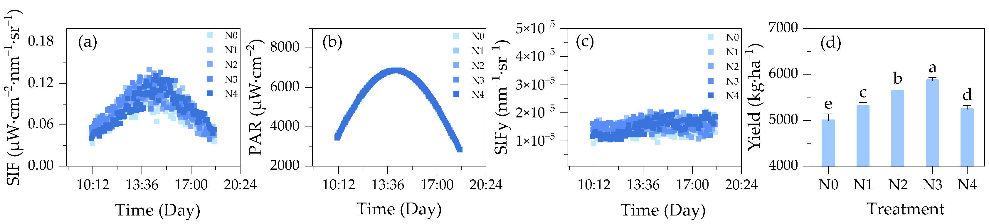
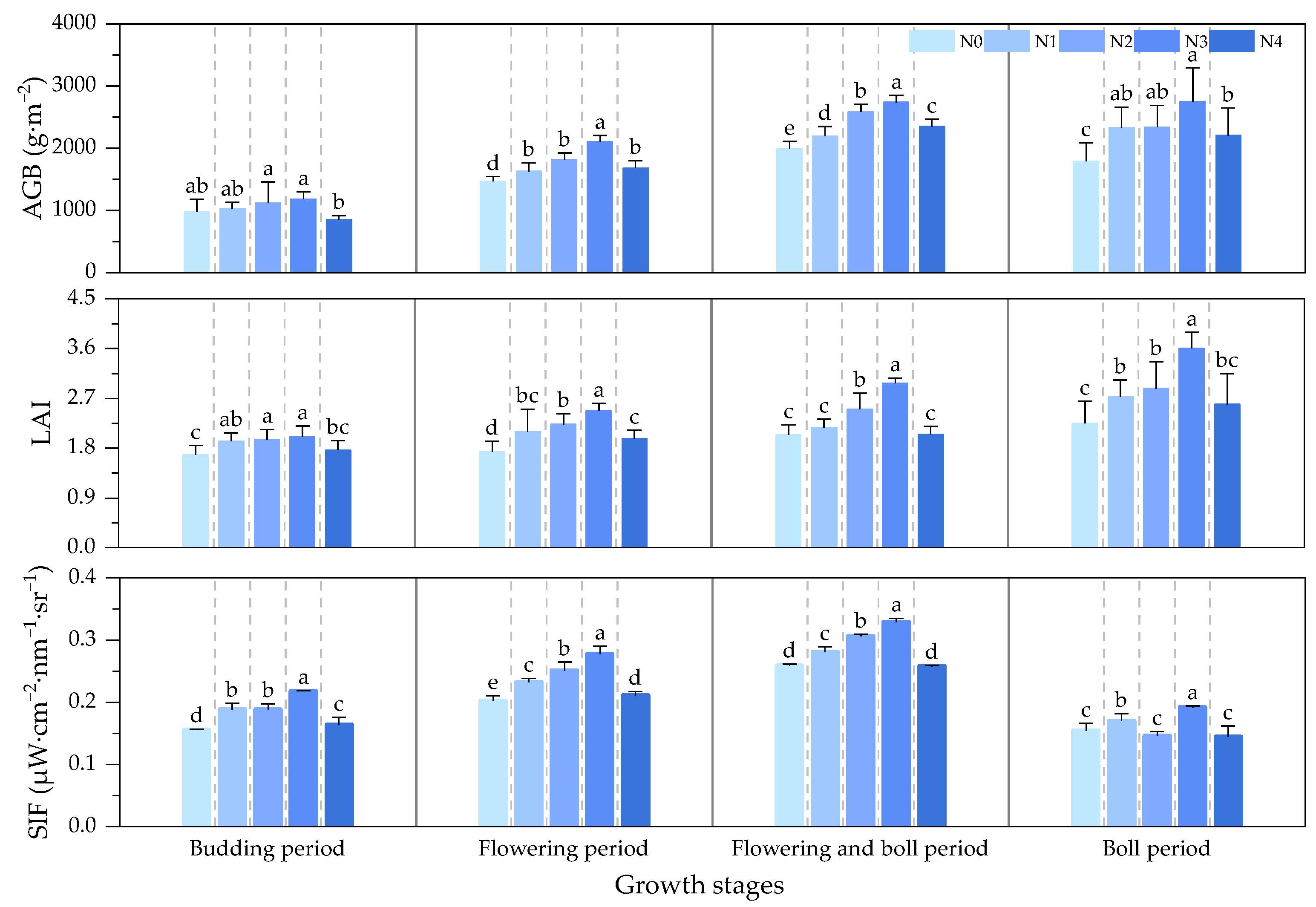
3.1. Diurnal Variation in Canopy SIF and Biometric Parameter Responses of Cotton for Different Growth Periods

The analysis showed that the fluctuation of diurnal variation in cotton canopy SIF showed a single-peak state of first rising and then decreasing on sunny days (Figure 2a), and reached the maximum value around 14:00–15:00. The diurnal variation trends of photosynthetically active radiation (PAR) and SIF were consistent, indicating that PAR affected the change in SIF, and the peak value appeared around 14:00–15:00 (Figure 2b). The diurnal variation in SIFy showed a horizontal linear fluctuation (Figure 2c). Cotton yield showed a trend of first increasing and then decreasing under different nitrogen application treatments, reaching the maximum value under N3 treatment, and the differences among different treatments reached significant levels (Figure 2d).

The variation trends of cotton AGB and LAI during the growing period were basically the same, increasing from the budding period, reaching the maximum value in the flowering and boll period, and decreasing during the boll period (Figure 3). At each growth period, cotton AGB and LAI showed a trend of first increasing and then decreasing with the increase in nitrogen application, and reached the maximum value under the N3 treatment. Cotton canopy SIF increased from the budding period, reached the maximum value at the flowering and boll period, and began to decrease at the boll period (Figure 3). With the increase in nitrogen application, cotton canopy SIF showed a trend of first increasing and then decreasing, and reached the maximum value under the N3 treatment. The change trend of SIF was basically consistent with that of AGB and LAI. These results indicated that AGB and LAI influenced the changes of SIF during the growth period of cotton.

3.2. Correlation Analysis between Canopy SIF and Cotton Yield at Different Growth Periods

3.2.1. Correlation Analysis of Cotton Yield with AGB and LAI at Different Growth Periods

The correlation between cotton yield and biometric parameters was analyzed, and the results are shown in

Table 3. Correlation analysis of cotton yield with AGB and LAI in different growth periods.

	Budding Period	Flowering Period	Flowering and Boll Period	Boll Period
Yield and AGB	0.420 *	0.858 **	0.868 **	0.556 **
Yield and LAI	0.494 *	0.691 **	0.819 **	0.690 **

*, significant correlation at the 0.01 level; **, significant correlation at the 0.05 level.

. In the four key growth periods, cotton yield was significantly positively correlated with AGB and LAI. The correlation coefficient increased first and then decreased with the progress of growth periods and reached the maximum value during the flowering and boll period. The correlation coefficient between yield and AGB reached the maximum value of 0.868 during the flowering and boll period, followed by 0.858 in the flowering period and 0.556 in the boll period. In these three periods, there were significant correlations at the p < 0.05 level. The correlation coefficient between yield and LAI reached the maximum value of 0.819 in the flowering and boll period, followed by 0.691 in the flowering period, while the lowest value was observed during the budding period. The results showed that cotton yield was significantly correlated with both AGB and LAI from the flowering period to the boll period.

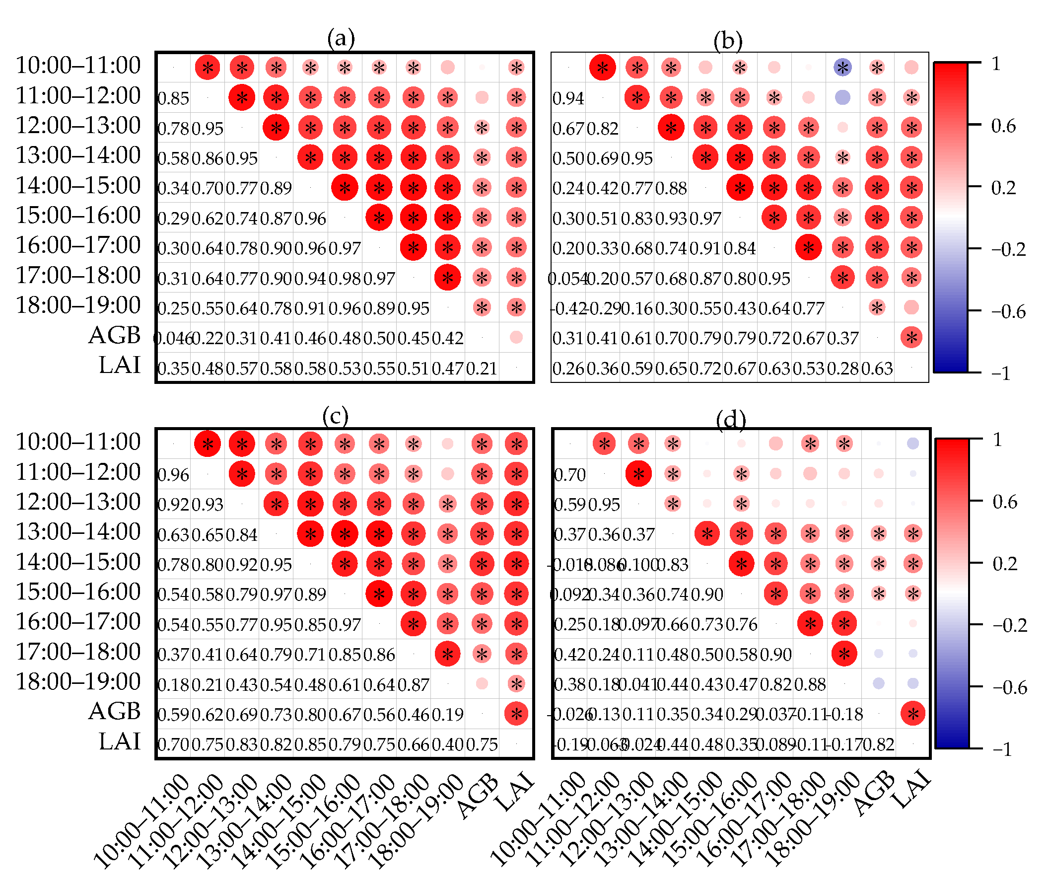
3.2.2. Correlation Analysis of Cotton Canopy SIF with AGB and LAI at Different Growth Periods

As can be seen from Figure 4, the correlation between cotton canopy SIF, AGB, and LAI was the best in the flowering and boll period, followed by the flowering period and the budding period, and it was the smallest during the boll period. In terms of the correlation between cotton canopy SIF and AGB, the correlation first increased and then decreased with the increase in time. The correlation coefficient between SIF and AGB reached the maximum value (r = 0.80) at 14:00–15:00 in the flowering and boll period, followed by that in the flowering period (r = 0.79). In terms of the correlation between cotton canopy SIF and LAI, the correlation first increased and then decreased with the increase in time. The correlation coefficient between SIF and AGB reached the maximum value (r = 0.85) at 14:00–15:00 in the flowering and boll period, followed by that in the flowering period (r = 0.71). The results showed that canopy SIF was significantly correlated with AGB and LAI during the four key reproductive periods, with the highest correlation at 14:00–15:00.

3.3. Construction of the Cotton Yield Estimation Model

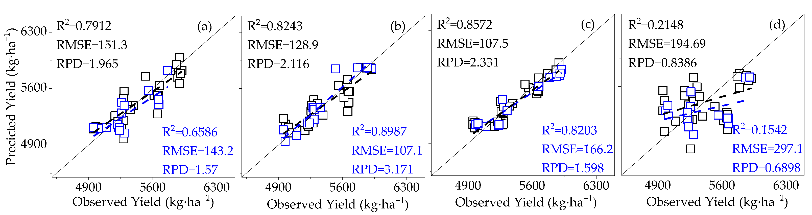
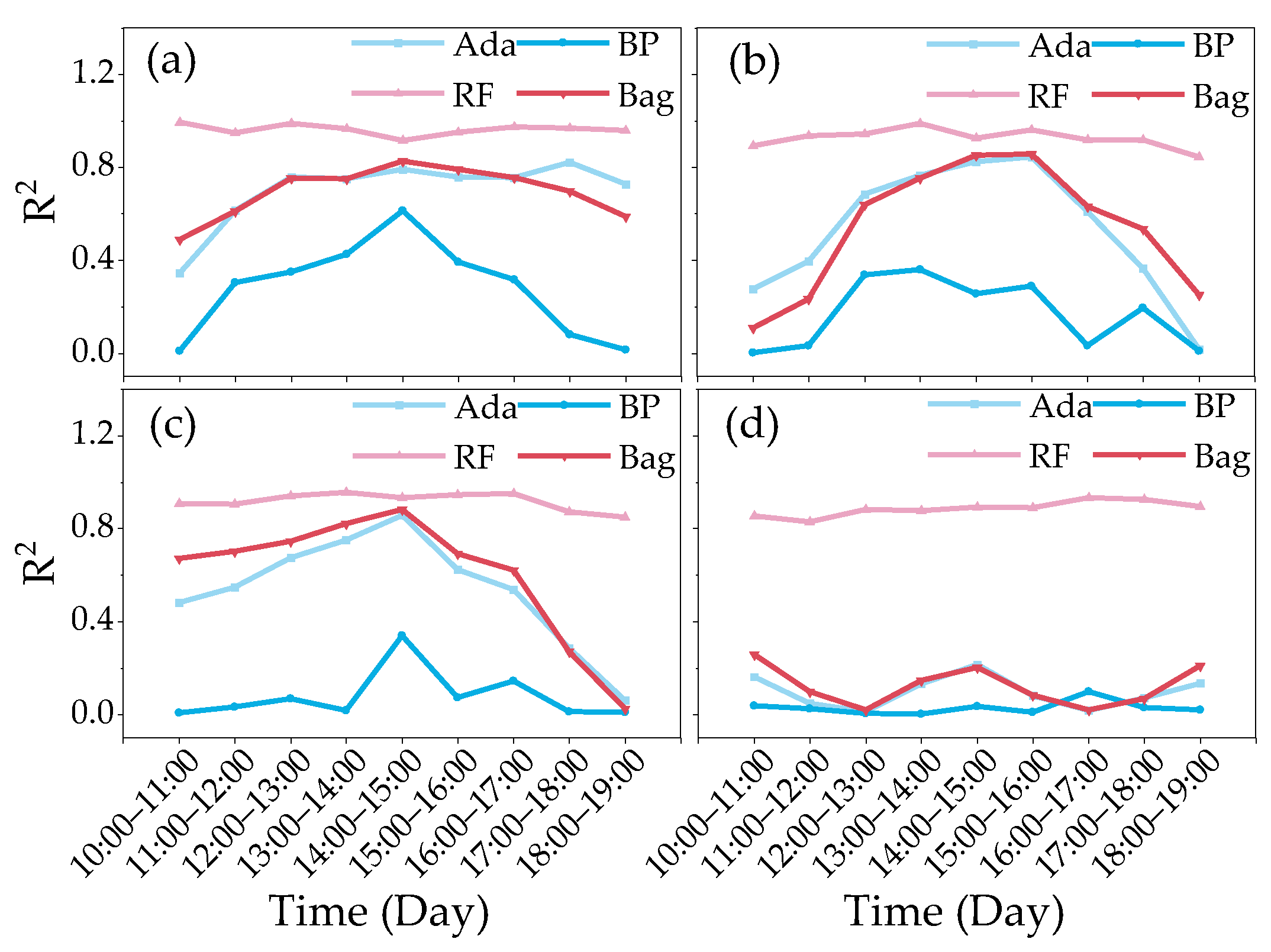
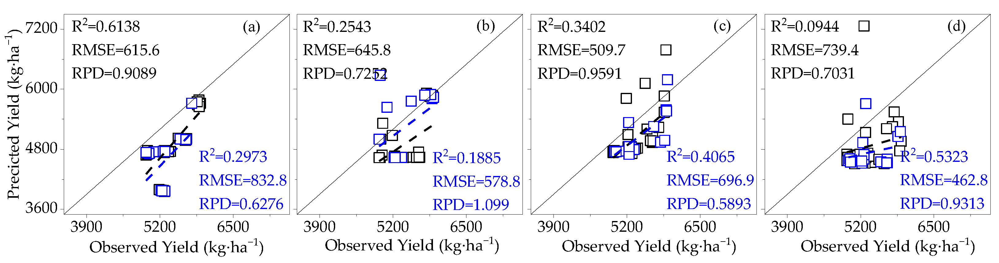
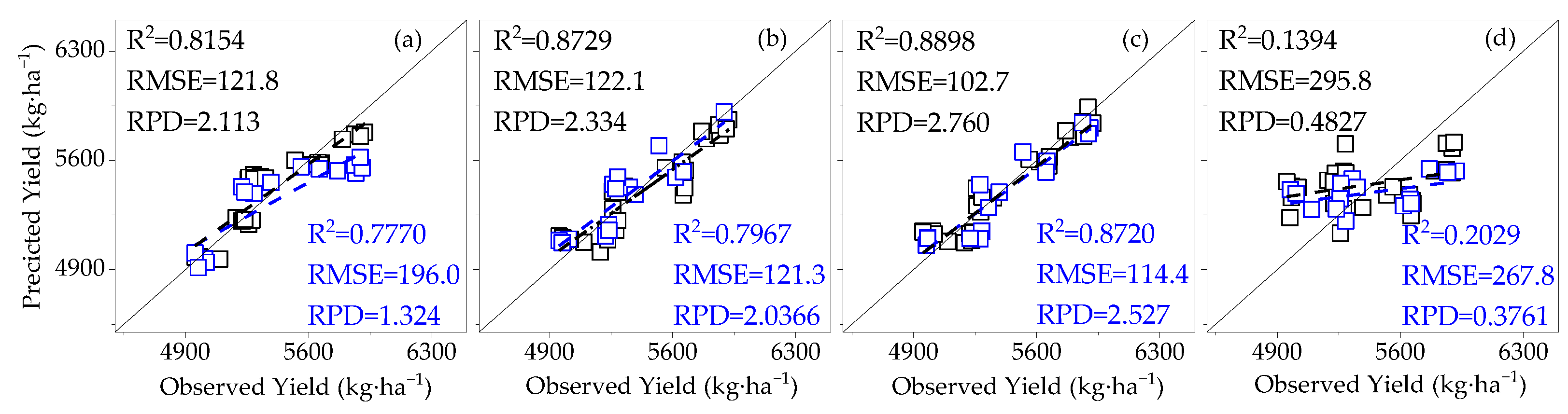
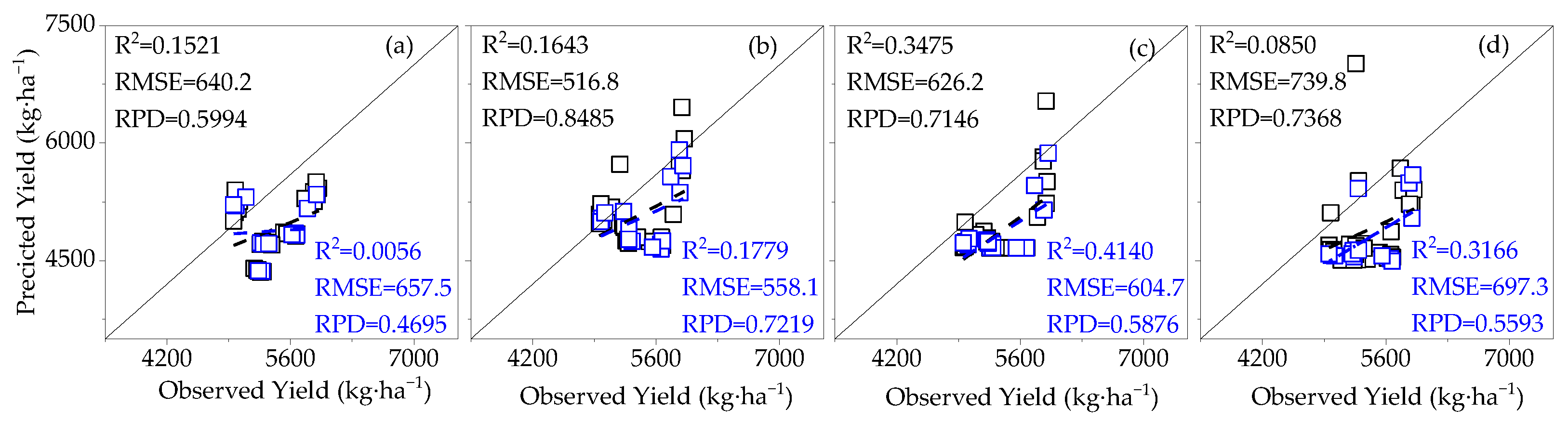
3.3.1. Construction of the Cotton Yield Estimation Model Based on Canopy SIF

The variation in canopy SIF with respect to the cotton yield estimation model R² is shown in Figure 5. In the four key growth periods, the effect of the cotton yield model constructed with RF is the best, and the R² is basically 0.90 in each period. The R² of the cotton yield model constructed using Ada Boost and Bagging had a significant peak at 14:00–15:00, and the range of R² was 0.70–0.80. The model of cotton yield based on BPNN had the worst effect, with R² less than 0.5. In the flowering and boll period (Figure 5c), the constructed models gave better results for all models except BPNN. In the boll period (Figure 5d), none of the models worked very well. This indicates that time variation had an effect on the SIF cotton yield model.

According to the correlation analysis between LAI, AGB, and canopy SIF, canopy SIF with good correlation on 14:00–15:00 was selected. A cotton yield estimation model based on canopy SIF from 14:00 to 15:00 was established. Figure 6, Figure 7, Figure 8 and Figure 9 show the yield estimation model of canopy SIF based on 14:00–15:00 at different growth stages of cotton. By comparing the four modeling methods, it was concluded that the cotton yield model constructed with RF had the best effect (Figure 7). The best modeling using the RF algorithm was achieved during the flowering and boll period (R² = 0.9336, RMSE = 75.16 kg·ha⁻¹, RPD = 3.668, Figure 7c), followed by the flowering period (R² = 0.9256, Figure 7b), while the worst modeling was achieved during the boll period (R² = 0.8919, Figure 7d). The results of utilizing the BPNN algorithm were unsatisfactory for all growth periods, with a maximum R² value of 0.6138 (Figure 9a). The Ada Boost algorithm was used to achieve the best modeling effect in the flowering and boll period (R² = 0.8572, RMSE = 107.5 kg·ha⁻¹, RPD = 2.331, Figure 6c). The Bagging algorithm was able to achieve the best modeling effect in the flowering and boll period (R² = 0.8830, RMSE = 119.7 kg·ha⁻¹, RPD = 2.236, Figure 8c). In summary, the best modeling was achieved for the flowering and boll period, followed by the flowering period, in the yield estimation model based on 14:00–15:00 canopy SIF. The optimal model was RF modeling in the boll period.

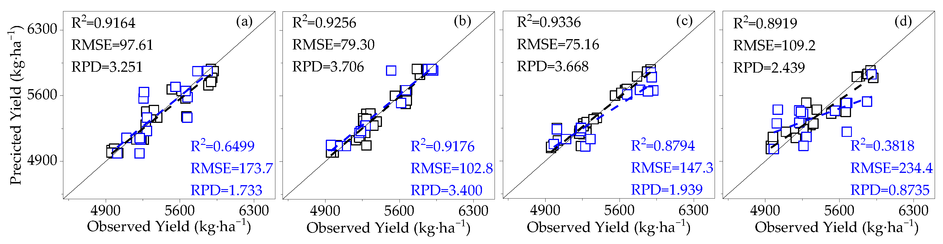
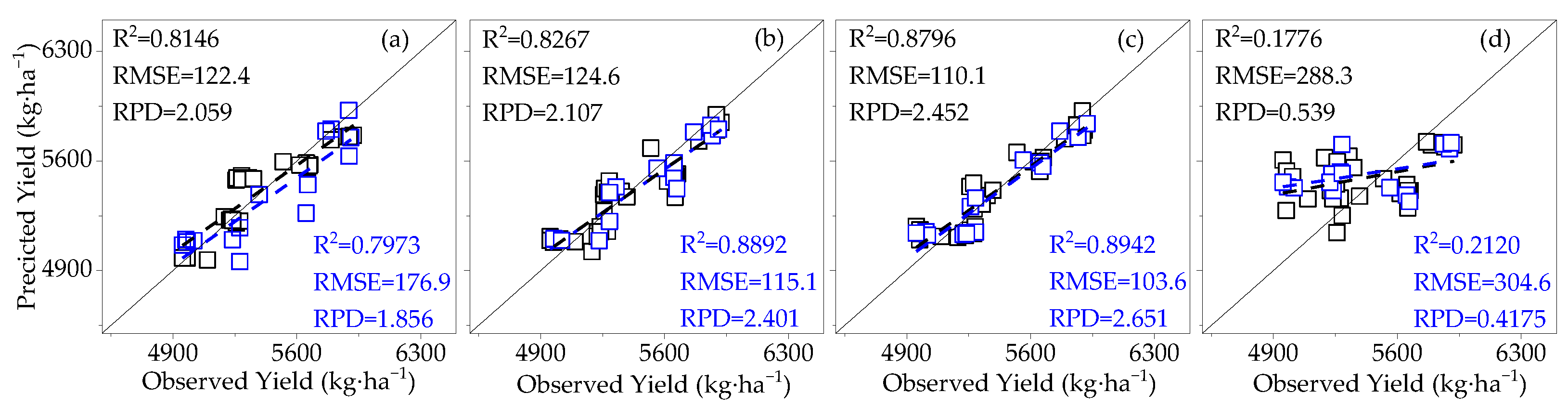
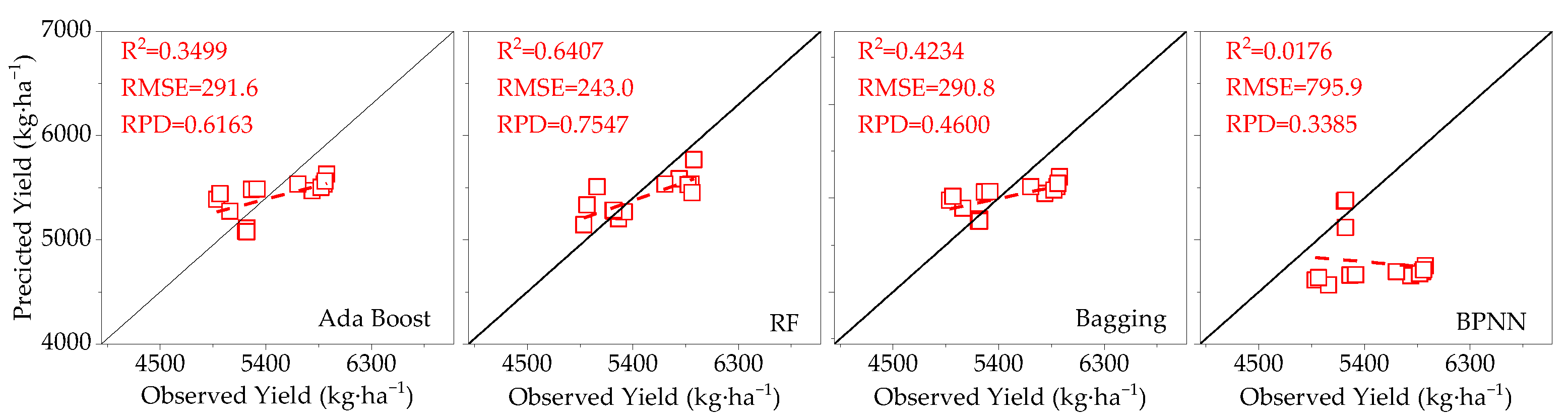
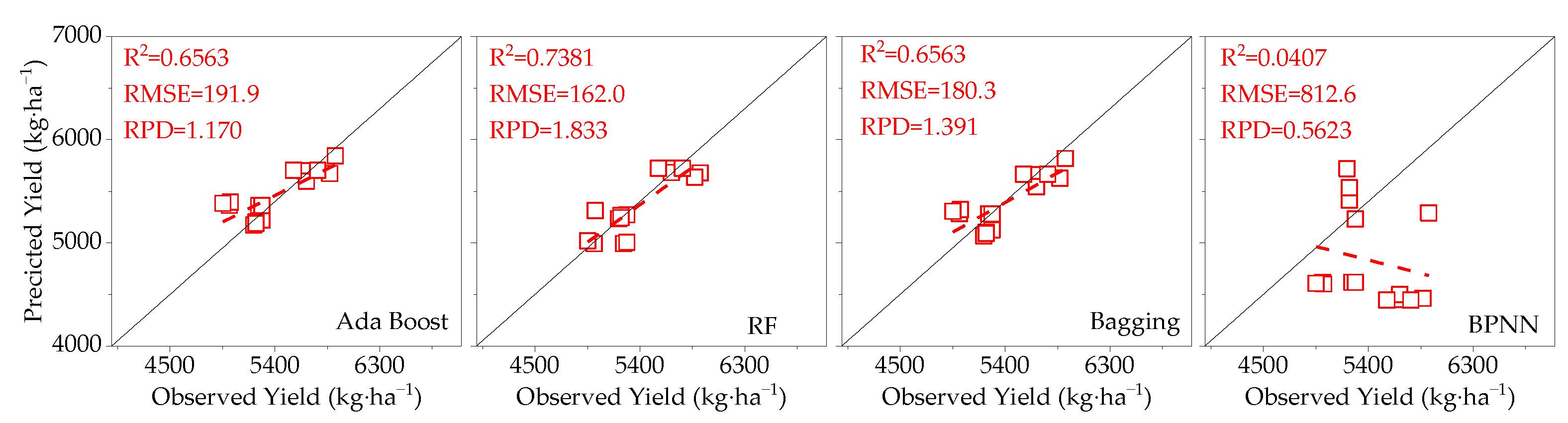
3.3.2. Construction of Cotton Yield Estimation Model Based on Canopy SIFy

The variation in canopy SIFy with respect to the cotton yield estimation model R² is shown in Figure 10. In the four key growth periods, the effect of the cotton yield model constructed with RF was the best, and the R² was basically 0.90 in each period. The R² of the cotton yield model constructed using Ada Boost and Bagging had a significant peak at 14:00–15:00, and the range of R² was 0.75–0.85. The model of cotton yield based on BPNN had the worst effect, with an R² of less than 0.5. The model R² was at its maximum during all four reproductive periods at 14:00–15:00. This indicates that the canopy-based cotton yield model utilizing SIFy at 14:00–15:00 worked best.

Yield estimation models for constructing cotton canopy SIFy were based on 14:00–15:00 in the different growth periods (Figure 11, Figure 12, Figure 13 and Figure 14). Comparison of the four modeling methods demonstrated that the cotton yield model constructed using RF was the most effective (Figure 12). The best modeling effect was achieved by using the RF algorithm in the flowering and boll period (R² = 0.9612, RMSE = 66.27 kg·ha⁻¹, RPD = 4.264, Figure 12c), followed by the flowering period (R² = 0.9590, Figure 12b). The modeling effect of the BPNN algorithm in each growth period was not very good (Figure 14), with the maximum R² value being 0.4377 (Figure 14a). The Ada Boost algorithm was used to achieve the best modeling effect in the flowering and boll period (R² = 0.8796, RMSE = 110.1 kg·ha⁻¹, RPD = 2.452, Figure 11c), along with the Bagging algorithm which also achieved the best modeling effect in the flowering and boll period (R² = 0.8898, RMSE = 102.7 kg·ha⁻¹, RPD = 2.760, Figure 13c). In the cotton yield model constructed by the four algorithms, the modeling effect was the best in the flowering and boll period, followed by the flowering period, and was the worst in the boll period. A comparison of the modeling results of the different algorithms for the different growth periods revealed that the optimal model was the one that was applied during the cotton flowering and boll period using the RF algorithm.

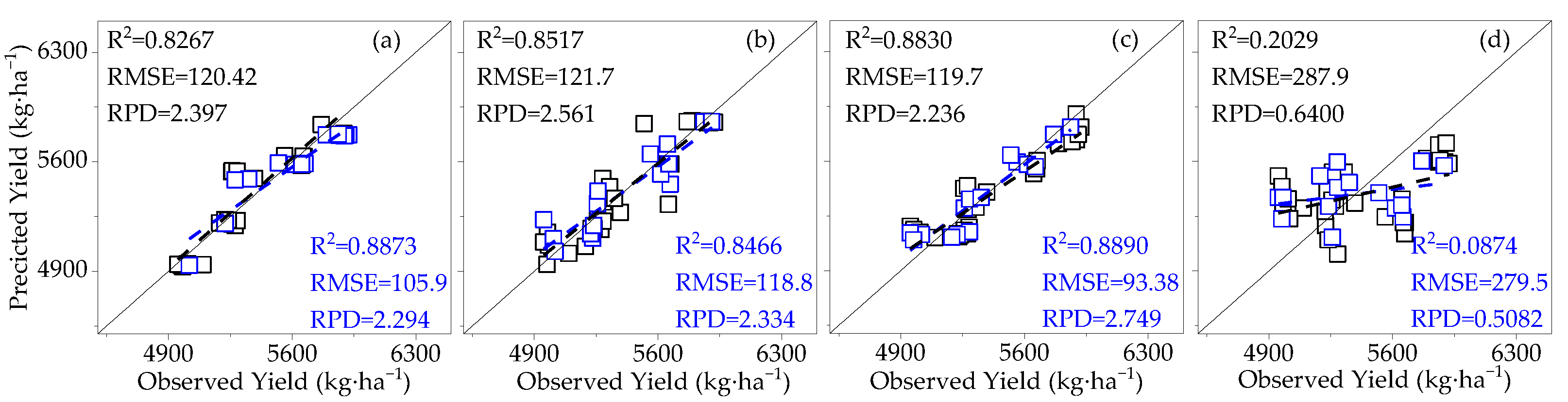
3.4. Model Validation

To verify the applicability of the model, the cotton yield estimation model based on SIF was validated in the flowering and boll period. The model was validated using data from 2023. Among them, the RF model had the best verification effect (R² = 0.6407, RMSE = 243.0 kg·ha⁻¹, RPD = 0.7547, Figure 15), followed by the Bagging model (R² = 0.4234, RMSE = 290.8 kg·ha⁻¹, RPD = 0.4600, Figure 15). The model validation effect was the worst in the BPNN model. The cotton yield estimation model based on SIFy was validated. The RF model had the best verification effect (R² = 0.7381, RMSE = 162.0 kg·ha⁻¹, RPD = 1.833, Figure 16), followed by the Bagging model (R² = 0.6563, RMSE = 180.3 kg·ha⁻¹, RPD = 1.391, Figure 16).

4. Discussion

The results of this study showed that AGB and LAI, which were significantly correlated with cotton yield, were also significantly correlated with canopy SIF. At present, AGB and LAI have been proven to be important biometric indices affecting cotton yield [57,58]. Cui et al. [59] found that the fluorescence relationship between the leaves and canopy at 740 nm was mainly affected by LAI. Yuma Sakai et al. [60] showed that SIF increases with LAI; then, it is saturated at LAI > 2–4 depending on the spectral wavelength. Wang et al. [42] concluded that SIF had a good relationship with aboveground biomass (R²= 0.65–0.82). These results indicate that SIF is indirectly related to the cotton yield through LAI and AGB. However, some studies have concluded that canopy SIF can be used as a crop monitoring indicator to directly estimate crop yield [23,61]. The mechanisms and indicators of SIF change in response to yield before the cotton fluffing periods are currently unclear. LAI and AGB, which represent vegetation canopy structure and organic matter accumulation, respectively, are dynamic at various periods of cotton growth. Therefore, it is important to study the relationship between cotton canopy SIF and dynamic change indicators for cotton yield estimation.

The optimal observation time for the model to estimate cotton yield based on canopy SIF was 14:00–15:00. The diurnal variation in cotton canopy SIF was basically consistent with that of photosynthetically active radiation (PAR), which reached the maximum value from 14:00 to 15:00. The R² of canopy SIF and yield model during the day basically showed a gradual increase from 10:00 to 14:00 and a gradual decrease from 15:00 to 19:00. This may be due to the fact that 14:00–15:00 is the midday period in Xinjiang when the light intensity is the highest. PAR drives photosynthesis and excites chlorophyll fluorescence [62]. SIF mainly responds to changes in PAR rather than actual changes in photosynthetic efficiency, and thus, photosynthetically active radiation is a key driver of SIF [63,64]. It has been shown that PAR is one of the main sources of SIF inversion errors [65,66]. Therefore, in this study, PAR was used to normalize SIF to mitigate the effect of light intensity on SIF. The optimal time for the R² for the canopy-based SIFy estimation yield model for cotton with PAR effects removed was also 14:00–15:00.

The optimum growth period for yield estimation using both SIF and SIFy was during the flowering and boll period with R² values of 0.9422 and 0.9671. The effects of LAI and AGB on cotton canopy SIF and cotton yield were similar. During the whole growth period, LAI and AGB increased from the budding period to the flowering and boll period but decreased in the boll period. The correlation of LAI and AGB with cotton yield and SIF was elevated from the budding period, reached a maximum during the flowering and boll period, and declined during the boll period. The trend of the R² of the cotton yield model based on SIF and SIFy basically follows the pattern of LAI and AGB. It shows that LAI and AGB are factors that influence the SIF and yield models. This may be because when LAI and AGB increase, cotton is in a vigorous growth period, and due to the scattering and reabsorption effects inside the leaves and canopy [67], the SIF obtained from the canopy will also increase with the increase in light area. When LAI and AGB decreased, some cotton leaves fell off, resulting in a decrease in light area and AGB. In the boll period, cotton approaches maturity, leaves gradually age, and non-photochemical quenching (NPQ) increases [68], leading to a decrease in the correlation between SIF and yield, which increases the uncertainty of the SIF yield model in the later growth period. The photosynthetic area of cotton reaches its maximum in the flowering and boll period, and the accumulation of photosynthetic substances at this stage may be a key factor in determining cotton yield [69].

Compared with SIF, SIFy can better estimate the cotton yield. In the estimation of cotton yield by SIFy, the RF model had the best effect (R² = 0.9612, RMSE = 66.27 kg·ha⁻¹, RPD = 4.264), followed by Ada Boost, whereas BPNN had the worst effect. The model was verified with the data of 2023, and the applicability of the model was proved. Cai et al. [70] estimated the yield of a major crop (wheat) in Australia using satellite SIF data based on machine learning (ML) methods such as RF and SVM, and the Random Forest algorithm achieved high-performance yield prediction (R² = 0.75). Many studies have shown that RF outperforms other machine learning methods for crop yield estimation [71]. Cao et al. [72] estimated rice yield using three methods: linear, ML, and deep learning. Among these, the best results were obtained using a Random Forest model with R² = 0.76–0.82 and RMSE = 366.0–723.3 kg·ha⁻¹. PAR data can eliminate the effect of SIF due to light instability. This method can extract a more accurate and reliable SIF data set from long-term field observations for studying the relationship between SIF and vegetation photosynthesis [73]. SIF can better estimate yield after PAR normalization [74,75].

The relationship between SIF and yield is complicated. In this study, SIF was used to directly estimate cotton yield, and although AGB and LAI, which are significantly correlated with cotton yield and canopy SIF, were utilized for interpretation, other indicators, such as chlorophyll content, canopy leaf structure, and other biometric parameters, also influenced SIF production. Therefore, it is necessary to analyze the interaction process between incident light and vegetation in detail, to identify the reasons affecting SIF and photosynthesis, and better explain the relationship between SIF and yield from the mechanism. In this study, the PAR-normalized SIF was used to eliminate the effect of PAR on SIF, resulting in improved accuracy of yield estimation models for cotton. In this study, the normalization of SIF was used to eliminate the effect of PAR on SIF so that the accuracy of the yield estimation model for cotton was improved. However, environmental factors such as solar zenith angle, moisture, air temperature, and vapor pressure difference (VPD) affect the process of SIF generation, and further study is required to eliminate the effects of environmental factors on SIF and thus improve the quality of SIF data. In this study, cotton yield was estimated based on the hourly scale of cotton in the ground canopy. Different time and spatial scales create uncertainty in the relationship between SIF and cotton yield, where the optimal observation requires further investigation.

5. Conclusions

In this study, we analyzed the biometric parameters affecting the correlation between cotton canopy SIF and yield, clarified the optimal time and growth period for yield estimation by cotton canopy SIF, and established and screened the optimal model for yield estimation by using cotton canopy SIF parameters. Our conclusions based on this research are as follows:

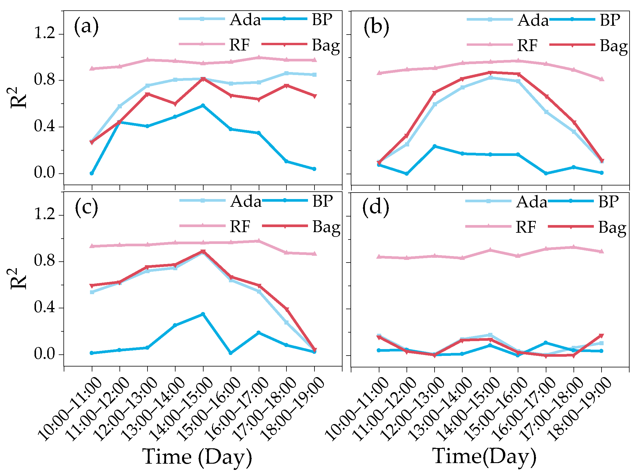
• The effects of LAI and AGB on cotton canopy SIF and cotton yield were similar. Throughout the reproductive period of cotton, the LAI, AGB, and canopy SIF all gradually increased from the budding period to the flowering and boll period and began to decline in the boll period. The correlation coefficients of LAI and AGB with cotton yield and canopy SIF both increased from the budding period, reached a maximum during the flowering and boll period, and decreased in the boll period, all of which were significantly positively correlated. The trend of the R² of the cotton yield model based on SIF and SIFy closely follows the pattern of LAI and AGB;
• At different monitoring time periods, the R² of the cotton yield estimation model based on SIF and SIFy showed a gradual increase from 10:00 to 14:00 and a gradual decrease from 15:00 to 19:00, and the optimal observation time for the cotton canopy SIF to estimate the yield was 14:00–15:00. The R² of the cotton yield model based on SIF and SIFy increased with the course of fertility from the budding period to the flowering and boll period and decreased in the boll period, and the optimal growth period for the estimation model was the flowering and boll period;
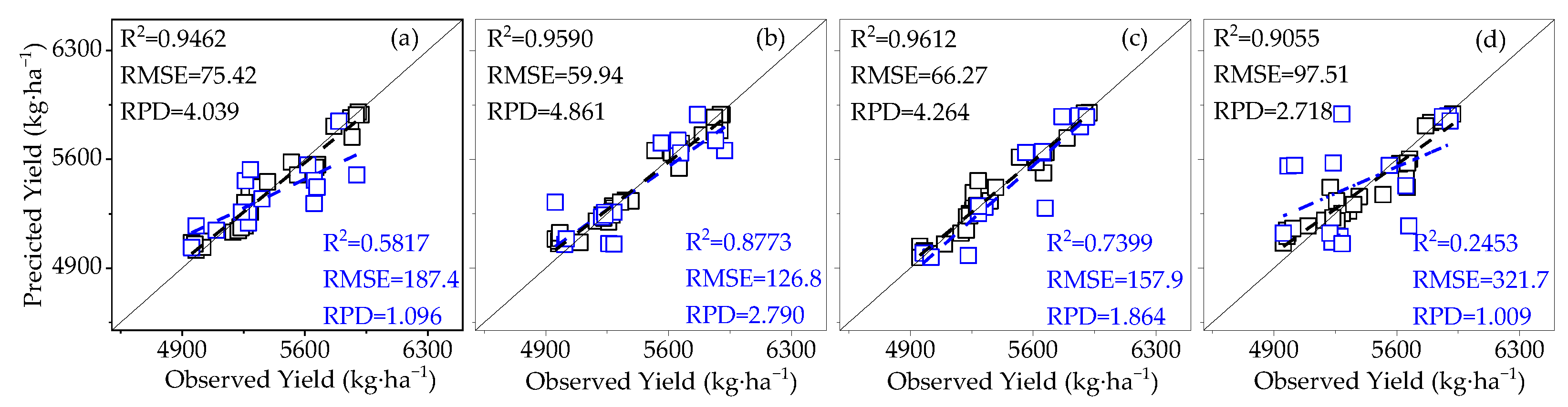
• Compared to SIF, SIFy has a superior estimation of yield. The best yield estimation model based on the RF algorithm for canopy SIFy parameters at 14:00–15:00 during the flowering and boll period (R² = 0.9612, RMSE = 66.27 kg·ha⁻¹, RPD = 4.264) was followed by the model utilizing the Bagging algorithm (R² = 0.8898) and the Ada Boost algorithm (R² = 0.8796). Through verification, the applicability of the model is proved.

References

- Abdelraheem, A.; Esmaeili, N.; O’Connell, M.; Zhang, J.F. Progress and perspective on drought and salt stress tolerance in cotton. Ind. Crops Prod. 2019, 130, 118–129. [Google Scholar] [CrossRef]
- Ashapure, A.; Jung, J.H.; Chang, A.J.; Oh, S.; Yeom, J.; Maeda, M.; Maeda, A.; Dube, N.; Landivar, J.; Hague, S.; et al. Developing a machine learning based cotton yield estimation framework using multi-temporal UAS data. ISPRS-J. Photogramm. Remote Sens. 2020, 169, 180–194. [Google Scholar] [CrossRef]
- Pazhanivelan, S.; Kumaraperumal, R.; Shanmugapriya, P.; Sudarmanian, N.S.; Sivamurugan, A.P.; Satheesh, S. Quantification of Biophysical Parameters and Economic Yield in Cotton and Rice Using Drone Technology. Agriculture 2023, 13, 1668. [Google Scholar] [CrossRef]
- Singh, J.; Gamble, A.V.; Brown, S.; Campbell, B.T.; Jenkins, J.; Koebernick, J.; Bartley, P.C.; Sanz-Saez, A. 65 years of cotton lint yield progress in the USA: Uncovering key influential yield components. Field Crops Res. 2023, 302, 10. [Google Scholar] [CrossRef]
- Ibrahim, I.A.E.; Yehia, W.M.B.; Saleh, F.H.; Lamlom, S.F.; Ghareeb, R.Y.; El-Banna, A.A.A.; Abdelsalam, N.R. Impact of Plant Spacing and Nitrogen Rates on Growth Characteristics and Yield Attributes of Egyptian Cotton (Gossypium barbadense L.). Front. Plant Sci. 2022, 13, 916734. [Google Scholar] [CrossRef] [PubMed]
- Rodriguez-Sanchez, J.; Li, C.; Paterson, A.H. Cotton Yield Estimation From Aerial Imagery Using Machine Learning Approaches. Front. Plant Sci. 2022, 13, 870181. [Google Scholar] [CrossRef] [PubMed]
- Mikhailenko, I.M. Estimation of Parameters of Biomass State of Sowing Spring Wheat. Remote Sens. 2022, 14, 1388. [Google Scholar] [CrossRef]
- Sishodia, R.P.; Ray, R.L.; Singh, S.K. Applications of Remote Sensing in Precision Agriculture: A Review. Remote Sens. 2020, 12, 3136. [Google Scholar] [CrossRef]
- Karthikeyan, L.; Chawla, I.; Mishra, A.K. A review of remote sensing applications in agriculture for food security: Crop growth and yield, irrigation, and crop losses. J. Hydrol. 2020, 586, 22. [Google Scholar] [CrossRef]
- Suarez, L.A.; Robson, A.; McPhee, J.; O’Halloran, J.; van Sprang, C. Accuracy of carrot yield forecasting using proximal hyperspectral and satellite multispectral data. Precis. Agric. 2020, 21, 1304–1326. [Google Scholar] [CrossRef]
- Noda, H.M.; Muraoka, H.; Nasahara, K.N. Plant ecophysiological processes in spectral profiles: Perspective from a deciduous broadleaf forest. J. Plant Res. 2021, 134, 737–751. [Google Scholar] [CrossRef]
- Terentev, A.; Dolzhenko, V.; Fedotov, A.; Eremenko, D. Current State of Hyperspectral Remote Sensing for Early Plant Disease Detection: A Review. Sensors 2022, 22, 757. [Google Scholar] [CrossRef]
- Pokhrel, A.; Virk, S.; Snider, J.L.; Vellidis, G.; Hand, L.C.; Sintim, H.Y.; Parkash, V.; Chalise, D.P.; Lee, J.M.; Byers, C. Estimating yield-contributing physiological parameters of cotton using UAV-based imagery. Front. Plant Sci. 2023, 14, 22. [Google Scholar] [CrossRef]
- Pandya, P.; Gontia, N.K. Early crop yield prediction for agricultural drought monitoring using drought indices, remote sensing, and machine learning techniques. J. Water Clim. Change 2023, 18, 4729–4746. [Google Scholar] [CrossRef]
- Han, P.; Zhai, Y.P.; Liu, W.H.; Lin, H.R.; An, Q.S.; Zhang, Q.; Ding, S.G.; Zhang, D.W.; Pan, Z.Y.; Nie, X.H. Dissection of Hyperspectral Reflectance to Estimate Photosynthetic Characteristics in Upland Cotton (Gossypium hirsutum L.) under Different Nitrogen Fertilizer Application Based on Machine Learning Algorithms. Plants 2023, 12, 455. [Google Scholar] [CrossRef] [PubMed]
- Banerjee, B.P.; Spangenberg, G.; Kant, S. CBM: An IoT Enabled LiDAR Sensor for In-Field Crop Height and Biomass Measurements. Biosensors 2022, 12, 16. [Google Scholar] [CrossRef] [PubMed]
- Luo, L.; Sun, S.K.; Xue, J.; Gao, Z.H.; Zhao, J.F.; Yin, Y.L.; Gao, F.; Luan, X.B. Crop yield estimation based on assimilation of crop models and remote sensing data: A systematic evaluation. Agric. Syst. 2023, 210, 17. [Google Scholar] [CrossRef]
- Muruganantham, P.; Wibowo, S.; Grandhi, S.; Samrat, N.H.; Islam, N. A Systematic Literature Review on Crop Yield Prediction with Deep Learning and Remote Sensing. Remote Sens. 2022, 14, 1990. [Google Scholar] [CrossRef]
- Skakun, S.; Kalecinski, N.I.; Brown, M.G.L.; Johnson, D.M.; Vermote, E.F.; Roger, J.-C.; Franch, B. Assessing within-Field Corn and Soybean Yield Variability from WorldView-3, Planet, Sentinel-2, and Landsat 8 Satellite Imagery. Remote Sens. 2021, 13, 872. [Google Scholar] [CrossRef]
- Jia, M.; Colombo, R.; Rossini, M.; Celesti, M.; Zhu, J.; Cogliati, S.; Cheng, T.; Tian, Y.; Zhu, Y.; Cao, W.; et al. Estimation of leaf nitrogen content and photosynthetic nitrogen use efficiency in wheat using sun-induced chlorophyll fluorescence at the leaf and canopy scales. Eur. J. Agron. 2021, 122, 126192. [Google Scholar] [CrossRef]
- Muhammad, I.; Shalmani, A.; Ali, M.; Yang, Q.H.; Ahmad, H.; Li, F.B. Mechanisms Regulating the Dynamics of Photosynthesis Under Abiotic Stresses. Front. Plant Sci. 2021, 11, 25. [Google Scholar] [CrossRef]
- Mu, X.H.; Chen, Y.L. The physiological response of photosynthesis to nitrogen deficiency. Plant Physiol. Biochem. 2021, 158, 76–82. [Google Scholar] [CrossRef]
- Somkuti, P.; Bösch, H.; Feng, L.; Palmer, P.I.; Parker, R.J.; Quaife, T. A new space-borne perspective of crop productivity variations over the US Corn Belt. Agric. For. Meteorol. 2020, 281, 11. [Google Scholar] [CrossRef]
- Mohammed, G.H.; Colombo, R.; Middleton, E.M.; Rascher, U.; van der Tol, C.; Nedbal, L.; Goulas, Y.; Perez-Priego, O.; Damm, A.; Meroni, M.; et al. Remote sensing of solar-induced chlorophyll fluorescence (SIF) in vegetation: 50 years of progress. Remote Sens. Environ. 2019, 231, 111177. [Google Scholar] [CrossRef]
- Kimm, H.; Guan, K.Y.; Burroughs, C.H.; Peng, B.; Ainsworth, E.A.; Bernacchi, C.J.; Moore, C.E.; Kumagai, E.; Yang, X.; Berry, J.A.; et al. Quantifying high-temperature stress on soybean canopy photosynthesis: The unique role of sun-induced chlorophyll fluorescence. Glob. Change Biol. 2021, 27, 2403–2415. [Google Scholar] [CrossRef]
- Marrs, J.K.; Reblin, J.S.; Logan, B.A.; Allen, D.W.; Reinmann, A.B.; Bombard, D.M.; Tabachnik, D.; Hutyra, L.R. Solar-Induced Fluorescence Does Not Track Photosynthetic Carbon Assimilation Following Induced Stomatal Closure. Geophys. Res. Lett. 2020, 47, e2020GL087956. [Google Scholar] [CrossRef]
- Bacour, C.; Maignan, F.; MacBean, N.; Porcar-Castell, A.; Flexas, J.; Frankenberg, C.; Peylin, P.; Chevallier, F.; Vuichard, N.; Bastrikov, V. Improving Estimates of Gross Primary Productivity by Assimilating Solar-Induced Fluorescence Satellite Retrievals in a Terrestrial Biosphere Model Using a Process-Based SIF Model. J. Geophys. Res. Biogeosci. 2019, 26, 3281–3306. [Google Scholar] [CrossRef]
- Campbell, P.K.E.; Huemmrich, K.F.; Middleton, E.M.; Ward, L.A.; Julitta, T.; Daughtry, C.S.T.; Burkart, A.; Russ, A.L.; Kustas, W.P. Diurnal and Seasonal Variations in Chlorophyll Fluorescence Associated with Photosynthesis at Leaf and Canopy Scales. Remote Sens. 2019, 11, 488. [Google Scholar] [CrossRef]
- Zeng, Y.L.; Badgley, G.; Dechant, B.; Ryu, Y.; Chen, M.; Berry, J.A. A practical approach for estimating the escape ratio of near-infrared solar-induced chlorophyll fluorescence. Remote Sens. Environ. 2019, 232, 14. [Google Scholar] [CrossRef]
- Liu, J.G.; Huffman, T.; Qian, B.D.; Shang, J.L.; Li, Q.M.; Dong, T.F.; Davidson, A.; Jing, Q. Crop Yield Estimation in the Canadian Prairies Using Terra/MODIS-Derived Crop Metrics. IEEE J. Sel. Top. Appl. Earth Observ. Remote Sens. 2020, 13, 2685–2697. [Google Scholar] [CrossRef]
- Marshall, M.; Tu, K.; Brown, J. Optimizing a remote sensing production efficiency model for macro-scale GPP and yield estimation in agroecosystems. Remote Sens. Environ. 2018, 217, 258–271. [Google Scholar] [CrossRef]
- He, L.Y.; Magney, T.; Dutta, D.; Yin, Y.; Köhler, P.; Grossmann, K.; Stutz, J.; Dold, C.; Hatfield, J.; Guan, K.Y.; et al. From the Ground to Space: Using Solar-Induced Chlorophyll Fluorescence to Estimate Crop Productivity. Geophys. Res. Lett. 2020, 47, 12. [Google Scholar] [CrossRef]
- Sloat, L.L.; Lin, M.; Butler, E.E.; Johnson, D.; Holbrook, N.M.; Huybers, P.J.; Lee, J.E.; Mueller, N.D. Evaluating the benefits of chlorophyll fluorescence for in-season crop productivity forecasting. Remote Sens. Environ. 2021, 260, 14. [Google Scholar] [CrossRef]
- Guan, K.; Berry, J.A.; Zhang, Y.; Joiner, J.; Guanter, L.; Badgley, G.; Lobell, D.B. Improving the monitoring of crop productivity using spaceborne solar-induced fluorescence. Glob. Change Biol. 2016, 22, 716–726. [Google Scholar] [CrossRef]
- Joshi, A.; Pradhan, B.; Chakraborty, S.; Behera, M.D. Winter wheat yield prediction in the conterminous United States using solar-induced chlorophyll fluorescence data and XGBoost and random forest algorithm. Ecol. Inform. 2023, 77, 102194. [Google Scholar] [CrossRef]
- Nichol, C.J.; Drolet, G.; Porcar-Castell, A.; Wade, T.; Sabater, N.; Middleton, E.M.; MacLellan, C.; Levula, J.; Mammarella, I.; Vesala, T.; et al. Diurnal and Seasonal Solar Induced Chlorophyll Fluorescence and Photosynthesis in a Boreal Scots Pine Canopy. Remote Sens. 2019, 11, 273. [Google Scholar] [CrossRef]
- Yang, P.Q.; van der Tol, C.; Campbell, P.K.E.; Middleton, E.M. Fluorescence Correction Vegetation Index (FCVI): A physically based reflectance index to separate physiological and non-physiological information in far-red sun-induced chlorophyll fluorescence. Remote Sens. Environ. 2020, 240, 16. [Google Scholar] [CrossRef]
- Yoshida, Y.; Joiner, J.; Tucker, C.; Berry, J.; Lee, J.E.; Walker, G.; Reichle, R.; Koster, R.; Lyapustin, A.; Wang, Y. The 2010 Russian drought impact on satellite measurements of solar-induced chlorophyll fluorescence: Insights from modeling and comparisons with parameters derived from satellite reflectances. Remote Sens. Environ. 2015, 166, 163–177. [Google Scholar] [CrossRef]
- Dechant, B.; Ryu, Y.; Badgley, G.; Zeng, Y.L.; Berry, J.A.; Zhang, Y.G.; Goulas, Y.; Li, Z.H.; Zhang, Q.; Kang, M.; et al. Canopy structure explains the relationship between photosynthesis and sun-induced chlorophyll fluorescence in crops. Remote Sens. Environ. 2020, 241, 17. [Google Scholar] [CrossRef]
- Hwang, Y.; Kim, J.; Ryu, Y. Canopy structural changes explain reductions in canopy-level solar induced chlorophyll fluorescence in Prunus yedoensis seedlings under a drought stress condition. Remote Sens. Environ. 2023, 296, 15. [Google Scholar] [CrossRef]
- Wu, G.; Jiang, C.; Kimm, H.; Wang, S.; Bernacchi, C.; Moore, C.E.; Suyker, A.; Yang, X.; Magney, T.; Frankenberg, C.; et al. Difference in seasonal peak timing of soybean far-red SIF and GPP explained by canopy structure and chlorophyll content. Remote Sens. Environ. 2022, 279, 113104. [Google Scholar] [CrossRef]
- Wang, X.; Pan, S.; Pan, N.; Pan, P. Grassland productivity response to droughts in northern China monitored by satellite-based solar-induced chlorophyll fluorescence. Sci. Total Environ. 2022, 830, 154550. [Google Scholar] [CrossRef]
- Magney, T.S.; Barnes, M.L.; Yang, X. On the Covariation of Chlorophyll Fluorescence and Photosynthesis Across Scales. Geophys. Res. Lett. 2020, 47, 7. [Google Scholar] [CrossRef]
- Zhang, Y.; Guanter, L.; Berry, J.A.; van der Tol, C.; Yang, X.; Tang, J.; Zhang, F. Model-based analysis of the relationship between sun-induced chlorophyll fluorescence and gross primary production for remote sensing applications. Remote Sens. Environ. 2016, 187, 145–155. [Google Scholar] [CrossRef]
- Peng, B.; Guan, K.; Zhou, W.; Jiang, C.; Frankenberg, C.; Sun, Y.; He, L.; Kohler, P. Assessing the benefit of satellite-based Solar-Induced Chlorophyll Fluorescence in crop yield prediction. Int. J. Appl. Earth Obs. Geoinf. 2020, 90, 102126. [Google Scholar] [CrossRef]
- Condran, S.; Bewong, M.; Islam, M.Z.; Maphosa, L.; Zheng, L. Machine Learning in Precision Agriculture: A Survey on Trends, Applications and Evaluations Over Two Decades. IEEE Access 2022, 10, 73786–73803. [Google Scholar] [CrossRef]
- Liu, Y.; Wang, S.; Wang, X.; Chen, B.; Chen, J.; Wang, J.; Huang, M.; Wang, Z.; Ma, L.; Wang, P.; et al. Exploring the superiority of solar-induced chlorophyll fluorescence data in predicting wheat yield using machine learning and deep learning methods. Comput. Electron. Agric. 2022, 192, 106612. [Google Scholar] [CrossRef]
- Wang, Y.-Q.; Leng, P.; Shang, G.-F.; Zhang, X.; Li, Z.-L. Sun-induced chlorophyll fluorescence is superior to satellite vegetation indices for predicting summer maize yield under drought conditions. Comput. Electron. Agric. 2023, 205, 107615. [Google Scholar] [CrossRef]
- Meroni, M.; Waldner, F.; Seguini, L.; Kerdiles, H.; Rembold, F. Yield forecasting with machine learning and small data: What gains for grains? Agric. For. Meteorol. 2021, 308, 13. [Google Scholar] [CrossRef]
- Liu, Z.G.; He, X.; Yang, P.Q.; Jiang, H.; Xu, S.; Zhao, H.R.; Ren, S.X.; Chen, M. Diurnal Pattern of Sun-Induced Chlorophyll Fluorescence as Reliable Indicators of Crop Water Stress. IEEE Geosci. Remote Sens. Lett. 2023, 20, 5. [Google Scholar] [CrossRef]
- Damm, A.; Erler, A.; Hillen, W.; Meroni, M.; Schaepman, M.E.; Verhoef, W.; Rascher, U. Modeling the impact of spectral sensor configurations on the FLD retrieval accuracy of sun-induced chlorophyll fluorescence. Remote Sens. Environ. 2011, 115, 1882–1892. [Google Scholar] [CrossRef]
- Daumard, F.; Goulas, Y.; Champagne, S.; Fournier, A.; Ounis, A.; Olioso, A.; Moya, I. Continuous Monitoring of Canopy Level Sun-Induced Chlorophyll Fluorescence During the Growth of a Sorghum Field. IEEE Trans. Geosci. Remote Sens. 2012, 50, 4292–4300. [Google Scholar] [CrossRef]
- Freund, Y.; Schapire, R.E. A decision-theoretic generalization of on-line learning and an application to boosting. J. Comput. Syst. Sci. 1997, 55, 119–139. [Google Scholar] [CrossRef]
- Pino-Mejias, R.; Jimenez-Gamero, M.-D.; Cubiles-de-la-Vega, M.-D.; Pascual-Acosta, A. Reduced bootstrap aggregating of learning algorithms. Pattern Recognit. Lett. 2008, 29, 265–271. [Google Scholar] [CrossRef]
- Breiman, L. Random Forests. Mach. Learn. 2001, 45, 5–32. [Google Scholar] [CrossRef]
- Irmak, A.; Jones, J.W.; Batchelor, W.D.; Irmak, S.; Boote, K.J.; Paz, J.O. Artificial neural network model as a data analysis tool in precision farming. Trans. ASABE 2006, 49, 2027–2037. [Google Scholar] [CrossRef]
- Grundy, P.R.; Yeates, S.J.; Bell, K.L. Cotton production during the tropical monsoon season. II—Biomass accumulation, partitioning and RUE in response to boll loss and compensation. Field Crops Res. 2020, 255, 11. [Google Scholar] [CrossRef]
- He, L.M.; Mostovoy, G. Cotton Yield Estimate Using Sentinel-2 Data and an Ecosystem Model over the Southern US. Remote Sens. 2019, 11, 2000. [Google Scholar] [CrossRef]
- Cui, T.X.; Sun, R.; Xiao, Z.Q.; Liang, Z.Y.; Wang, J. Simulating spatially distributed solar-induced chlorophyll fluorescence using a BEPS-SCOPE coupling framework. Agric. For. Meteorol. 2020, 295, 20. [Google Scholar] [CrossRef]
- Sakai, Y.; Kobayashi, H.; Kato, T. FLiES-SIF version 1.0: Three-dimensional radiative transfer model for estimating solar induced fluorescence. Geosci. Model Dev. 2020, 13, 4041–4066. [Google Scholar] [CrossRef]
- Song, L.; Guanter, L.; Guan, K.Y.; You, L.Z.; Huete, A.; Ju, W.M.; Zhang, Y.G. Satellite sun-induced chlorophyll fluorescence detects early response of winter wheat to heat stress in the Indian Indo-Gangetic Plains. Glob. Change Biol. 2018, 24, 4023–4037. [Google Scholar] [CrossRef]
- Wang, N.; Suomalainen, J.; Bartholomeus, H.; Kooistra, L.; Masiliunas, D.; Clevers, J.G.P.W. Diurnal variation of sun-induced chlorophyll fluorescence of agricultural crops observed from a point-based spectrometer on a UAV. Int. J. Appl. Earth Obs. Geoinf. 2021, 96, 102276. [Google Scholar] [CrossRef]
- Cheng, X.; Zhou, Y.; Hu, M.; Wang, F.; Huang, H.; Zhang, J. The Links between Canopy Solar-Induced Chlorophyll Fluorescence and Gross Primary Production Responses to Meteorological Factors in the Growing Season in Deciduous Broadleaf Forest. Remote Sens. 2021, 13, 2363. [Google Scholar] [CrossRef]
- Goulas, Y.; Fournier, A.; Daumard, F.; Champagne, S.; Ounis, A.; Marloie, O.; Moya, I. Gross Primary Production of a Wheat Canopy Relates Stronger to Far Red Than to Red Solar-Induced Chlorophyll Fluorescence. Remote Sens. 2017, 9, 97. [Google Scholar] [CrossRef]
- Joiner, J.; Yoshida, Y.; Köehler, P.; Campbell, P.; Frankenberg, C.; van der Tol, C.; Yang, P.Q.; Parazoo, N.; Guanter, L.; Sun, Y. Systematic Orbital Geometry-Dependent Variations in Satellite Solar-Induced Fluorescence (SIF) Retrievals. Remote Sens. 2020, 12, 2346. [Google Scholar] [CrossRef]
- Loayza, H.; Moya, I.; Quiroz, R.; Ounis, A.; Goulas, Y. Active and passive chlorophyll fluorescence measurements at canopy level on potato crops. Evidence of similitude of diurnal cycles of apparent fluorescence yields. Photosynth. Res. 2023, 155, 271–288. [Google Scholar] [CrossRef] [PubMed]
- Cordon, G.B.; Lagorio, M.G. Optical properties of the adaxial and abaxial faces of leaves.: Chlorophyll fluorescence, absorption and scattering coefficients. Photochem. Photobiol. Sci. 2007, 6, 873–882. [Google Scholar] [CrossRef] [PubMed]
- Yang, P.Q.; van der Tol, C.; Campbell, P.K.E.; Middleton, E.M. Unraveling the physical and physiological basis for the solar- induced chlorophyll fluorescence and photosynthesis relationship using continuous leaf and canopy measurements of a corn crop. Biogeosciences 2021, 18, 441–465. [Google Scholar] [CrossRef]
- Yang, G.; Tang, H.; Tong, J.; Nie, Y.; Zhang, X. Effect of fertilization frequency on cotton yield and biomass accumulation. Field Crops Res. 2012, 125, 161–166. [Google Scholar] [CrossRef]
- Cai, Y.P.; Guan, K.Y.; Lobell, D.; Potgieter, A.B.; Wang, S.W.; Peng, J.; Xu, T.F.; Asseng, S.; Zhang, Y.G.; You, L.Z.; et al. Integrating satellite and climate data to predict wheat yield in Australia using machine learning approaches. Agric. For. Meteorol. 2019, 274, 144–159. [Google Scholar] [CrossRef]
- Gopal, P.S.M.; Bhargavi, R. Performance Evaluation of Best Feature Subsets for Crop Yield Prediction Using Machine Learning Algorithms. Appl. Artif. Intell. 2019, 33, 621–642. [Google Scholar] [CrossRef]
- Cao, J.; Zhang, Z.; Tao, F.; Zhang, L.; Luo, Y.; Zhang, J.; Han, J.; Xie, J. Integrating Multi-Source Data for Rice Yield Prediction across China using Machine Learning and Deep Learning Approaches. Agric. For. Meteorol. 2021, 297, 108275. [Google Scholar] [CrossRef]
- Han, S.; Liu, Z.; Chen, Z.; Jiang, H.; Xu, S.; Zhao, H.; Ren, S. Using High-Frequency PAR Measurements to Assess the Quality of the SIF Derived from Continuous Field Observations. Remote Sens. 2022, 14, 2083. [Google Scholar] [CrossRef]
- Liu, X.; Liu, Z.; Liu, L.; Lu, X.; Chen, J.; Du, S.; Zou, C. Modelling the influence of incident radiation on the SIF-based GPP estimation for maize. Agric. For. Meteorol. 2021, 307, 108522. [Google Scholar] [CrossRef]
- Xu, S.; Liu, Z.; Han, S.; Chen, Z.; He, X.; Zhao, H.; Ren, S. Exploring the Sensitivity of Solar-Induced Chlorophyll Fluorescence at Different Wavelengths in Response to Drought. Remote Sens. 2023, 15, 1077. [Google Scholar] [CrossRef]