1. Introduction
Aboveground vegetation biomass is a key indicator of an ecosystem’s structure and function. Early forecasting of aboveground vegetation biomass is crucial for vegetation management and food security, as it could provide stakeholders and planners with an important tool to make more informed decisions and strategically address potential issues that could arise from shortages [
1,
2,
3]. Furthermore, since aboveground vegetation biomass provides vital ecosystem services, early forecasting of vegetation biomass is essential for sustainable vegetation management [
4,
5]. Moreover, vegetation biomass management is essential for climate change mitigation since it plays an important role in the carbon cycle and the collection and storage of greenhouse gas emissions from a variety of human activities and industrial processes [
2]. While aboveground vegetation biomass alone doesn’t store all emissions, it does significantly contribute to carbon sequestration, helping to offset the impact of certain emissions. This underscores the significance of effective vegetation biomass management as a part of comprehensive climate change strategies. For these reasons, aboveground vegetation biomass prediction has been the topic of multiple studies and publications [
6,
7]. These studies have developed multiple statistical and physical-based predictive models that achieved moderate to high levels of accuracy [
2,
8,
9,
10]. Despite endeavors to determine vegetation biomass indirectly via methods such as proxies or remote sensing information as opposed to direct measurements, few studies have concentrated on forecasting vegetation biomass in the near future (defined as 1–12 months) [
11,
12]. Forecasting approaches that have been utilized successfully in other disciplines (e.g., finance, hydrology) could aid in addressing the existing gap in vegetation biomass forecasting and provide early warning to pastoralists, farmers, planners, and other stakeholders on vegetation deficits that could affect livelihoods and environmental conditions.
Artificial intelligence (AI) algorithms are being increasingly employed to estimate future scenarios based on time series data in various fields such as finance [
13,
14], hydrology [
15,
16], and economics, among others [
17]. AI algorithms can address complex nonlinear problems by integrating several nonlinear transformations. Thus, AI techniques have grown in popularity among academics in recent years as they have proven effective in time series modeling by identifying patterns that humans may not see or perceive immediately [
18,
19]. Furthermore, when new data becomes available, AI models can be updated, allowing them to adapt and improve over time [
19]. The debate about the superiority of certain AI models over others is currently ongoing [
20]. Prior studies have revealed that the performance of a model is related to the time series characteristics [
19,
21]. In this regard, previous studies agree that it is necessary to conduct additional research using time series with distinct characteristics from diverse disciplines, evaluating various models, and controlling the parameters and hyperparameters of these models in order to better understand and evaluate the merits various AI models [
19,
22]. In this regard, AI models for time series forecasting of aboveground vegetation biomass have not yet been explored.
Neural networks, integral to artificial intelligence, have evolved in time series analysis with increasing efficiency. While early studies, like White’s on stock data [
23], showed modest accuracy, subsequent works [
14,
24] demonstrated significant improvements. Despite not being agriculture-focused, these studies highlighted the increasing effectiveness of neural networks across diverse domains. As vast amounts of data become available, breakthroughs in deep learning techniques and increased processing capacity of computers have enabled the development of more sophisticated neural network architectures, resulting in improved accuracy and generalization of new data. The multilayer perceptron (MLP) model, for example, which includes several hidden layers in its architecture, has been used successfully in finance, economics, hydrology, and energy-demand forecasting [
25]. The long-term memory model (LSTM) that is characterized by capturing long-term dependencies in time series has also performed well against other models in various studies, such as those by [
13] in economics and finance, [
16] in hydrology and others [
26]. The Convolutional Neural Network (CNN) model, which was initially applied to image and video recognition, segmentation, and classification, has also proven to be useful in time series analysis by capturing more relevant features without requiring manual feature engineering [
27]. CNN models outperform other DL models in studies undertaken, for example, by [
27] in finance, ref. [
28] in crop price prediction, and [
29] in health care. More developed neural network approaches have involved hybrid models that combined two or more different types of neural networks—and in some cases also statistical models—to take advantage of the strengths of each model to produce a more powerful and flexible hybrid [
30,
31]. While beyond the primary scope of this agriculture-focused research, the hybrid CNN-LSTM model exhibits superior performance across diverse disciplines, including finance, environmental engineering, atmospheric sciences [
32], and soil sciences [
30]. Similarly, across various domains—economics [
33], production planning, finance, and climatology [
34,
35]—LSTM-ARIMA consistently demonstrates superior predictive performance.
The above-mentioned studies show that debates on best time series modeling continue in diverse fields and are likely to continue for years to come. However, notwithstanding the abundance of time series modeling research, there are limited studies where these techniques have been applied to ecology, agriculture, and environmental sciences [
36], and to our knowledge, no studies using vegetation biomass time series. This study evaluates established deep learning models (MLP, GRU, LSTM, CNN, CNN-LSTM), emphasizing the hybrid CNN-LSTM for forecasting aboveground vegetation biomass with limited size data and comparing them to the classic SARIMA model. Our analysis, based on diverse neural network architectures, provides insights into handling dataset complexities. Widely used as benchmarks [
14,
31], these models enable meaningful comparisons. Focused on a specific problem domain with proven effectiveness [
22,
37,
38], the selected DL models, including MLP for simplicity, LSTM and GRU for sequential modeling, and CNN for spatial dependencies, offer a comprehensive evaluation. The hybrid CNN-LSTM model integrates spatial and temporal characteristics for a robust assessment [
31].
2. Methodology
2.1. Aboveground Biomass Database
Aboveground biomass assessment employs techniques like clip harvesting and non-destructive methods such as remote sensing and allometric equations. Monitoring stations, strategically placed based on research goals and utilizing grid patterns or clustering, operate at various scales, ranging from small plots to global observations through satellites [
1,
2,
6]. For this study, the Food and Agriculture Organization (FAO) and Texas A&M AgriLife Research (TAMU), in collaboration with the Kenya National Drought Monitoring Authority (KNDMA), have implemented a significant number of monitoring sites for aboveground biomass in grasslands and rangelands of Kenya. These monitoring sites are part of a network of sites that comprise the Predictive Livestock Early Warning System in East Africa [
4,
39]. Data from these sites were used to calibrate the Phytomass Growth Model (PHYGROW) [
39,
40] and generate near-real-time aboveground vegetation biomass time series in several strategic locations throughout Kenya [
3,
4]. The time series database employed for this study is accessible at
https://github.com/noayarae/forecasting_biomass_using_DL_models.git, accessed on 18 August 2023.
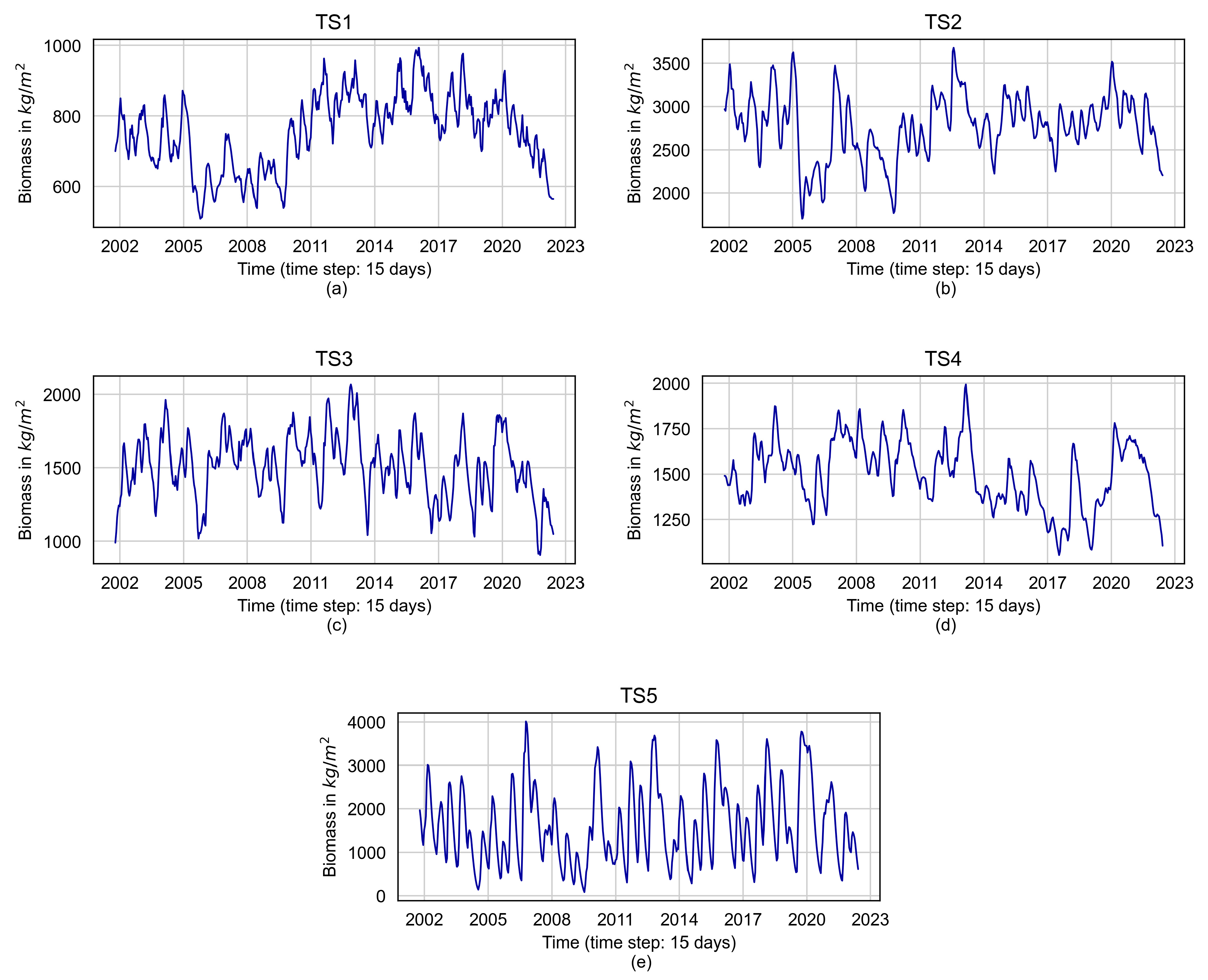
Five aboveground biomass time series were chosen for this study and will be referred to as TS1, TS2, TS3, TS4, and TS5, respectively. These included values at 15-day intervals (two values per month) from 14 January 2002 to 31 August 2022. Therefore, each time series included 496 aboveground biomass values in kg/m
2. The chosen time series were visually scrutinized to confirm the absence of any irregularities or abnormal patterns, both in terms of isolated events and chronological sequences.
Figure 1 shows the evaluated aboveground vegetation biomass time series. Significantly, these meticulously selected time series aptly capture a broad spectrum of regional aboveground biomass production, with an average low of 104.5 kg/m
2 and an average high of 3171.5 kg/m
2, effectively representing the range of production for the studied area.
2.2. Data Preprocessing
The time series
were preprocessed by normalizing them to help improve the model training process and to avoid issues such as vanishing gradients that can speed up model convergence. Normalization also helps to reduce the sensitivity of the model to the scale of the input features, improving the model’s generalization ability [
41]. Normalization was accomplished by scaling between 0 and 1 using the following equation:
where
is the time series value,
is the normalized value,
is the highest value of the time series, and
the lowest value of the time series. For subsequent applications, if new data aligns closely with the training set, the models can use the same normalization values. However, significant differences may warrant a re-evaluation and normalization using relevant values. As the initial models were trained with limited data, incorporating new data presents an opportunity for enhanced performance through retraining, ensuring continued optimal accuracy.
2.3. Modeling, Prediction, and Tool Setup
The modeling process involved a sliding window of 24 data points representing the historical aboveground biomass data over one year. The forecasting horizons included 6, 12, 18, and 24 values, equivalent to 3, 6, 9, and 12 months, respectively. These forecasting intervals were strategically chosen to align with the practical needs of stakeholders. Farmers, ranchers, and decision-makers often require long-term forecasts (one year) for planning purposes, while the 3–6-month forecasting intervals are critical for rapid decision-making to mitigate issues such as forage scarcity impacting animal health. The horizons were achieved using one-step ahead iterative prediction. Taking into account the range of forecasting horizons and the number of time series, this study encompassed a total of twenty cases, with each case involving twenty-five replications of forecasting to ensure a reliable outcome. This comprehensive approach effectively covers a spectrum of decision points, providing valuable insights applicable to various scenarios where timely actions are paramount.
2.3.1. Iterative Forecasting Approach
The iterative method is a long-established technique for performing multi-step ahead predictions. It takes the output of a one-step ahead prediction as input for the next step prediction [
18,
42]. The equation to compute the first step ahead of prediction as a function of the w preceding values is as follows:
where
is the sliding window length. The next step
would also be based on the previous
values, including the newly predicted value
:
In general, the value of p-step ahead would be.
2.3.2. Software and Computer Tools
This study utilized the NVIDIA RTX 4090 GPU, renowned for advanced architecture and parallel processing, to accelerate computational tasks. Both the DL and SARIMA models were implemented using the Python platform v3.9.13 [
43]. The DL models were built using various open-access libraries, including scipy, keras, and tensorflow, while the SARIMA model mainly relied on statsmodels. The codes developed for this study are available at
https://github.com/noayarae/forecasting_biomass_using_DL_models.git, accessed on 18 August 2023.
2.4. Learning Models—Model Implementation
2.4.1. Multilayer Perceptron (MLP)
The MLP is a type of artificial neural network composed of at least three layers: an input layer, one or more intermediate hidden layers, and an output layer [
44]. The output at each hidden layer and in the output layer is computed as follows:
where
is the activation function,
is the number of neurons,
is the matrix of weights between the
hidden layer and the
hidden layer,
is the output of the hidden neuron, and
is the vector of the output layer.
The learning process of the MLP algorithm consists of finding, using backpropagation, the weight values at each network connection (matrix of weights) to minimize the error between the output layer values and the expected values. Before the MLP learning process, the model underwent two-step manual tuning using GridSearchCV for optimal hyperparameter selection. In the initial hyperparameter optimization step, crucial learning parameters, including number of neurons, activation function, optimizer, learning rate, batch size, and epoch, were finely tuned, with details in
Table 1. Values were chosen within literature-aligned ranges, ensuring relevance and comparability. For instance, the number of neurons ranged from 50 to 400, activation functions included Relu, Sigmoid, and Tanh, and learning rates varied from 0.001 to 0.01. Batch sizes of 16, 32, and 64 were considered, with epoch numbers ranging from 100 to 500 and an early stopping of 30. In the second step, focusing on model architecture refinement, 1- and 2-layer networks were explored alongside dropout rates of 0, 0.1, 0.15, and 0.20. This comprehensive exploration, rooted in existing research, ensures an optimal model configuration balancing complexity and generalization, adhering to established practices in deep learning.
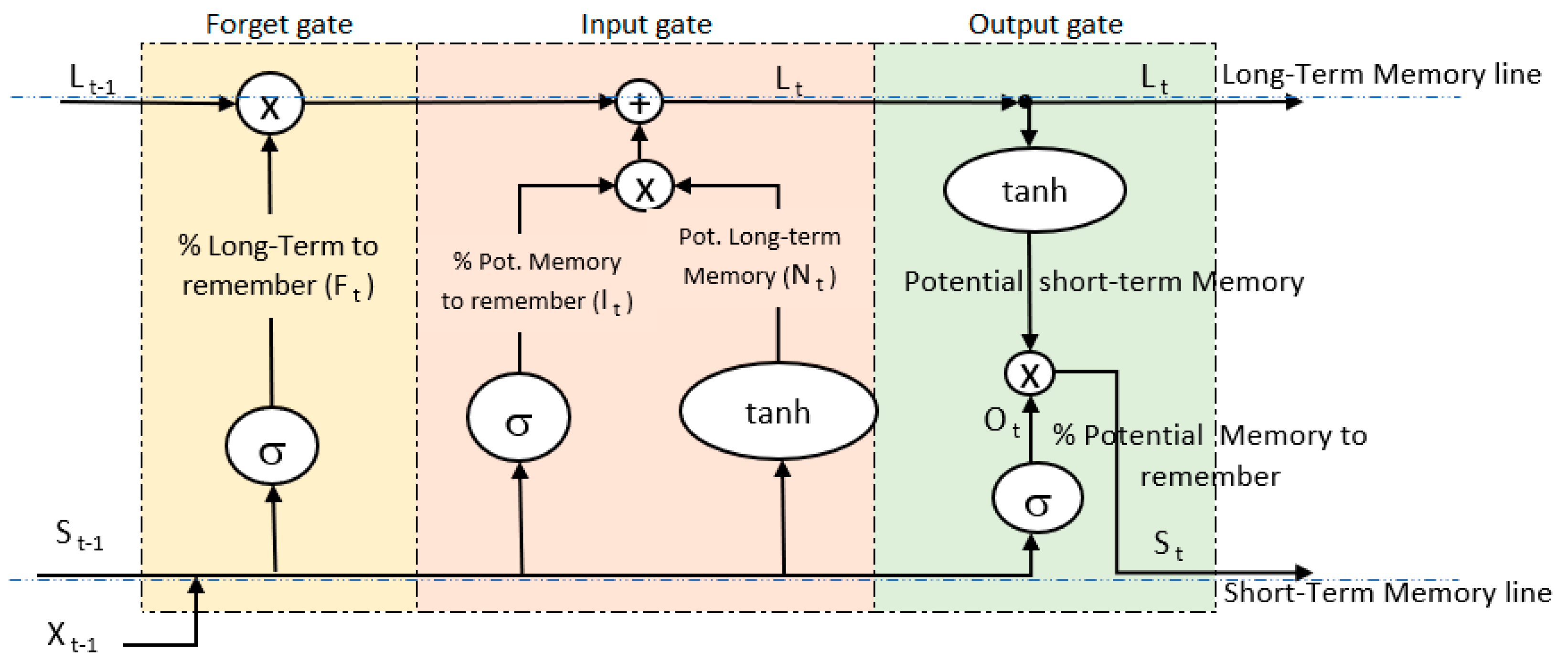
2.4.2. Long Short-Term Memory (LSTM) Network
LSTM is an enhanced type of Recurrent Neural Network (RNN) designed to model sequences and their dependencies accurately over a longer period, maintaining a single-cell structure with several modifications to the standard RNN architecture. The LSTM architecture addresses the inability of the standard RNN to remember long-term dependencies [
45]. The LSTM cell features three gates, known as Forget, Input, and Output, that control the flow of information. The Forget gate decides what information from the previous time step to discard; the Input gate determines what new information to add/learn from the current input, and the Output gate regulates what information to pass to the next time step [
18,
46].
Figure 3 shows the LSTM model architecture.
As
Figure 3 illustrates, in the first gate, the Forget gate, the LSTM decides what information to discard from the cell state using the sigmoid function. This layer considers the previous hidden state (
) and the current input (
) and, through the sigmoid function, outputs a value between 0 and 1 for each cell state in the long-term memory (
). A value of 1 means to keep the information in its entirety, while a value of 0 means to discard it completely.
In the second gate, the Input gate, the LSTM decides what new information to store in the cell state through two sub-steps: first, the input gate layer uses a sigmoid function to determine what percentage of the potential memory to add to the long-term memory. Second, the LSTM uses a function to combine the short-term memory and the input to create a potential long-term memory. The product of the two sub-step outputs is added to long-term memory to update it ().
In the third gate, the Output gate, the short-term memory is updated. Here, the new long-term memory is processed through a function to find the potential short-term memory. The LSTM then decides how much of this potential short-term memory has to pass on by multiplying a percentage computed using a sigmoid function ().
It is important to note that the LSTM memory cells utilize both addition and multiplication in transforming and transferring information. The use of addition is crucial in helping to maintain a consistent error during backpropagation. Instead of affecting the next cell state through the multiplication of the current state with new input, the two are combined through addition in the Input gate. Meanwhile, the Forget gate continues to rely on multiplication [
46].
During the training process, the initial LSTM parameter values (weights and bias) are generated arbitrarily. These parameters are updated via the standard gradient descent method using the backpropagation algorithm. The performance of this algorithm is highly dependent on the selection of optimal hyperparameters, which improves the accuracy of time-series problems [
18,
45,
46,
47]. The LSTM hyperparameters were fine-tuned manually, following a two-step process using GridSearchCV, mirroring the approach taken for MLP. The optimization encompassed the following ranges for hyperparameters: number of neurons (50 to 400), activation functions (ReLU, Tanh, and Sigmoid), optimizers (Adam and Adamax), learning rate (0.001 to 0.01), batch sizes (16, 32, 64), the number of epochs (100 to 500) with early stopping. Additionally, one-layer and two-hidden-layer networks were assessed, considering dropout rates ranging from 0 to 0.2.
Table 1 presents the optimized values.
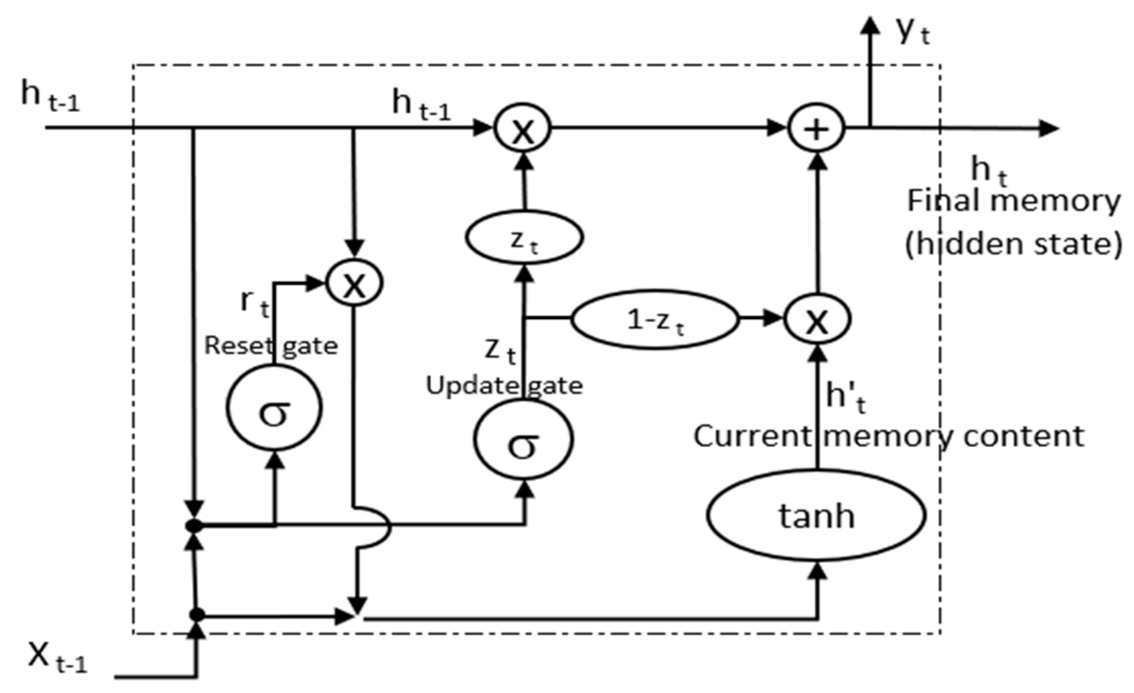
2.4.3. Gated Recurrent Unit (GRU)
The GRU algorithm is an enhanced type of RNN that addresses the issue of vanishing gradients in standard RNNs [
18]. It accomplishes this by utilizing two types of gates—an update gate and a reset gate—which are essentially two vectors that determine the relevant information to be transmitted to the output. These gates can be trained to selectively retain relevant information from previous time steps without losing value over time, as well as to eliminate irrelevant information that hinders accurate prediction [
48].
Figure 4 illustrates this process:
The Reset gate (
) determines how much of the previous hidden state should be forgotten and how much of the current input should be considered. The gate considers the previous hidden state (
) and the current input (
) and, through the sigmoid function, outputs a value between 0 and 1. The Update gate (
) for long-term memory is computed similarly but with different weights. This gate enables the model to decide the amount of past information that should be propagated to the future time steps. The model can opt to replicate all past information, thus eliminating the vanishing gradient problem [
48,
49]. In the next step, Current memory content, the content of a new memory (
) (candidate hidden state), is computed considering the reset gate output (
), the prior memory (
), and the input (
) through the
function that outputs a value between −1 and 1. The Final memory (
; hidden state) is computed using a single equation (Equation (6), where the operator
denotes the Hadamard product) to control both the historical information (
) and the new information coming from the candidate hidden state (
) affected by a factor formed by the update gate output (
) as follows [
48,
50]:
For
close to 0, the new hidden state relies mostly on the candidate state, while for
close to 1, it relies on the previous hidden state. Therefore, the value of
is critical and ranges from 0 to 1. GRU hyperparameters were tuned in two steps, like MLP and LSTM. Hyperparameters’ ranges included neurons (50–400 units), activations (Relu, Tanh, Sigmoid), optimizers (Adam, Adamax), learning rates (0.001–0.01), batch sizes (16, 32, 64), and epochs (100–500) with an early stop (20). Step two explored one/two hidden layers and dropout rates (0–0.2). Optimization aimed at reducing errors and simplifying the model.
Table 1 contains optimized values.
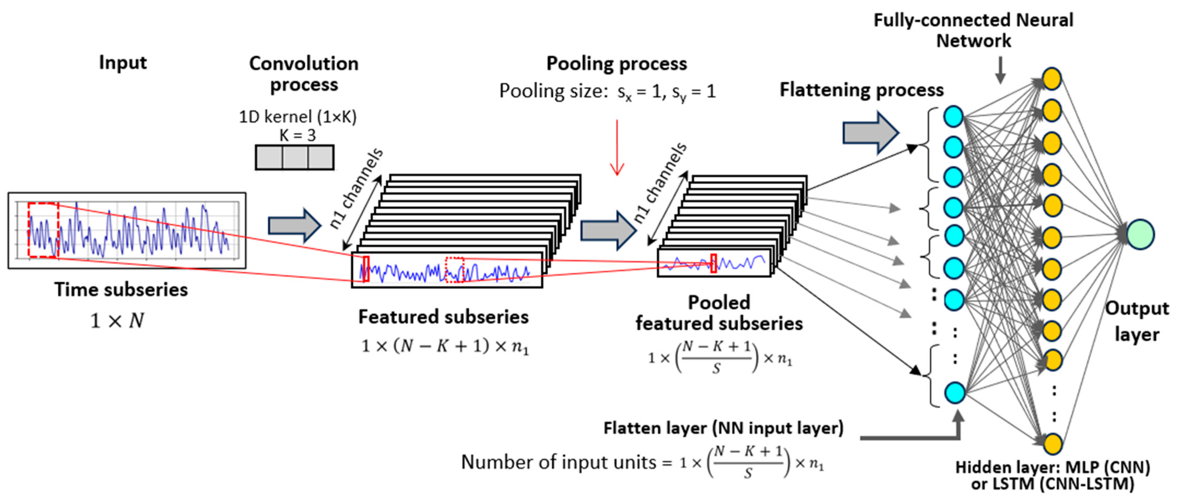
2.4.4. Convolutional Neural Network (CNN)
The CNN algorithm is a neural network specialized in processing complex data. Although widely used in image processing, CNN’s algorithms have also shown excellent results in time series simulation [
51]. In addition to the conventional MLP algorithm, the CNN algorithm includes a convolution and pooling layer, which makes it a powerful algorithm [
52].
In contrast to the LSTM, which considers past information in a sequence-based context window, the CNN considers past information through a context window that represents the spatial relationships between values in the feature map. As a result, the convolutional layers of the CNN can scan the input feature map and identify local patterns, using this past information to construct a representation of the input.
CNN differs from the LSTM by considering past information via a spatial context window instead of a sequential one. Thus, the convolution process in the CNN scans the input feature map and identifies local patterns, forming a representation of the input by utilizing this past information.
In the context of 1D CNNs, time series are processed as one-dimensional data (
) with a dedicated 1D kernel (
) and multiple channels (
) for diverse kernel training. Post-convolution, pooling shrinks the series size, optimizing computational efficiency. Subsequently, the resulting series is flattened to extract a single node for each value within the generated series. Preserving both time and channel dimensions, this methodology transforms time series into a format conducive to comprehensive feature extraction and analysis within the 1D CNN framework, preserving both the time and channel dimensions. Thus, the flattening process determines the neural network’s input nodes, computed as the product of the length of the grouped series and the number of channels, expressed as
. The fully connected MLP layer utilizes the flattened data to produce the final Output (
Figure 5).
The gradient descent optimization algorithm is used to update the parameters (weights and biases) of the CNN during training to minimize the loss between the predicted and actual output for the training samples [
53]. The CNN hyperparameters underwent a two-step manual tuning process using GridSearchCV. In the initial step, various hyperparameters were explored, including the number of neurons (50 to 400), activation functions (Relu, Tanh, and Sigmoid), optimizers (Adam and Adamax), learning rates (0.001 to 0.01), batch sizes (16, 32, 64), epoch numbers from 100 to 500 with early stopping set at 20. Regarding convolution, considerations encompassed kernel sizes of 3 and 5, number of filters of 8 and 16, “same” padding for maintaining subsequent length, strides of 1 and 2, and pool sizes of 1 and 2. In the second step, the evaluation extended to one and two hidden layers, with dropout rates ranging from 0 to 0.2. Hyperparameter optimization prioritized minimizing error and model complexity. The optimized values are detailed in
Table 2.
2.4.5. The Hybrid CNN-LSTM Algorithm
The hybrid CNN-LSTM algorithm, useful for tasks involving sequential data such as time series forecasting, combines the strengths of both the CNN and LSTM networks. Here, the CNN layer is typically used to extract high-level features from the input sequence. These features are then passed to the LSTM layer, which is responsible for modeling the temporal dependencies between the features and producing the final output [
54].
The key advantage of the hybrid CNN-LSTM algorithm is that it can effectively capture both local and global dependencies in the input sequence [
31]. The CNN layer is able to capture local patterns and features within the sequence, while the LSTM layer is able to model longer-term dependencies between these features. In addition, the hybrid CNN-LSTM algorithm that typically trains end-to-end using backpropagation allows the model to learn both the feature extraction and temporal modeling stages together, resulting in improved performance as compared to traditional methods that use separate feature extraction and modeling stages [
55]. Overall, the hybrid CNN-LSTM algorithm is a powerful tool for modeling complex sequential data and has been successfully applied in a wide range of applications.
The convolution process by which the CNN-LSTM algorithm architecture incorporates a LSTM network layer into the CNN algorithm architecture is illustrated in
Figure 5. CNN-LSTM hyperparameters were tuned in two steps with GridSearchCV, following a similar approach to CNN. They were optimized within the same ranges as CNN, seeking to reduce error and model complexity. Optimized hyperparameters are in
Table 2.
2.4.6. Seasonal Autoregressive Integrated Moving Average (SARIMA)
The SARIMA model is an extended statistical technique of the ARIMA model that is widely used to analyze and forecast time series data that exhibit seasonal behavior. The SARIMA model consists of six parameters
that are used to estimate the future value of a variable as a linear function of past observations and random errors. The first three parameters
represent the non-seasonal components of the model and are identical to those in the ARIMA model. The last three parameters
represent the seasonal components of the model and are used to model the seasonal behavior in the data. As proposed in past studies [
56], the method for creating the time series is as follows:
where
is the actual value (predicted value) and
is the random error (non-stationary time series), both at time
.
and
are the nonseasonal autoregressive and moving average components of order p and q, respectively.
and
are the seasonal autoregressive and moving average components of order
P and
Q, respectively.
and
are the non-seasonal and seasonal difference components.
is the backshift operator. The aboveground biomass time series in this study is a 15-day time step, hence the seasonal period is
. The SARIMA model is estimated using the Box-Jenkins methodology, which involves identifying the optimal values of the model parameters based on Akaike Information Criterion (AIC) statistical test. The SARIMA model parameters are shown in
Table 3.
2.5. Model Performance Evaluation
The model’s efficiency was assessed using the Root Mean Square Error (
RMSE) as follows:
where
is the observed time series value at time
i,
is the estimated/forecast time series value at time
i, and
is the number of time series data. RMSE values vary from 0 to
, using the same units as the variable being measured, with 0 indicating a perfect model with zero prediction error.
In addition, the model’s performance in percentage terms was assessed using the Mean Absolute Percentage Error (
MAPE):
MAPE values vary from 0% to , with lower values indicating more accurate predictions and 0% being a perfect model with zero prediction error. MAPE values less than 5% suggest an acceptable level of forecast accuracy, while values between 10% and 25% indicate low but acceptable accuracy, and values greater than 25% indicate an unreliable model. On the Relationship among Values of the Same Summary Measure of Error).
Moreover, model error was assessed using the Symmetric Mean Absolute Percentage (
SMAPE):
Unlike the mean absolute percentage error, SMAPE has defined limits. The formula mentioned yields outcomes ranging from 0% to 200%. SMAPE’s bounded nature improves forecast accuracy assessment by constraining extreme values for clearer error interpretation.
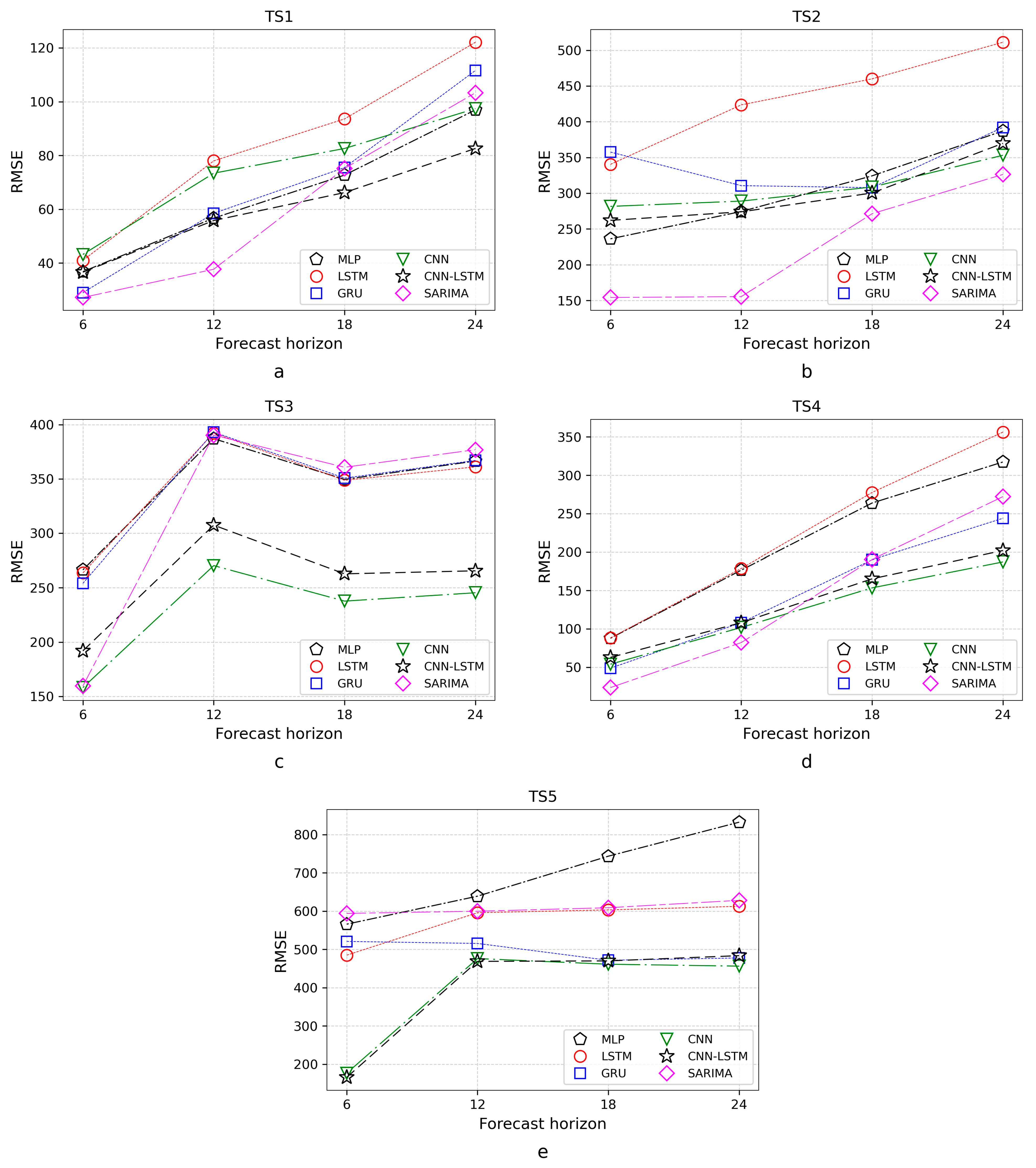
Furthermore, to rigorously compare RMSE values across distinct DL algorithms and cases, we conducted the Analysis of Variance (ANOVA) statistical test. This method revealed significant variations in RMSE outcomes, enhancing our understanding of relative efficacy. Within each case, we compared average RMSEs from twenty-five replications using the CNN-LSTM algorithm with those from other DL algorithms, providing insights into its performance against counterparts.
4. Discussion
The first finding of this study is that the CNN-LSTM hybrid model did not exhibit absolute superiority over other DL models or the statistical model in predicting vegetation biomass. This might suggest that the CNN-LSTM model did not have a significant advantage over the other models in accurately predicting vegetation biomass within the constraints of a limited dataset. Even though none of the models evaluated demonstrated complete dominance, the SARIMA, CNN, and CNN-LSTM models exhibited better performance compared to the other three models included in this study. Contrary to numerous studies that claim the supremacy of DL models over classical statistical approaches, this study shows that statistical models could still provide better or comparable predictions than sophisticated models.
Several recent studies have reached similar findings. For instance, [
19] found that basic statistical models performed better than machine learning (ML) models and indicated that complex models are not necessarily superior to simple forecasting models [
19]. Other research has demonstrated the superiority in predictive capabilities of statistical models over ML models with respect to energy production [
38], financial market data [
57], health, and cryptocurrency [
58].
The disappointing performances of the DL models might be related to specific characteristics of time series data, such as periodicity, seasonality, and noise [
19,
21,
38], along with factors such as the dataset size [
19,
37] and model parameters [
58]. Since ML models involve multiple nonlinear transformations, it would seem that they should prove superior to statistical models; however, evidence from previous studies has indicated that ML models cannot be generalized from small datasets—a limitation relative to traditional statistics.
Although both statistical models and DL models rely on data to make predictions, ARIMA models concentrate on predicting future values based on past neighboring and seasonally lagged data, while DL models employ sliding window data that undergoes several optimized transformations during the model training process. When time series data is limited in size, it may be insufficient to determine the optimal transformations and identify the key predictor neighbors for accurate forecasting; consequently, model efficiency may be compromised. Furthermore, the presence of noise and chaos in the time series can add to the challenge of identifying the optimal transformations [
57]. Likewise, the prevailing conditions of intense drought during the last two years of the analyzed biomass time series could be exerting a notable impact on the results of near-future forecasts through ARIMA models and neural networks. The ARIMA model’s predictive accuracy, for example, is largely dependent on historical patterns and trends. Given the extended period of arid conditions, the model might overemphasize the significance of these dry years in its predictions. Consequently, it could be producing forecasts that underestimate the potential for variance, especially if the future is anticipated to be less drought-prone. The performance of the deep learning algorithms may also have been hampered by a lack of wet periods in the previous two years. Thus, the model might be struggling to generalize effectively from such a narrow range of variation, potentially resulting in overly optimistic or pessimistic predictions.
Cerqueira et al. similarly found that the ARIMA models are better than the ML models when time series data is limited in size; their experiments considered a time series of 1000 values [
37]. Other studies, such as that of Makridakis et al., have obtained similar results for time series of between 1600 and 1800 values [
19]. Similarly, Vabalas et al. showed limitations in the performance of ML models based on a limited sample size [
59]. These studies are consistent with the findings of our study, which considered just 496 values with seasonality. This logic is consistent with the fundamental principles of DL algorithms, indicating that the size of the training dataset has a direct impact on their performance. A larger and more diverse dataset enables algorithms to generalize and produce more accurate predictions, whereas a small dataset may result in overfitting and poor performance on new data [
19,
42].
Additionally, this study found that, as with the other DL and statistical models, the forecast accuracy of the CNN-LSTM model typically diminished as the forecast horizon increased. However, this relationship was not always monotonic, meaning that the decrease in forecast accuracy was not consistent throughout the forecast horizon. There could be instances where the accuracy of the forecast might increase, decrease, or stay the same as the forecast horizon changes. The reason behind this non-monotonic relationship could be due to several factors, including noise or underlying patterns in the data and the type of forecasting model used. This is consistent with the results obtained, for example, by Zhang, who employed SVR and found a non-monotonic relationship between MSE and the forecast horizon in iterative forecasting. The iterative prediction approach, despite being simple and practical, suffers from low performance over long periods due to the accumulation of errors. The errors found in each step are included in the forecast of the next step as we feed the model [
19]. Although DL methods are sophisticated, the uncertainty characteristics of vegetation biomass will lead to forecast errors and the propagation of errors in an iterative forecast over a long horizon. In this regard, further exploration of DL models that include non-iterative processes is required. These results underscore the dynamic nature of vegetation biomass production across time scales. Climatic dynamics, including precipitation changes, temperature fluctuations, and other growth-influencing factors, might lead to varying predictability. DL models could be capturing these complexities, explaining the non-monotonic forecast accuracy with changing horizons. This highlights the need for further research to delve into these intricate relationships and their impact on vegetation biomass fluctuations.
Finally, while sophisticated methods such as hybrid models have demonstrated outstanding effectiveness in a variety of fields, this study did not replicate such results, instead highlighting statistical models for forecasting vegetation biomass. The time series evaluated in this study exhibit specific characteristics, and thus, the findings of this study are limited to time series with these characteristics. In this sense, more studies on time series forecasting using modern forecasting techniques for limited data sizes are clearly required.
5. Conclusions
This study assessed the effectiveness of DL models, including the hybrid CNN-LSTM, for predicting aboveground vegetation biomass time series with limited size data, comparing their performance to the traditional SARIMA statistical model, which served as a benchmark for evaluation. To conduct this assessment, we utilized five aboveground vegetation biomass time series datasets, consisting of values collected at 15-day intervals over a 20-year period from fields in Kenya. The outcomes of our study demonstrated significant differences in the forecasting accuracy of the various models. The CNN-LSTM model was not significantly more accurate than the other models; however, it did rank alongside the SARIMA and CNN models as one of the three most reliable—with the statistical model, SARIMA, slightly outperforming the other two. The LSTM and MLP were the least accurate models. The moderate performance of the hybrid CNN-LSTM model could be attributed to the specific characteristics of the data, as well as the limited size of the vegetation biomass time series. These factors may have restricted the learning capacity of the model in spite of its sophisticated prediction architecture. It is possible that the performance of the proposed model could improve as larger quantities of aboveground vegetation biomass data are collected in the future.
Furthermore, this study revealed that the accuracy of the hybrid CNN-LSTM model—as well as the other models—differed significantly depending on the forecast horizon. As the prediction horizon increased, the accuracy of the models tended to decrease, resulting in larger forecast errors. Although there was a clear overall trend, the relationship between forecast horizon and model accuracy was not strictly monotonic. Consistent with prior research, the decline in model performance over longer forecast horizons could be attributed to the cumulative error that occurs in the iterative prediction process.
Findings from this study may not be generalizable to other vegetation biomass time series data with different characteristics and sample sizes. Meanwhile, based on our outcomes, it is evident that with the limited size and specific characteristics of aboveground vegetation biomass time series, there is no guarantee that machine learning forecasting techniques will outperform statistical methods. Moving forward, it would be beneficial for future research to explore the application of more advanced machine learning models on larger vegetation biomass time series datasets, including but not limited to algorithms such as naive Bayes, gradient boosting algorithms, and Generative Adversarial Networks (GANs). The inclusion of these advanced models could shed further light on their efficacy in comparison to traditional statistical methods. For shorter time series, we recommend continued evaluation of various methods to achieve acceptable levels of accuracy. Moreover, future studies should explore diverse parameters unexplored here, such as the input window length, which could significantly impact forecasting accuracy.


