Article

Evaluating the Topographic Factors for Land Suitability Mapping of Specialty Crops in Southern Ontario

Department of Geography, Environment & Geomatics, University of Guelph, 50 Stone Road East, Guelph, ON N1G 2W1, Canada
*
Author to whom correspondence should be addressed.
This paper is a part of the Master Thesis of Laura Lisso, presented at The University of Guelph, Canada.
Agronomy 2024, 14(2), 319; https://doi.org/10.3390/agronomy14020319
Submission received: 12 November 2023 / Revised: 26 January 2024 / Accepted: 26 January 2024 / Published: 1 February 2024

Abstract

:
Climate change research identifies risks to agriculture that will impact agricultural land suitability. To mitigate these impacts, agricultural growing regions will need to adapt, diversify, or shift in location. Various machine learning algorithms have successfully modelled agricultural land suitability globally, predominantly using climate and soil features. Topography controls many of the environmental processes that impact agriculture, including soils, hydrology, and nutrient availability. This research evaluated the relationship between specialty crops and topography using land-surface parameters extracted from a 30 m DEM, soil features, and specialty crop presence/absence data derived from eight years of previous land classifications in southern Ontario, Canada. Using random forest, a model was developed for each specialty crop where feature permutation importance, Matthew’s correlation coefficient, and the area under the precision-recall curve was calculated. Elevation relative to watershed minimum and maximum, direct radiation on Day 172, and spherical standard deviation of normals were identified as the mean most important topographic features across all models and beet crops were found to have the highest association with topographic features. These results identify locations of agricultural expansion opportunities if climate becomes more favourable. The importance of topography in addition to climate and soils when identifying suitable areas for specialty crops is also highlighted.

1. Introduction

Climate change poses a risk to current agricultural distributions as climatic patterns alter across landscapes [1,2,3,4,5]. Changes in soil fertility, temperature, number of growing days, and water availability cause stress on crops that reduce quality and yield [6]. These changes will particularly impact specialty crops and especially fruits and vegetables. Specialty crops are inherently higher risk and will require a response to the impacts of climate change sooner than more resilient field crops [7,8,9,10,11,12,13]. Adapting, diversifying, and shifting growing regions to follow these changes is a way to improve the resilience of agriculture and its resulting food security over time [4]. While it is crucial to ensure the present and future climate of an area is well-suited to growing a particular crop, it is also imperative to ensure the land is also suitable.
Soils of land areas are well-studied in relation to agricultural land suitability, ensuring adequate nutrients, moisture, and soil type [7,11,14,15]. However, topography is less well studied in relation to agricultural land suitability. Topography can describe important information about the landscape because hydrology, soils, erosion, nutrient availability, and radiation are influenced by an area’s topographic properties [16,17,18,19,20]. Land-surface parameters (LSPs) can be extracted from a digital elevation model (DEM) to represent these various aspects of topography that describe the surface shape, movement of materials, microclimates, and more [21,22,23,24]. There is currently a limited inclusion of LSPs in agricultural suitability modelling despite their direct influence on the environmental phenomena that impact the viability of land to grow particular crops. Understanding these impacts can improve methods of agricultural modelling across larger, heterogenous landscapes [19,25,26,27,28].
Identifying suitable areas for agriculture is commonly accomplished using machine learning based analysis methods [9,11,15,29,30,31,32,33,34,35,36,37]. Species presence/absence samples are often used as the training data for these models, as each species can exist in a spatial extent with unique combinations of environmental gradients [11,29,36,38,39]. Environmental features (sometimes known as covariates) are the representations of these environmental gradients for the purpose of input into a machine learning algorithm. These algorithms have displayed promising results with high levels of accuracy, particularly when using the random forest algorithm [29,36,40,41].
There is currently limited research focused on the land suitability for specialty crops in temperate regions despite their heavy economic input requirements (and potential return) as well as their importance to food security in the face of climate change [2,6,12,15,29,36,37]. The incorporation of topographic information into the modelling techniques that have already been established in the field may help to identify ways to improve future agricultural planning under multiple climate change scenarios. The objective of this research is to evaluate the relationship between topography and the location of specialty crops in southern Ontario. This was evaluated using past distributions of specialty crops derived from the eight most recent years of Agriculture and Agri-Food Canada’s (AAFC) Annual Crop Inventory (ACI) as training data and by deriving a selection of environmental features for input into a random forest algorithm. This research uses multiple LSPs, including some more recent parameters, that have not yet been evaluated in relation to the land suitability of specialty crops in previous studies.

2. Materials and Methods

2.1. Study Area

A region covering much of southern Ontario was used as the study area for this research, based on the extent of the classification of all agricultural classes in the ACI from 2014 to 2021 (Figure 1). The study area encompasses 95.1% of the Province’s fruit crops and 97.1% of the Province’s vegetable crops at 187 km2 and 502 km2 respectively [42]. The study area spans 71,500 km2 and covers a wide range of climatic, topographic, and soil characteristics. With this variation, specialty crops are produced in specific areas of the study area, such as grapes and tender fruit along Lake Ontario in the Niagara Region, tomatoes near Leamington in Essex County, and various vegetables in the municipality of Chatham-Kent and the Holland Marsh [43]. The study area includes areas of plant hardiness zone classifications from 4b to 7a, corresponding to minimum plant survival temperature ranges of −31.7 °C to −28.9 °C and −17.8 °C to −15 °C, respectively [44]. The topography of the area is overall low-relief and characterized by rolling hills, with minimum and maximum elevations of 52.0 m and 541.4 m respectively (Figure 1). A large portion of the soils covering this area are grey-brown luvisols [45].

2.2. Annual Crop Inventory Assessment

The ACI was used to derive presence/absence data for each specialty crop type in the classification. The ACI classifies land use yearly into a 30 m grid cell size raster by collecting presence data collected through field work and remote sensing techniques into a random forest model [46]. General classifications exist for water, urban, wetlands, and forests (e.g., coniferous, deciduous, and mixed). However, the focus of the ACI is on agricultural classes, of which 56 of the 72 total classes are categorized as agricultural. Of those 56 classes, 24 are specialty crops, which includes fruits, vegetables, ginseng, tobacco, hops, and nursery crops. Based on the risk level identified in previous research, this research focused on the fruit and vegetable classes in the ACI, of which there were 13—four vegetable classes and seven fruit classes.
The ACI has been produced annually for southern Ontario since 2011, however this research only used data from the years 2014 to 2021 as sub-classes of fruit and vegetable crops were not yet identified in the ACI from 2011 to 2013 [43,47,48,49,50,51,52,53]. This land was instead classified as undifferentiated agriculture. From 2014 to 2021, the ACI classified the following fruit and vegetable classes; tomatoes, potatoes, beets, other vegetables without their own unique category (e.g., brassicas, leafy greens, and legumes), berries with subclasses blueberries, cranberries, and other berries (e.g., raspberries and strawberries), orchards, vineyards, and other fruit without their own unique category (e.g., melons). The following fruit classes were combined into one group titled “berries and other fruit” due to low classified presence across the study area and some classes being introduced after 2014: berries, blueberries, cranberries, other berries, and other fruit. As a result, all other classes remained independent.
Each specialty crop class was extracted from the ACI for each year from 2014 to 2021. An eight-year range of classifications from the ACI was used to account for any crop rotation patterns that could have removed grid cells of a vegetable classifications for a single or small range of years, as well as the case that some specialty crop locations were insufficiently classified. User accuracies ranged from 26.1% to 100.0% for most crops each year, but some crops had lower user accuracies such as beets in 2016, blueberries in 2018, and cranberries in 2020, where the user accuracy for each was 0.0% (Table 1). To ensure an accurate dataset, a presence/absence classification layer was created for each specialty crop using classification years where user accuracies (Table 1) were greater than 60.0%, 70.0%, and 80.0%. This resulted in a total 15 presence/absence layers based on the accuracy thresholds, for beets (70, 80), berries and other fruit (60, 80), orchards (70, 80), other vegetables (70, 80), potatoes (60, 70, 80), tomatoes (60, 80), vineyards (70, 80). In the discussion below the presence/absence layers will be denoted along with the accuracy, for example, vineyard_70 is used to describe the vineyard presence/absence layer at the 70% user accuracy level. For each of the 15 presence/absence layers, grid cells classified for two or more years were considered as sufficient evidence for presence of that specialty crop layer, this step was included to account for misclassifications in the ACI.

2.3. Features

A total of 34 features were derived for input into the random forest model (Table 2). Of those, 27 features described topographic properties while the remaining seven features described soil properties. The topographic features were derived from a 30 m grid cell size provincial DEM from the Ontario Ministry of Natural Resources and Forestry [54] from which a variety of LSPs were extracted. The DEM was pre-processed depending on the type of LSP that was extracted, such as hydrologically conditioning a DEM by filling pits, breaching depressions, and fixing flats for extracting hydrological LSPs such as calculating contributing area and the topographic wetness index [55]. Other pre-processing methods applied were the feature-preserving DEM smoothing (FPDEMS) algorithm with various filter sizes, and a Gaussian filter with a sigma of 0.75. The preprocessing techniques and filter size applied to the LSPs are listed in Table 2. The soil features were derived from the Ontario Soil Survey Complex, a vector polygon dataset at a scale of 1:20,000 [56] as well as the Detailed Soil Survey dataset, a vector polygon dataset at a scale of 1:50,000 [57]. Both vector polygon layers were converted to 30 m grid cell size raster layers to match the DEM. Water and urban areas were masked from all feature layers to ensure predicted suitable areas were only being identified on developable land.
LSPs were selected based on their ability to describe the environmental conditions affecting agriculture such as water availability, climate, soil properties, elevation, and slope. The LSPs extracted from the DEM describe six categories of topographic variables, including measures of surface shape, topographic roughness and complexity, upslope area or flow accumulation, topographic position, visual exposure and landscape visibility, and insolation [22,24,58]. Measures of surface shape such as curvatures influence deposition, erosion, and flow convergence/divergence processes which in turn impacts soil development [58,59,60,61,62,63,64,65]. Topographic roughness (consisting of both ruggedness and complexity) describes elevation variation in an area and provides insight into geologic structures and their formation, which can influence soil properties and erosion potential [58,66,67]. Upslope area or flow accumulation LSPs describe the saturation and overland flow potential and location for a landscape based on the surrounding elevations [58,68,69,70,71,72]. Topographic position describes how elevated or low-lying a site is relative to its local neighbourhood, which describes the drainage ability, exposure/visibility, and microclimate [58,73,74]. Visual exposure and landscape visibility describes the exposure of an area to wind and other elements, which influences an area’s microclimate [58,75]. Insolation describes climatic properties of an area, specifically related to radiation and daylight [58,76,77].
To reduce noise and remove unwanted artefacts from the DEM, smoothing methods were applied dependent on the desired LSP to be extracted. As the DEM represents the study area at a more moderate scale with a 30 m grid cell size, only conservative smoothing techniques were applied. This was largely accomplished using Lindsay et al.’s [78] FPDEMS algorithm, which smooths roughness while preserving edges important to topography such as breaks in slope. The filter size for each LSP varied dependent on the amount of smoothing required to remove artefacts but preserve the relevant topographic features. For LSPs more sensitive to noise, surface roughness, and anthropogenic off-terrain objects such as curvatures [64,79], a larger filter size was applied to reduce the prevalence of these artefacts.
For upslope area/flow accumulation LSPs, hydrological conditioning was applied to a smoothed DEM. The FPDEMS was selected as it has been shown to preserve drainage features better than a mean, median, or gaussian filter [78,80]. To enforce flow paths through roads, the breach depressions least cost algorithm from WhiteboxTools was used as it alters the fewest number of grid cells and works well in the presence of roads [81]. This algorithm also adjusts flat areas to have a small slope to enforce flow and fills any remaining pits and/or depressions that could impede flow paths.
For roughness related LSPs, roughness appears at a smaller scale than landscape features, but anthropogenic features still need to be removed from the DEM, thus a different smoothing approach was applied. To remove noise and off-terrain objects mimicking roughness such as vegetation canopies but preserve roughness, a Gaussian filter was applied to the DEM for these LSPs, with a sigma of 0.75.

2.4. Presence/Absence Data Sampling

Up to 2200 samples from each presence/absence specialty crop layer were collected for use as training data within a random forest model. To obtain the samples, the conditioned Latin hypercube sampling (cLHS) method in WhiteboxTools, based on Minasny and McBratney’s [82] algorithm, was used in combination with a stratified sampling method from the R package “raster”. The stratified sampling method sampled both presence and absence sites from each of the 15 presence/absence layers. The cLHS method is common in digital soil mapping as it selects sample sites that cover the full range of values for every environmental feature input [82] and was thus primarily used to ensure adequate sample sites were selected for each continuous feature. While the study area covers more than 79 million grid cells, the presence locations of crop classes cover a much smaller land area, covering a range between 1961 to 140,610 grid cells, depending on crop class and user accuracy. As a result, most sample sites collected through the cLHS method were classified as absence data. Thus, combining the two sampling methods was necessary to obtain an adequate number of both crop presence and absence samples.
Up to 1400 absence sample sites were identified for each specialty crop accuracy class, with up to 800 points from the stratified sampling method and up to 600 from the cLHS method. Up to 800 presence sample sites were identified for each crop-accuracy class, with nearly all sites obtained from the stratified sampling method. An insufficient number of presence points for berries_other_fruit_60, berries_other_fruit_80, and other_veg_80 was captured (5, 2, and 0 respectively) therefore, these layers were removed from further analysis. This resulted in 12 sample layers that were used for the analysis, i.e., beet_70, beet_80, orchard_70, orchard_80, other_veg_70, potato_60, potato_70, potato_80, tomato_60, tomato_80, vineyard_70, and vineyard_80. Each model was run with a decreasing number of sample sites, where the difference in classified proportions was then calculated. The variance in results was insignificant until the sample size for each layer was reduced by 50%, indicating sufficient sample sizes for all layers.

2.5. Random Forest Models

Machine learning algorithms are widely applied to modelling agricultural distributions and predicting agricultural land suitability [11,29,36,41]. Random forest is frequently used in agricultural modelling as it can effectively handle a large amount of data and is less sensitive to outliers [29,33,34,36]. Random forest is an ensemble bagging method machine learning algorithm that creates many decision trees [83]. A subset of randomly selected features is then put through each tree and the result is selected based on the most predicted class of the trees for each grid cell.
A random forest algorithm was trained for each of the 12 target specialty crop layers using the fitting method “rf” from the R package “caret”, which accesses Breiman’s [83] “randomForest” package. The sample sites collected through the stratified sampling method and the cLHS sampling method were used as the training/validation data, while the 34 features were used as the predictor layers. A repeated k-fold cross validation resampling method was used to split each dataset into training and test sets internally with 10 folds repeated five times. This method reduces model overfitting as all the available data is used as both the training and test dataset [84,85]. For the fitting method “rf”, the tuning parameter “mtry” determines the number of features randomly sampled at each node split in the decision trees [83]. This tuning parameter was assessed during the training of each model for values 1 to 34 (i.e., the number of features), with the value used for prediction being selected based on the highest Cohen’s Kappa Index. The selected value for this parameter varied across all 12 models. Trials of the models were run with 250, 500, 750, 1000, 1250, and 1500 trees. The amount of presence/absence classification error was low for all models run with 1000, 1250, and 1500 trees, but there was no significant decrease in error for 1250 and 1500 trees. Thus, 1000 trees were used in all 12 final models.
The accuracy of the model was evaluated using Matthew’s correlation coefficient (MCC) and the area under the precision-recall curve (AUC-PR). Both accuracy measures were calculated based on a confusion matrix using the values of true positives (TP), false positives (FP), true negatives (TN), and false negatives (FN), where positives represented presence data and negatives represented absence data. The MCC calculation:
M C C = T P × T N F P × F N ( T P + F P ) ( T P + F N ) ( T N + F P ) ( T N + F N ) ,
considers all four elements in a confusion matrix, providing a balanced accuracy measure where classes are considered to be equally important [86]. MCC values can range from negative one to positive one, with positive one indicating perfect agreement in classification, zero indicating no agreement, and negative one indicating perfect disagreement [86].
The AUC-PR score consists of two measures derived from the confusion matrix plotted against each other, precision:
P r e c i s i o n = T P T P + F P
plotted on the y-axis and recall:
R e c a l l = T P T P + F N
plotted on the x-axis, and the area under the resulting curve calculated [87]. Precision accounts for TP and FP, while recall accounts for TP and FN, but TN values are not accounted for in either measure, thus the AUC-PR primarily measures the accuracy of presence locations. AUC-PR values can range from zero to one, with higher AUC-PR values representing a higher level of agreement and lower AUC-PR values a lower level of agreement [87]. MCC and AUC-PR are both more robust than other accuracy measures when the class samples are imbalanced and are recommended for binary classifications [86,87]. The class samples were imbalanced in favour of absence data for all specialty crop layers as the areas for crop presence were much smaller than areas of absence.
Feature importance was calculated during the training of the model using the feature permutation importance measure, which shuffles each feature in the training dataset and calculates the difference between the accuracies, normalized by the standard error [83]. The feature importance values were then scaled to 100. The final trained model was then applied to the entire study area using the full range of the input features to produce a binary raster layer predicting suitable and unsuitable land for growing each specialty crop layer across the study area.

3. Results

3.1. Model Accuracies

The MCC for the training set of each specialty crop model ranged from 0.79 to 0.94 (Table 3), with a mean value of 0.87. Vineyard_80 had the highest MCC of 0.94, with the lower user accuracy vineyard layer, vineyard_70, having a similarly high MCC of 0.92. The lowest MCC was for orchard_70 and potato_80 (0.79). Orchard_80 had a similar MCC while potato_60 and potato_70 had higher MCC values of 0.88 and 0.87 respectively. The MCC was consistently similar between the different user accuracies for specialty crop types, except for potatoes. The higher user accuracy (>80%) for both beets and potatoes had a lower MCC than the lower accuracy (>60% and >70%) crop models. This difference was smaller for beets, with a difference in MCC of 0.05 but higher for potatoes, with the greatest difference being 0.09 between potato_80 and potato_60.
The AUC-PR for the training set of each specialty crop accuracy model ranged from 0.86 to 0.98 (Table 3), with a mean value of 0.92. The highest AUC-PR belonged to vineyard_70 and vineyard_80 with a value of 0.98. The lowest AUC-PR belonged to other_veg_70 (0.86). The AUC-PR was similar if not identical for most crop types regardless of user accuracy value with the exception of beets. Similar to the MCC values, the higher user accuracy (>80%) for beets had a lower AUC-PR (0.93) than the lower accuracy (>70%) beets model (0.96).

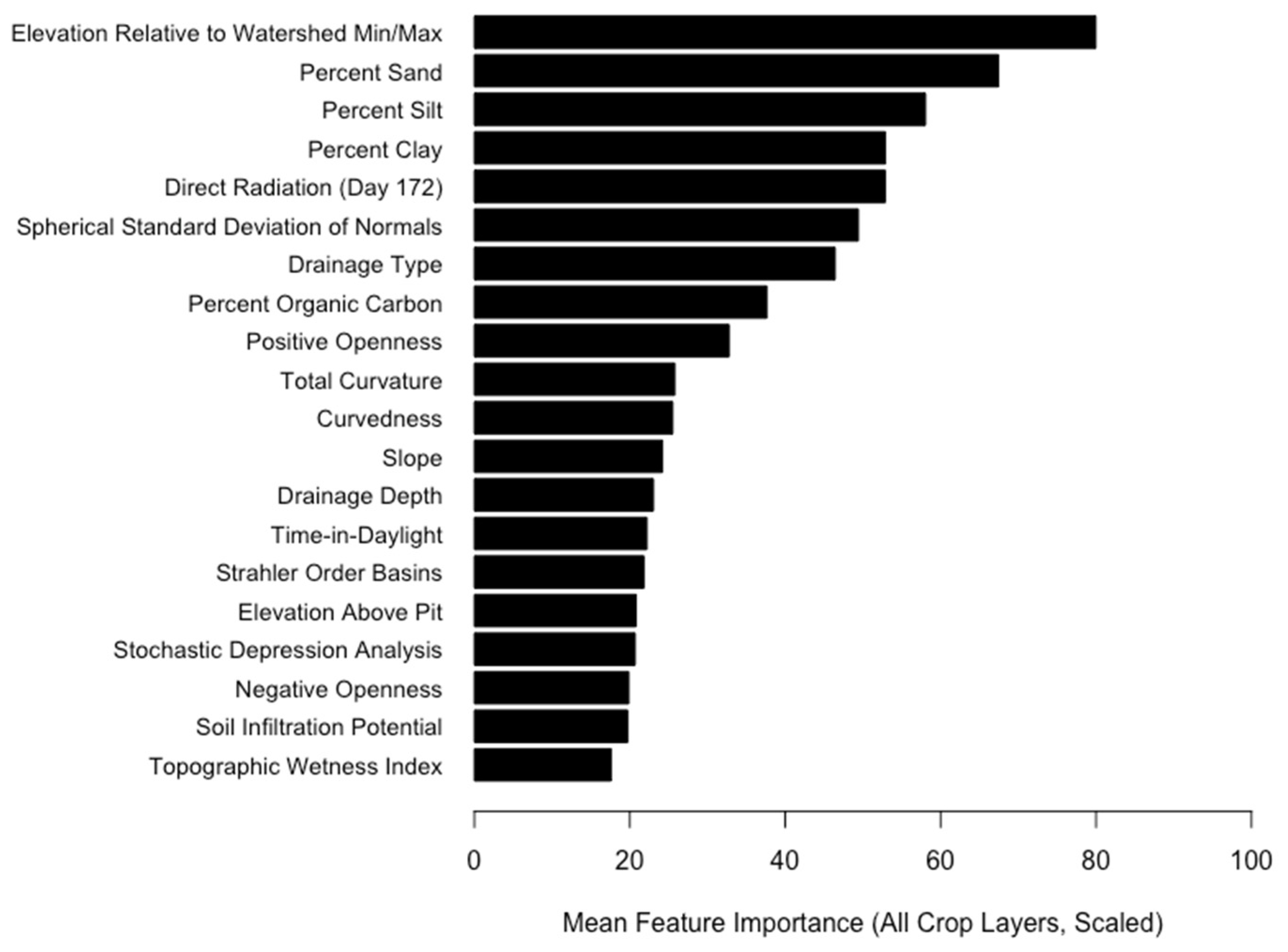
3.2. Feature Importance

On average, of the 34 features input into the models, the most important topographic features were elevation relative to watershed minimum and maximum, direct radiation on Day 172, and spherical standard deviation of normals, which had mean importance across all models of 80.0, 52.9, and 49.4 respectively (Figure 2). Other highly ranking topographic features across all models were positive openness, total curvature, curvedness, slope, time-in-daylight, Strahler order basins, elevation above pit, stochastic depression analysis, negative openness, and topographic wetness index, with the average importance values ranging from the highest at 32.8 to the lowest of the top 20 at 19.5.
As expected, all 7 soil features included in the models ranked highly in feature importance for each specialty crop model. Soil texture features ranked higher than other soil features, with percent sand ranking the highest mean across all models, while soil infiltration potential ranked the lowest.
The individual feature importance plots rank all 34 features for each crop layer [88]. The mean most important feature, elevation relative to watershed minimum and maximum, was found to be the most important overall feature for beet_70, beet_80, orchard_80, and potato_60. Elevation relative to watershed minimum and maximum was also the most important of the topographic features for orchard_70, potato_70, potato_80, tomato_60, and tomato_80, with at minimum a soil texture feature preceding. Only three crop layers were found to have a different topographic feature than elevation relative to watershed minimum and maximum as either the most important overall or the most important topographic feature, those being other_veg_70, vineyard_70, and vineyard_80. For other_veg_70, the most important topographic feature was spherical standard deviation of normals, preceded by drainage depth and percent silt. For both vineyard_70 and vineyard_80, direct radiation on Day 172 was the most important feature overall.
The feature importance results indicated that beets were the crop most associated with topographic features, with 80% of feature importance being attributed to topographic features in both beets_80 and beets_70. Topographic features also displayed a relatively high association with orchards, accounting for 68% and 63% of the feature importance for orchards_80 and orchards_70 respectively. Vineyards were also found to have a relatively high topographic feature importance, with 64% and 65% attributed importance for vineyard_70 and vineyard_80 respectively.

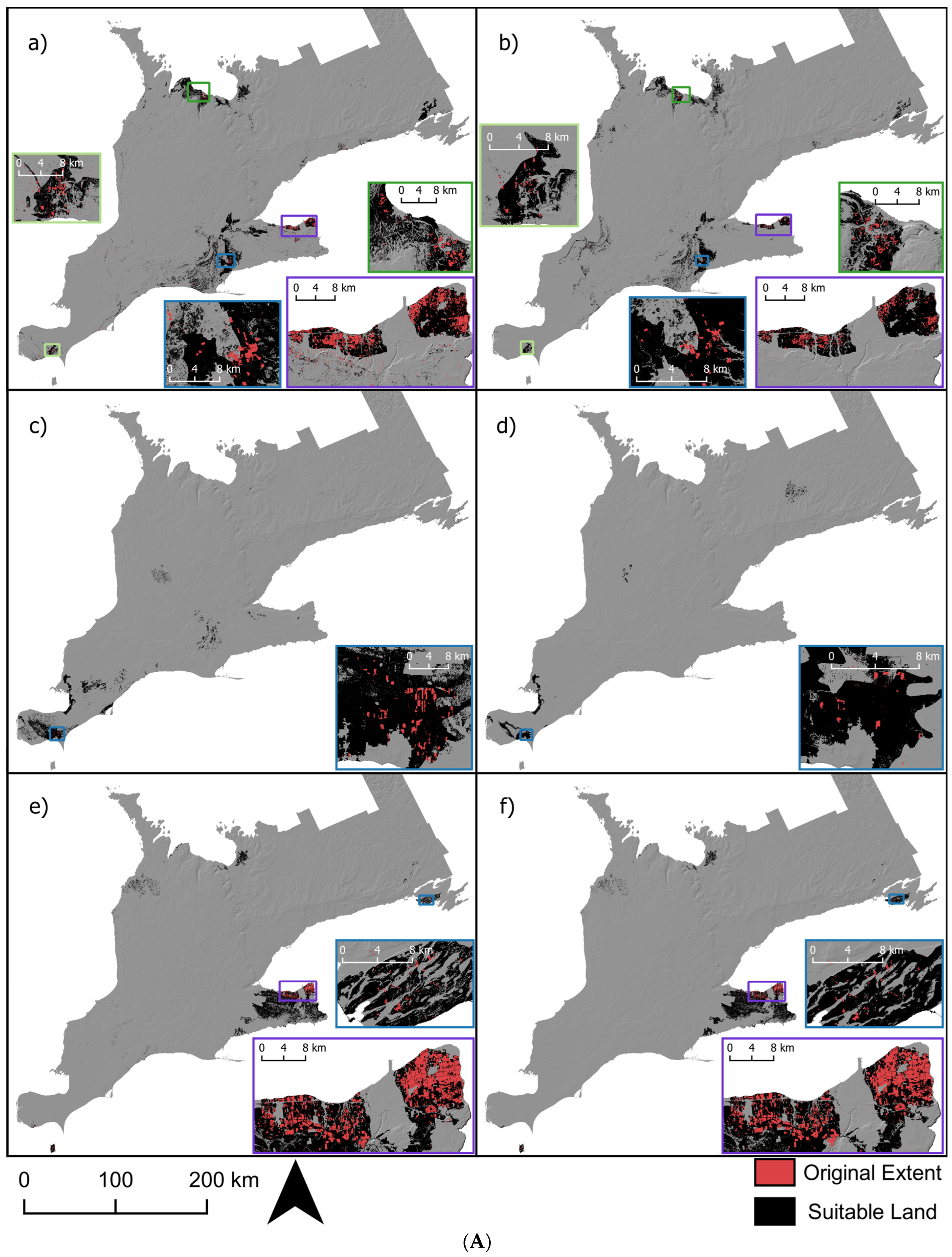
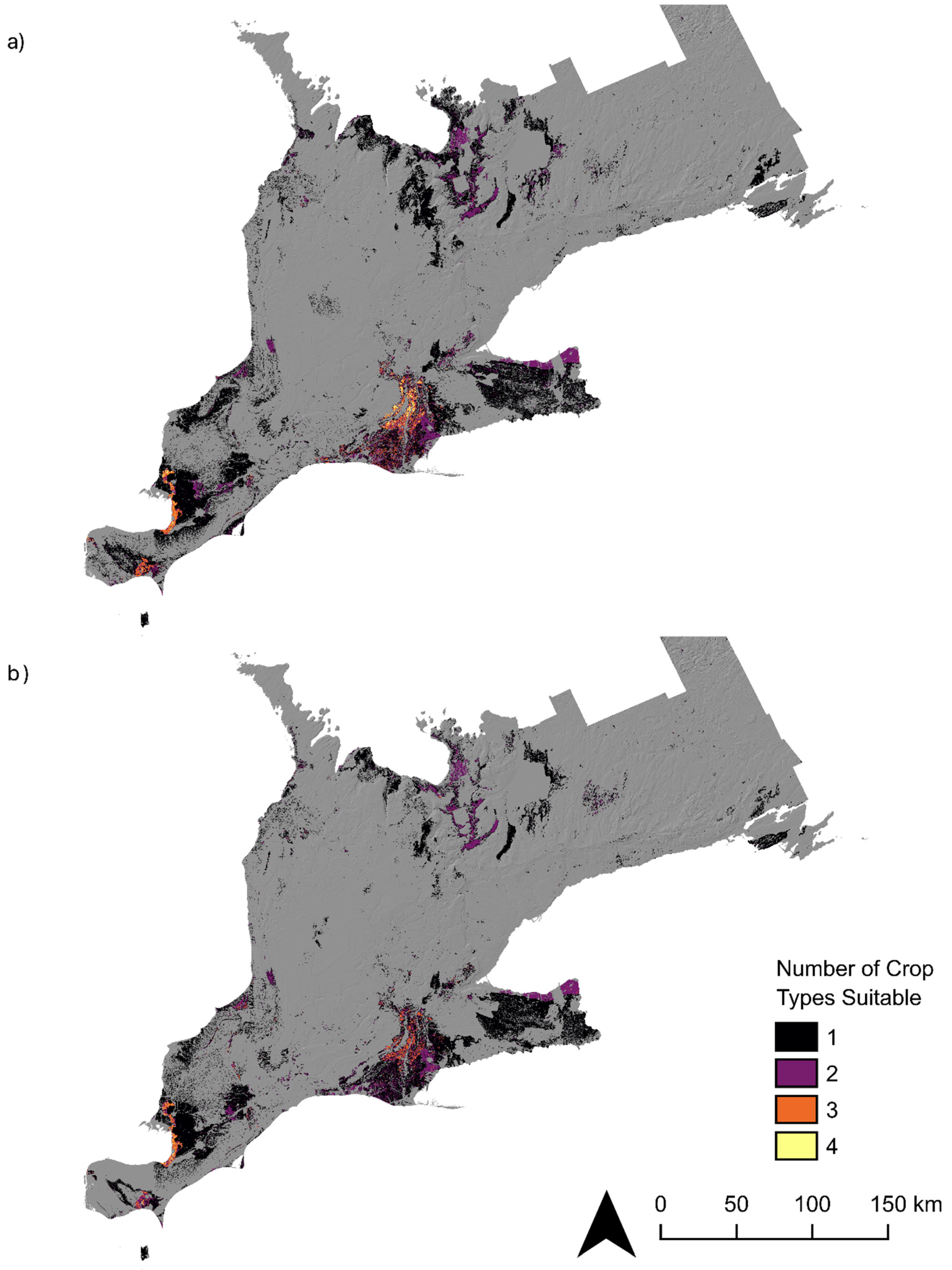
3.3. Crop Suitability

The results of each specialty crop model were mapped in comparison to their original extent from the presence/absence layers (Figure 3A,B). The original extents identified for each specialty crop type display where the crops are classified by the ACI at the same grid cell for two years or more over an eight-year period (2014 to 2021). These extents were inherently human-driven. All specialty crop suitability maps displayed areas of potential expansion from their original extent based on the predictions using topographic and soil features. Within specialty crop classes, the size of suitable areas decreased slightly as user accuracies increased for all specialty crop types. A similar pattern of suitability across the study area was still followed despite these decreases in size.
While areas overlapped between specialty crop classes, no specialty crop showed the same suitable distribution as another. Figure 4 displays maps of areas of suitable land overlap based on the lower user accuracies of the six crop types (>60% and >70%) and the higher user accuracies of the six crop types (>70% and >80%). For both the low and high user accuracy maps, the maximum number of crop types with suitable land classified at the same grid cell was four.

4. Discussion

This research explored the relationship between suitable growing regions of specialty crops and their topographic properties. The models were found to be moderately to highly accurate, with the lowest MCC equal to 0.79 and the lowest AUC-PR equal to 0.86 (Table 3). It was also found that the most important topographic features for the selected specialty crops were the elevation relative to watershed minimum and maximum, direct radiation on Day 172, and spherical standard deviation of normals. These features showed a stronger importance for specialty crop distributions (Figure 2) relative to the most used LSPs in other agricultural modelling research (i.e., slope, topographic wetness index, and aspect), which indicates the importance of including more topographic features in future modelling scenarios.
Beets were found to be the crop most associated with topography, with 80% of their feature importance being attributed to topographic features. This indicates that topography has the potential to encode important information about suitable distributions of specialty crops. However, the suitability of land for crop types is reliant on the presence locations identified, which are also influenced by factors outside of direct environmental conditions, namely anthropogenic influences. These factors include historical distributions, management practices such as resource input, crop rotation, and multiple cropping systems, and related land suitability between crop types [89,90]. On land that is suitable for multiple crop types, growers may prioritize more valuable crops and/or crops with less suitable land availability, impacting the extent of suitable land identified from presence/absence data. Land suitability, namely topography, may also not be considered extensively by growers, rather deciding on specialty crop locations based on climate conditions and other anthropogenic influences such as proximity to markets and production facilities [89]. These decisions could also exclude potential suitable topographic conditions from the current extent of specialty crops. These factors are not accounted for in the models, and thus the topographically suitable extent identified for specialty crops in this research is assumed to identify a larger extent than where these crops would actually be grown. However, this supports multiple planning options such as further filtering suitable areas for specialty crops based on future climate scenarios and/or economic decisions.

4.1. Suitable Areas for Specialty Crops

While no crop type has the same predicted distribution, some areas do overlap. The potential growth capability for multiple specialty crops in an area indicates a good expansion or adaptation opportunity, dependent on a climate evaluation. This way, the area can be diversified and/or focused on the population’s need, as well as ensuring a resilient agricultural system under varying climate conditions. The area beginning along the shores of Lake Erie in Norfolk County and expanding outwards has a great deal overlap between the following crop types: potatoes, other vegetables, orchards, and, to a lesser extent, tomatoes. Within the County of Chatham-Kent, particularly along the shore of Lake St. Clair and surrounding Leamington, there is another large overlap in the crop types potatoes, other vegetables, tomatoes, and beets. Despite these crops having different growth requirements such as soil moisture, drainage, and average temperature [8,11,91,92], there is a common topographic setting that suits them all.
An unexpected area of overlapping suitability, as well as suitability in general, is the area surrounding Lake Simcoe and extending towards Georgian Bay, with potatoes, other vegetables, orchards, and vineyards being predicted as suitable for the area. The nearby Holland Marsh, south of Lake Simcoe, includes a large portion of the original extent for potatoes and other vegetables, and was thus sampled highly; however, this was not the case for orchards and vineyards. The predominant area of overlap is near the shore of Georgian Bay, where agricultural land is currently dominated by pastures, soybeans, and other field crops [43]. This could be due to the large amount of loam soils in the area [56], which crops favour [14,93], in addition to the topographic influences.
Vineyards and orchards exhibited the highest amount of overlap between crop types, as was expected due to their similar growing conditions [91,94]. Although significantly more research focuses on these crops compared to the other four, it is often in the realm of precision agriculture to enhance flavours, appearance, yield, and processing potential, rather than on land suitability [14,95,96,97]. Precision agriculture research is also more commonly carried out on more specific crop classes, such as a specific type of peaches, cherries, or white grapes [95]. The small differences required for producing specific crop types can impact the quality of the produced crops, thus the model’s predicted area may not be suitable for all the specific crop types listed. Specific crop variant data for specialty crops is not yet available from AAFC and the current orchard class aggregates all orchard sub-crops (e.g., plums, peaches, apples, pears, etc. are all classified as “orchard”). Further research evaluating topography for these specific crop variants would enhance the understanding of crop land suitability and how resiliency can be improved.

4.2. Influence of Topography on Specialty Crop Suitability

As topography is more commonly referenced in research on vineyards and orchards, the finding that beets were the specialty crop most associated with topography was surprising. Beets may be heavily influenced by topography as their growing recommendations primarily focus on water availability and soil moisture [98]. The LSPs elevation relative to watershed minimum and maximum and stochastic depression analysis describe this well, as low-lying lands and depressions are more likely to be more saturated [99]. Beets were the only crop with the suitable extent constrained to the low values of topographic position. Suitable land for other vegetables was classified in areas of low to mid-level topographic position, while suitable land for the remaining four specialty crop types were found in all ranges of topographic position. Alternatively, this could be a factor of beets being more resilient to climate, as they can be grown at colder temperatures and are less susceptible to frost [100], thus being able to be grown in areas with topographic conditions that other crops may not be suited for.
Suitable areas for the crop type classification of beets, other vegetables, potatoes, and tomatoes were classified in flatter areas of low complexity and roughness, especially in the case of other vegetables and tomatoes. The land-surface shape and roughness of an area contributes to the movement of nutrients, soil, and water, as well as the underlying geologic structure, which are known to impact agricultural land quality [16,17,19,20]. Orchards and vineyards however extended into moderate complexity and roughness ranges, in addition to having suitable land classified in some flat areas of low complexity and roughness. They were also suitable to slightly more sloped and curved surfaces as expected in regards to previous research [14,101].
Classified areas were similar for all crops in their value ranges of exposure/visibility and insolation topographic features, preferring higher direct radiation, exposure, and daylight hours, except for potatoes. Potatoes were less influenced by exposure/visibility and insolation topographic features, with suitable land for potatoes in all ranges of these features. Potatoes are more resilient to lower radiation, daylight, and other climate properties [92], not needing as specific conditions for suitable land compared to the more vulnerable crop types present in the study area. For the rest of the crop types, the high insolation and exposure values are consistent with the abundance and importance of climatic features in general agricultural modelling research, which focus heavily on soils and climate [11,30,33]. It was however unexpected that the exposure and insolation LSPs were not ranked the highest of all topographic features based on the previous recognized importance of climate features. This further establishes the importance of topography in relation to agriculture, and its recommended inclusion in future research.
The data and results are also captured at a 30 m grid cell size and this scale may be better suited to characterizing the topography for these more general crop classes; detailed crop classes may require grid cells of a finer size to adequately capture the relevant topographic detail, or possibly even a multiscale approach. It is assumed the samples used from the ACI represent land suitable enough to produce the crops that are classified. While information about the crop quality and potential yield is not identified, this is usually accounted for at the sub-field scale using precision agriculture methods rather than during land classification [1,21,102,103].
These results identify the suitable landscape features, specifically topographic and soil features, associated with the current distributions of specialty crops across southern Ontario. These suitable landscape features were used to identify potential areas for the future expansion of these specialty crops to consider for future land use planning, particularly if climate becomes more favourable for these specialty crops under future climate scenarios. Specialty crops are particularly susceptible to changes in climate [8], thus for full comprehension of suitable growing areas for specialty crops, future research should consider the climate suitability of the identified potential expansion regions. In this way, a resilient agricultural system with diverse crop opportunities under varying climate conditions can be possible.

5. Conclusions

This research aimed to identify relationships between topographic features and specialty crops in southern Ontario, as climate change poses risks to these inherently high-risk crops. This was accomplished by using the ACI from AAFC from 2014 to 2021 to identify presence/absence sample sites for each classified specialty crop type at varying user accuracies in random forest models. A total of 34 soil and topographic features were derived for input into each of the random forest models, where the MCC, AUC-PR, and feature importance were calculated for each crop layer. The models predicted suitable growing areas for each specialty crop model as a binary map by identifying the topography and soil conditions associated with the current growing ranges of specialty crops and identifying similar landscapes in other regions of the study area.
The mean MCC and AUC-PR coefficients of 0.87 and 0.92 respectively indicate high accuracy of the models. The most important topographic features for all specialty crop types were elevation relative to watershed minimum and maximum, direct radiation on Day 172, and spherical standard deviation of normal, which describe topographic position, insolation, and topographic roughness and complexity respectively. These topographic feature categories impact soil development and properties, drainage abilities, and climatic properties, which are known to impact agricultural land potential. Additionally, the specialty crop most associated with topographic features were beets. Beets growing recommendations primarily focus on soil moisture and water availability and are more resilient to colder climates. A wider suitable climate range could indicate an ability to be grown under topographic conditions less favourable to other specialty crops, and thus the suitable areas identified may not represent an entire exhaustive range of suitability for crop types such as beets. However, overlapping areas of suitable land for various crop types represent an opportunity to plan for a diverse and resilient agricultural system if climate conditions become more favourable.
These results indicate that topography is related to the viability of land for agricultural production and is a worthwhile inclusion to models beyond the more usual topographic features of slope, aspect, and the topographic wetness index. It is recommended that the identified suitable areas of these specialty crops be used in combination with a model that includes climate features, for the most robust prediction of suitable specialty crop areas in southern Ontario.

Author Contributions

Conceptualization, L.L., J.B.L. and A.B.; methodology, L.L., J.B.L. and A.B.; software, J.B.L. and L.L.; validation, L.L., J.B.L. and A.B.; formal analysis, L.L.; investigation, L.L.; resources, J.B.L.; data curation, L.L.; writing—original draft preparation, L.L.; writing—review and editing, L.L., J.B.L. and A.B.; visualization, L.L.; supervision, J.B.L. and A.B.; project administration, A.B. and J.B.L.; funding acquisition, A.B. and J.B.L. All authors have read and agreed to the published version of the manuscript.

Funding

Funding was provided by the Ontario Ministry of Agriculture, Food and Rural Affairs (US-SI-2019-100910) and the Natural Sciences and Engineering Research Council of Canada (401107).

Data Availability Statement

The source data used is this research is available in public repositories, and can be found at Government of Canada, Annual Crop Inventory [open.canada.ca] and Ontario GeoHub, Provincial Digital Elevation Model (PDEM) [geohub.lio.gov.on.ca accessed on 1 February 2022].

Conflicts of Interest

The authors declare no conflict of interest.

References

  1. Altieri, M.A.; Nicholls, C.I. The Adaptation and Mitigation Potential of Traditional Agriculture in a Changing Climate. Clim. Chang. 2017, 140, 33–45. [Google Scholar] [CrossRef]
  2. Aydinalp, C.; Cresser, M. The Effects of Global Climate Change on Agriculture. Am. Eurasian J. Agric. Environ. Sci. 2008, 3, 672–676. [Google Scholar]
  3. Cui, X.; Xie, W. Adapting Agriculture to Climate Change through Growing Season Adjustments: Evidence from Corn in China. Am. J. Agric. Econ. 2022, 104, 249–272. [Google Scholar] [CrossRef]
  4. Malhi, G.S.; Kaur, M.; Kaushik, P. Impact of Climate Change on Agriculture and Its Mitigation Strategies: A Review. Sustainability 2021, 13, 1318. [Google Scholar] [CrossRef]
  5. Rosenzweig, C.; Iglesius, A.; Yang, X.B.; Epstein, P.; Chivian, E. Climate Change and Extreme Weather Events—Implications for Food Production, Plant Diseases, and Pests. NASA Publ. 2001, 2, 90–104. [Google Scholar]
  6. Rosenzweig, C.; Elliott, J.; Deryng, D.; Ruane, A.C.; Müller, C.; Arneth, A.; Boote, K.J.; Folberth, C.; Glotter, M.; Khabarov, N.; et al. Assessing Agricultural Risks of Climate Change in the 21st Century in a Global Gridded Crop Model Intercomparison. Proc. Natl. Acad. Sci. USA 2014, 111, 3268–3273. [Google Scholar] [CrossRef] [PubMed]
  7. Abah, R.; Petja, B. Crop Suitability Mapping for Rice, Cassava, and Yam in North Central Nigeria. J. Agric. Sci. 2016, 9, 96. [Google Scholar] [CrossRef]
  8. Borlu, Y.; Glenna, L. Environmental Concern in a Capitalist Economy: Climate Change Perception among U.S. Specialty-Crop Producers. Organ. Environ. 2021, 34, 198–218. [Google Scholar] [CrossRef]
  9. Elias, E.H.; Flynn, R.; Omololu, J.I.; Reyes, J.; Sanogo, S.; Schutte, B.J.; Smith, R.; Steele, C.; Sutherland, C. Crop Vulnerability to Weather and Climate Risk: Analysis of Interacting Systems and Adaptation Efficacy for Sustainable Crop Production. Sustainability 2019, 11, 6619. [Google Scholar] [CrossRef]
  10. Lee, W.S.; Alchanatis, V.; Yang, C.; Hirafuji, M.; Moshou, D.; Li, C. Sensing Technologies for Precision Specialty Crop Production. Comput. Electron. Agric. 2010, 74, 2–33. [Google Scholar] [CrossRef]
  11. Møller, A.B.; Mulder, V.L.; Heuvelink, G.B.M.; Jacobsen, N.M.; Greve, M.H.; Greve, M.H. Can We Use Machine Learning for Agricultural Land Suitability Assessment? Agronomy 2021, 11, 703. [Google Scholar] [CrossRef]
  12. Neill, C.L.; Morgan, K.L. Beyond Scale and Scope: Exploring Economic Drivers of U.S. Specialty Crop Production with an Application to Edamame. Front. Sustain. Food Syst. 2021, 4, 284. [Google Scholar] [CrossRef]
  13. Zhao, S.; Yue, C. Risk Preferences of Commodity Crop Producers and Specialty Crop Producers: An Application of Prospect Theory. Agric. Econ. 2020, 51, 359–372. [Google Scholar] [CrossRef]
  14. Bramley, R.g.v.; Ouzman, J.; Boss, P.k. Variation in Vine Vigour, Grape Yield and Vineyard Soils and Topography as Indicators of Variation in the Chemical Composition of Grapes, Wine and Wine Sensory Attributes. Aust. J. Grape Wine Res. 2011, 17, 217–229. [Google Scholar] [CrossRef]
  15. Yang, M.; Li, Z.; Liu, L.; Bo, A.; Zhang, C.; Li, M. Ecological Niche Modeling of Astragalus Membranaceus Var. Mongholicus Medicinal Plants in Inner Mongolia, China. Sci. Rep. 2020, 10, 12482. [Google Scholar] [CrossRef] [PubMed]
  16. Fissore, C.; Dalzell, B.J.; Berhe, A.A.; Voegtle, M.; Evans, M.; Wu, A. Influence of Topography on Soil Organic Carbon Dynamics in a Southern California Grassland. CATENA 2017, 149, 140–149. [Google Scholar] [CrossRef]
  17. Khormali, F.; Ajami, M.; Ayoubi, S.; Srinivasarao, C.; Wani, S.P. Role of Deforestation and Hillslope Position on Soil Quality Attributes of Loess-Derived Soils in Golestan Province, Iran. Agric. Ecosyst. Environ. 2009, 134, 178–189. [Google Scholar] [CrossRef]
  18. Kravchenko, A.N.; Bullock, D.G. Correlation of Corn and Soybean Grain Yield with Topography and Soil Properties. Agron. J. 2000, 92, 75–83. [Google Scholar] [CrossRef]
  19. Ladoni, M.; Basir, A.; Robertson, P.G.; Kravchenko, A.N. Scaling-up: Cover Crops Differentially Influence Soil Carbon in Agricultural Fields with Diverse Topography. Agric. Ecosyst. Environ. 2016, 225, 93–103. [Google Scholar] [CrossRef]
  20. Zeraatpisheh, M.; Ayoubi, S.; Sulieman, M.; Rodrigo-Comino, J. Determining the Spatial Distribution of Soil Properties Using the Environmental Covariates and Multivariate Statistical Analysis: A Case Study in Semi-Arid Regions of Iran. J. Arid Land 2019, 11, 551–566. [Google Scholar] [CrossRef]
  21. Eyre, R.; Lindsay, J.; Laamrani, A.; Berg, A. Within-Field Yield Prediction in Cereal Crops Using LiDAR-Derived Topographic Attributes with Geographically Weighted Regression Models. Remote Sens. 2021, 13, 4152. [Google Scholar] [CrossRef]
  22. Olaya, V. Chapter 6 Basic Land-Surface Parameters. In Developments in Soil Science; Hengl, T., Reuter, H.I., Eds.; Geomorphometry; Elsevier: Amsterdam, The Netherlands, 2009; Volume 33, pp. 141–169. [Google Scholar] [CrossRef]
  23. Pike, R.J.; Evans, I.S.; Hengl, T. Chapter 1 Geomorphometry: A Brief Guide. In Developments in Soil Science; Hengl, T., Reuter, H.I., Eds.; Geomorphometry; Elsevier: Amsterdam, The Netherlands, 2009; Volume 33, pp. 3–30. [Google Scholar] [CrossRef]
  24. Wilson, J.P. Environmental Applications of Digital Terrain Modeling; John Wiley & Sons Ltd.: Hoboken, NJ, USA, 2018. [Google Scholar]
  25. Hurskainen, P.; Adhikari, H.; Siljander, M.; Pellikka, P.K.E.; Hemp, A. Auxiliary Datasets Improve Accuracy of Object-Based Land Use/Land Cover Classification in Heterogeneous Savanna Landscapes. Remote Sens. Environ. 2019, 233, 111354. [Google Scholar] [CrossRef]
  26. Lecours, V.; Devillers, R.; Simms, A.E.; Lucieer, V.L.; Brown, C.J. Towards a Framework for Terrain Attribute Selection in Environmental Studies. Environ. Model. Softw. 2017, 89, 19–30. [Google Scholar] [CrossRef]
  27. Palo, A.; Aunap, R.; Mander, Ü. Predictive Vegetation Mapping Based on Soil and Topographical Data: A Case Study from Saare County, Estonia. J. Nat. Conserv. 2005, 13, 197–211. [Google Scholar] [CrossRef]
  28. Wei, Y.; Tong, X.; Chen, G.; Liu, D.; Han, Z. Remote Detection of Large-Area Crop Types: The Role of Plant Phenology and Topography. Agriculture 2019, 9, 150. [Google Scholar] [CrossRef]
  29. Akpoti, K.; Kabo-bah, A.T.; Dossou-Yovo, E.R.; Groen, T.A.; Zwart, S.J. Mapping Suitability for Rice Production in Inland Valley Landscapes in Benin and Togo Using Environmental Niche Modeling. Sci. Total Environ. 2020, 709, 136–165. [Google Scholar] [CrossRef]
  30. Croitoru, A.-E.; Titus, C.M.; Vâtcă, S.D.; Kobulniczky, B.; Stoian, V. Refining the Spatial Scale for Maize Crop Agro-Climatological Suitability Conditions in a Region with Complex Topography towards a Smart and Sustainable Agriculture. Case Study: Central Romania (Cluj County). Sustainability 2020, 12, 2783. [Google Scholar] [CrossRef]
  31. Cronin, J.; Zabel, F.; Dessens, O.; Anandarajah, G. Land Suitability for Energy Crops under Scenarios of Climate Change and Land-Use. GCB Bioenergy 2020, 12, 648–665. [Google Scholar] [CrossRef]
  32. Forkuor, G.; Conrad, C.; Thiel, M.; Ullmann, T.; Zoungrana, E. Integration of Optical and Synthetic Aperture Radar Imagery for Improving Crop Mapping in Northwestern Benin, West Africa. Remote Sens. 2014, 6, 6472–6499. [Google Scholar] [CrossRef]
  33. Kogo, B.K.; Kumar, L.; Koech, R.; Kariyawasam, C.S. Modelling Climate Suitability for Rainfed Maize Cultivation in Kenya Using a Maximum Entropy (MaxENT) Approach. Agronomy 2019, 9, 727. [Google Scholar] [CrossRef]
  34. Läderach, P.; Martinez-Valle, A.; Schroth, G.; Castro, N. Predicting the Future Climatic Suitability for Cocoa Farming of the World’s Leading Producer Countries, Ghana and Côte d’Ivoire. Clim. Chang. 2013, 119, 841–854. [Google Scholar] [CrossRef]
  35. Pareeth, S.; Karimi, P.; Shafiei, M.; De Fraiture, C. Mapping Agricultural Landuse Patterns from Time Series of Landsat 8 Using Random Forest Based Hierarchial Approach. Remote Sens. 2019, 11, 601. [Google Scholar] [CrossRef]
  36. Radočaj, D.; Jurišić, M.; Gašparović, M.; Plaščak, I.; Antonić, O. Cropland Suitability Assessment Using Satellite-Based Biophysical Vegetation Properties and Machine Learning. Agronomy 2021, 11, 1620. [Google Scholar] [CrossRef]
  37. Tufail, R.; Ahmad, A.; Javed, M.A.; Ahmad, S.R. A Machine Learning Approach for Accurate Crop Type Mapping Using Combined SAR and Optical Time Series Data. Adv. Space Res. 2021, 69, 331–346. [Google Scholar] [CrossRef]
  38. Austin, M.P.; Nicholls, A.O.; Margules, C.R. Measurement of the Realized Qualitative Niche: Environmental Niches of Five Eucalyptus Species. Ecol. Monogr. 1990, 60, 161–177. [Google Scholar] [CrossRef]
  39. Franklin, J. Predictive Vegetation Mapping: Geographic Modelling of Biospatial Patterns in Relation to Environmental Gradients. Prog. Phys. Geogr. Earth Environ. 1995, 19, 474–499. [Google Scholar] [CrossRef]
  40. Fang, P.; Zhang, X.; Wei, P.; Wang, Y.; Zhang, H.; Liu, F.; Zhao, J. The Classification Performance and Mechanism of Machine Learning Algorithms in Winter Wheat Mapping Using Sentinel-2 10 m Resolution Imagery. Appl. Sci. 2020, 10, 5075. [Google Scholar] [CrossRef]
  41. Taghizadeh-Mehrjardi, R.; Nabiollahi, K.; Rasoli, L.; Kerry, R.; Scholten, T. Land Suitability Assessment and Agricultural Production Sustainability Using Machine Learning Models. Agronomy 2020, 10, 573. [Google Scholar] [CrossRef]
  42. Statistics Canada. Census of Agriculture. Available online: https://www.statcan.gc.ca/en/census-agriculture (accessed on 7 March 2023).
  43. Agriculture and Agri-Food Canada. Annual Crop Inventory 2021. 2021. Available online: https://open.canada.ca/data/en/dataset/199e4ab6-832b-4434-ac39-e4887d7cc4e5 (accessed on 2 November 2022).
  44. Natural Resources Canada. Canada’s Plant Hardiness Zones. Available online: http://planthardiness.gc.ca/?m=1 (accessed on 7 March 2023).
  45. Baldwin, D.; Desloges, J.; Band, L. Chapter 2: Physical Geography of Ontario; UBC Press: Vancouver, BC, Canada, 2000. [Google Scholar]
  46. Fisette, T.; Davidson, A.; Daneshfar, B.; Rollin, P.; Aly, Z.; Campbell, L. Annual Space-Based Crop Inventory for Canada: 2009–2014. In Proceedings of the 2014 IEEE Geoscience and Remote Sensing Symposium, Quebec City, QC, Canada, 6 November 2014; pp. 5095–5098. [Google Scholar] [CrossRef]
  47. Agriculture and Agri-Food Canada. Annual Crop Inventory 2014. 2014. Available online: https://open.canada.ca/data/en/dataset/ae61f47e-8bcb-47c1-b438-8081601fa8fe (accessed on 2 November 2022).
  48. Agriculture and Agri-Food Canada. Annual Crop Inventory 2015. 2015. Available online: https://open.canada.ca/data/en/dataset/3688e7d9-7520-42bd-a3eb-8854b685fef3 (accessed on 2 November 2022).
  49. Agriculture and Agri-Food Canada. Annual Crop Inventory 2016. 2016. Available online: https://open.canada.ca/data/en/dataset/b8e4da73-fb5f-4e6e-93a4-8b1f40d95b51 (accessed on 2 November 2022).
  50. Agriculture and Agri-Food Canada. Annual Crop Inventory 2017. 2017. Available online: https://open.canada.ca/data/en/dataset/cb3d7dec-ecc6-498b-ac17-949e03f29549 (accessed on 2 November 2022).
  51. Agriculture and Agri-Food Canada. Annual Crop Inventory 2018. 2018. Available online: https://open.canada.ca/data/en/dataset/1f2ad87e-6103-4ead-bdd5-147c33fa11e6 (accessed on 2 November 2022).
  52. Agriculture and Agri-Food Canada. Annual Crop Inventory 2019. 2019. Available online: https://open.canada.ca/data/en/dataset/d90a56e8-de27-4354-b8ee-33e08546b4fc (accessed on 2 November 2022).
  53. Agriculture and Agri-Food Canada. Annual Crop Inventory 2020. 2020. Available online: https://open.canada.ca/data/en/dataset/32546f7b-55c2-481e-b300-83fc16054b95 (accessed on 2 November 2022).
  54. Ontario Ministry of Natural Resources and Forestry, Provincial Digital Elevation Model (PDEM). 2022. Available online: https://geohub.lio.gov.on.ca/maps/mnrf::provincial-digital-elevation-model-pdem/about (accessed on 2 November 2022).
  55. Lindsay, J.B. Efficient Hybrid Breaching-Filling Sink Removal Methods for Flow Path Enforcement in Digital Elevation Models. Hydrol. Process. 2016, 30, 846–857. [Google Scholar] [CrossRef]
  56. Ontario Ministry of Agriculture, Food and Rural Affairs, Soil Survey Complex. 2019. Available online: https://geohub.lio.gov.on.ca/maps/ontarioca11::soil-survey-complex (accessed on 2 November 2022).
  57. Agriculture and Agri-Food Canada. Detailed Soil Survey (DSS) Ontario. 2013. Available online: https://sis.agr.gc.ca/cansis/nsdb/dss/v3/index.html (accessed on 2 November 2022).
  58. Wilson, J.P.; Gallant, J.C. Terrain Analysis: Principles and Applications; John Wiley & Sons: Hoboken, NJ, USA, 2000. [Google Scholar]
  59. Böhner, J.; Antonić, O. Chapter 8 Land-Surface Parameters Specific to Topo-Climatology. In Developments in Soil Science; Hengl, T., Reuter, H.I., Eds.; Geomorphometry; Elsevier: Amsterdam, The Netherlands, 2009; Volume 33, pp. 195–226. [Google Scholar] [CrossRef]
  60. Jasiewicz, J.; Stepinski, T.F. Geomorphons—A Pattern Recognition Approach to Classification and Mapping of Landforms. Geomorphology 2013, 182, 147–156. [Google Scholar] [CrossRef]
  61. Koenderink, J.J.; van Doorn, A.J. Surface Shape and Curvature Scales. Image Vis. Comput. 1992, 10, 557–564. [Google Scholar] [CrossRef]
  62. Mitášová, H.; Hofierka, J. Interpolation by Regularized Spline with Tension: II. Application to Terrain Modeling and Surface Geometry Analysis. Math. Geol. 1993, 25, 657–669. [Google Scholar] [CrossRef]
  63. Shary, P.A.; Stepanov, I.N. On the Second Derivative Method in Geology. Dokl. Acad. Nauk SSSR 1991, 319, 456–460. [Google Scholar]
  64. Shary, P.A.; Sharaya, L.S.; Mitusov, A.V. Fundamental Quantitative Methods of Land Surface Analysis. Geoderma 2002, 107, 1–32. [Google Scholar] [CrossRef]
  65. Zevenbergen, L.W.; Thorne, C.R. Quantitative Analysis of Land Surface Topography. Earth Surf. Process. Landf. 1987, 12, 47–56. [Google Scholar] [CrossRef]
  66. Likens, G.E. Biogeochemistry of a Forested Ecosystem; Springer Science & Business Media: Berlin/Heidelberg, Germany, 2013. [Google Scholar]
  67. Lindsay, J.B.; Newman, D.R.; Francioni, A. Scale-Optimized Surface Roughness for Topographic Analysis. Geosciences 2019, 9, 322. [Google Scholar] [CrossRef]
  68. Beven, K.J.; Kirkby, M.J. A Physically Based, Variable Contributing Area Model of Basin Hydrology. Hydrol. Sci. Bull. 1979, 24, 43–69. [Google Scholar] [CrossRef]
  69. Lane, S.N.; Brookes, C.J.; Kirkby, M.J.; Holden, J. A Network-Index-Based Version of TOPMODEL for Use with High-Resolution Digital Topographic Data. Hydrol. Process. 2004, 18, 191–201. [Google Scholar] [CrossRef]
  70. Lindsay, J.B.; Creed, I.F. Removal of artifact depressions from digital elevation models: Towards a minimum impact approach. Hydrol. Process. 2005, 19, 3113–3126. [Google Scholar] [CrossRef]
  71. Qin, C.; Zhu, A.-X.; Pei, T.; Li, B.; Zhou, C.; Yang, L. An Adaptive Approach to Selecting a Flow-partition Exponent for a Multiple-flow-direction Algorithm. Int. J. Geogr. Inf. Sci. 2007, 21, 443–458. [Google Scholar] [CrossRef]
  72. Strahler, A.N. Quantitative Analysis of Watershed Geomorphology. Eos Trans. Am. Geophys. Union 1957, 38, 913–920. [Google Scholar] [CrossRef]
  73. Lindsay, J.B. Chapter 16 Geomorphometry in TAS GIS. In Developments in Soil Science; Hengl, T., Reuter, H.I., Eds.; Geomorphometry; Elsevier: Amsterdam, The Netherlands, 2009; Volume 33, pp. 367–386. [Google Scholar] [CrossRef]
  74. Newman, D.R.; Lindsay, J.B.; Cockburn, J.M.H. Evaluating Metrics of Local Topographic Position for Multiscale Geomorphometric Analysis. Geomorphology 2018, 312, 40–50. [Google Scholar] [CrossRef]
  75. Yokoyama, R.; Shirasawa, M.; Pike, R.J. Visualizing Topography by Openness: A New Application of Image Processing to Digital Elevation Models. Photogramm. Eng. Remote Sens. 2002, 68, 257–265. [Google Scholar]
  76. Hofierka, J.; Šúri, M. The Solar Radiation Model for Open Source GIS: Implementation and Applications. In Proceedings of the Open source GIS–GRASS Users Conference, Trento, Italy, 11–13 September 2002. [Google Scholar]
  77. Richens, P. Image Processing for Urban Scale Environmental Modelling. 1997. Available online: https://core.ac.uk/download/pdf/161910556.pdf (accessed on 1 July 2022).
  78. Lindsay, J.B.; Francioni, A.; Cockburn, J.M.H. LiDAR DEM Smoothing and the Preservation of Drainage Features. Remote Sens. 2019, 11, 1926. [Google Scholar] [CrossRef]
  79. Reuter, H.I.; Hengl, T.; Gessler, P.; Soille, P. Chapter 4 Preparation of DEMs for Geomorphometric Analysis. In Developments in Soil Science; Hengl, T., Reuter, H.I., Eds.; Geomorphometry; Elsevier: Amsterdam, The Netherlands, 2009; Volume 33, pp. 87–120. [Google Scholar] [CrossRef]
  80. Van Nieuwenhuizen, N.; Lindsay, J.B.; DeVries, B. Smoothing of Digital Elevation Models and the Alteration of Overland Flow Path Length Distributions. Hydrol. Process. 2021, 35, e14271. [Google Scholar] [CrossRef]
  81. Lindsay, J.B.; Dhun, K. Modelling Surface Drainage Patterns in Altered Landscapes Using LiDAR. Int. J. Geogr. Inf. Sci. 2015, 29, 397–411. [Google Scholar] [CrossRef]
  82. Minasny, B.; McBratney, A.B. A Conditioned Latin Hypercube Method for Sampling in the Presence of Ancillary Information. Comput. Geosci. 2006, 32, 1378–1388. [Google Scholar] [CrossRef]
  83. Breiman, L. Random Forests. Mach. Learn. 2001, 45, 5–32. [Google Scholar] [CrossRef]
  84. Bengio, Y.; Grandvalet, Y. Bias in Estimating the Variance of K-Fold Cross-Validation. In Statistical Modeling and Analysis for Complex Data Problems; Duchesne, P., RÉMillard, B., Eds.; Springer: Boston, MA, USA, 2005; pp. 75–95. [Google Scholar] [CrossRef]
  85. Xiong, Z.; Cui, Y.; Liu, Z.; Zhao, Y.; Hu, M.; Hu, J. Evaluating Explorative Prediction Power of Machine Learning Algorithms for Materials Discovery Using K-Fold Forward Cross-Validation. Comput. Mater. Sci. 2020, 171, 109203. [Google Scholar] [CrossRef]
  86. Chicco, D.; Tötsch, N.; Jurman, G. The Matthews Correlation Coefficient (MCC) Is More Reliable than Balanced Accuracy, Bookmaker Informedness, and Markedness in Two-Class Confusion Matrix Evaluation. BioData Min. 2021, 14, 13. [Google Scholar] [CrossRef] [PubMed]
  87. Saito, T.; Rehmsmeier, M. The Precision-Recall Plot Is More Informative than the ROC Plot When Evaluating Binary Classifiers on Imbalanced Datasets. PLoS ONE 2015, 10, e0118432. [Google Scholar] [CrossRef]
  88. Lisso, L. Examining the Relationships Between Topography and Suitable Agricultural Land for Specialty Crops. Master’s Thesis, University of Guelph, Guelph, ON, Canada, 2023. [Google Scholar]
  89. Mahaut, L.; Pironon, S.; Barnagaud, J.-Y.; Bretagnolle, F.; Khoury, C.K.; Mehrabi, Z.; Milla, R.; Phillips, C.; Rieseberg, L.H.; Violle, C.; et al. Matches and Mismatches between the Global Distribution of Major Food Crops and Climate Suitability. Proc. R. Soc. B Biol. Sci. 2022, 289, 20221542. [Google Scholar] [CrossRef]
  90. Waha, K.; Dietrich, J.P.; Portmann, F.T.; Siebert, S.; Thornton, P.K.; Bondeau, A.; Herrero, M. Multiple Cropping Systems of the World and the Potential for Increasing Cropping Intensity. Glob. Environ. Chang. 2020, 64, 102131. [Google Scholar] [CrossRef] [PubMed]
  91. Alganci, U.; Kuru, G.N.; Yay Algan, I.; Sertel, E. Vineyard Site Suitability Analysis by Use of Multicriteria Approach Applied on Geo-Spatial Data. Geocarto Int. 2019, 34, 1286–1299. [Google Scholar] [CrossRef]
  92. Struik, P.C. Chapter 18—Responses of the Potato Plant to Temperature. In Potato Biology and Biotechnology; Vreugdenhil, D., Bradshaw, J., Gebhardt, C., Govers, F., Mackerron, D.K.L., Taylor, M.A., Ross, H.A., Eds.; Elsevier Science B.V.: Amsterdam, The Netherlands, 2007; pp. 367–393. [Google Scholar] [CrossRef]
  93. Segovia-Cardozo, D.A.; Franco, L.; Provenzano, G. Detecting Crop Water Requirement Indicators in Irrigated Agroecosystems from Soil Water Content Profiles: An Application for a Citrus Orchard. Sci. Total Environ. 2022, 806, 150492. [Google Scholar] [CrossRef]
  94. Bramley RG, V.; Siebert, T.E.; Herderich, M.J.; Krstic, M.P. Patterns of Within-Vineyard Spatial Variation in the ‘Pepper’ Compound Rotundone Are Temporally Stable from Year to Year. Aust. J. Grape Wine Res. 2017, 23, 42–47. [Google Scholar] [CrossRef]
  95. Bramley, R.G.V.; Hamilton, R.P. Terroir and Precision Viticulture: Are They Compatible? OENO One 2007, 41, 1–8. [Google Scholar] [CrossRef]
  96. Petry, H.B.; Mazurana, M.; Marodin, G.A.B.; Levien, R.; Anghinoni, I.; Gianello, C.; Schwarz, S.F. Root Distribution of Peach Rootstocks Affected by Soil Compaction and Acidity. Rev. Bras. Ciênc. Solo 2016, 40, 1–11. [Google Scholar] [CrossRef]
  97. Salata, S.; Ozkavaf-Senalp, S.; Velibeyoğlu, K.; Elburz, Z. Land Suitability Analysis for Vineyard Cultivation in the Izmir Metropolitan Area. Land 2022, 11, 416. [Google Scholar] [CrossRef]
  98. Garcia-Vila, M.; Morillo-Velarde, R.; Fereres, E. Modeling Sugar Beet Responses to Irrigation with AquaCrop for Optimizing Water Allocation. Water 2019, 11, 1918. [Google Scholar] [CrossRef]
  99. Appels, W.M.; Bogaart, P.W.; van der Zee, S.E.A.T.M. Surface Runoff in Flat Terrain: How Field Topography and Runoff Generating Processes Control Hydrological Connectivity. J. Hydrol. 2016, 534, 493–504. [Google Scholar] [CrossRef]
  100. Reinsdorf, E.; Koch, H.-J.; Märländer, B. Phenotype Related Differences in Frost Tolerance of Winter Sugar Beet (Beta vulgaris L.). Field Crops Res. 2013, 151, 27–34. [Google Scholar] [CrossRef]
  101. Tisseyre, B.; Ojeda, H.; Taylor, J. New Technologies and Methodologies for Site-Specific Viticulture. OENO One 2007, 41, 63–76. [Google Scholar] [CrossRef]
  102. Lal, R.; Delgado, J.A.; Groffman, P.M.; Millar, N.; Dell, C.; Rotz, A. Management to Mitigate and Adapt to Climate Change. J. Soil Water Conserv. 2011, 66, 276–285. [Google Scholar] [CrossRef]
  103. Smith, P.; Olesen, J.E. Synergies between the Mitigation of, and Adaptation to, Climate Change in Agriculture. J. Agric. Sci. 2010, 148, 543–552. [Google Scholar] [CrossRef]
Figure 1. Elevation of study area extracted from ACI classified agricultural extent.
Agronomy 14 00319 g001
Figure 2. Mean feature importance for the top 20 features for all specialty crop layers. Values were scaled to 100 for each crop layer, where the mean value was then calculated.
Agronomy 14 00319 g002
Figure 3. (A) Resulting specialty crop suitability maps for (a) orchard_70; (b) orchard_80; (c) tomato_60; (d) tomato_80; (e) vineyard_70; and (f) vineyard_80. (B) Resulting specialty crop suitability maps for (g) beet_70; (h) beet_80; (i) other_veg_70; (j) potato_60; (k) potato_70; and (l) potato_80.
Agronomy 14 00319 g003aAgronomy 14 00319 g003b
Figure 4. Count of specialty crop types suitable at each grid cell using the (a) lowest accuracy layers for each crop type (beet_70, orchard_70, other_veg_70, potato_60, tomato_60, vineyard_70); and (b) highest accuracy layers for each crop type (beet_80, orchard_80, other_ veg_70, potato_80, tomato_80, vineyard_80).
Agronomy 14 00319 g004
Table 1. AAFC ACI user accuracies of crop classification, 2014–2021.
Specialty Crop20142015201620172018201920202021Number
of Layers >60%
Number
of Layers >70%
Number
of Layers >80%
Vegetables
Tomatoes100.031.060.156.561.089.743.238.6422
Potatoes68.489.459.374.988.568.775.766.2742
Beets100.0100.00.032.288.483.479.973.0664
Other Vegetables86.452.956.273.174.976.658.571.7551
Fruit
Orchards75.074.892.876.984.183.473.375.9883
Vineyards85.976.891.881.886.285.587.894.0887
Berries and Other Fruit 121010
Berries100.050.096.789.4----333
Blueberries----0.094.498.6100.0333
Cranberries-----100.00.0-111
Other Berries----31.626.167.490.3211
Other Fruit90.819.00.00.067.20.0100-322
Table 2. Features included in each random forest model, including description of feature and source.
Feature TypeCategoryPre-Processing MethodFeatureDescription
TopographicSurface ShapeFPDEMS
(9 × 9)
Northness aCosine of aspect
Eastness aSine of aspect
Slope bSlope gradient
Geomorphons cLandform classification
FPDEMS
(11 × 11)
Curvedness dSize of surface bend
Generating Function eDeflection of tangential curvature from points of extreme curvature
Shape Index dShape of surface bend
Profile Curvature bCurvature parallel to slope
Tangential Curvature fCurvature in an inclined plane perpendicular to slope
Maximal Curvature gHighest value of curvature at a point
Minimal Curvature gLowest value of curvature at a point
Total Curvature hCurvature of surface
Topographic Roughness and
Complexity
Gaussian Filter (Sigma: 0.75)Standard Deviation of Elevation hStandard deviation of elevation (surface roughness)
Spherical Standard Deviation of Normals iAngular dispersion of surface normal vectors
Upslope Area/Flow
Accumulation
Hydrologically Conditioned—FPDEMS
(5 × 5), Breach Depressions Least Cost
Specific Contributing Area jContributing area per unit contour width (multi-flow accumulation)
Topographic Wetness Index kPropensity for a cell to be saturated
Strahler-Order Basins lCatchment areas of Horton-Strahler stream order links
Downslope
Unsaturated Length m
Disconnected, non-contributing saturated cells
Upslope Disconnected Saturated Area mUpslope saturated cells disconnected from flow paths
Topographic Position/
Elevation
Residuals
FPDEMS
(9 × 9)
Elevation Percentile nRanked elevation of cell relative to surrounding cells
Elevation Relative to Watershed Min/Max hElevation of cell relative to watershed minimum and maximum elevation
Elevation Above Pit oElevation of cell relative to pit cell
FPDEMS
(5 × 5)
Stochastic Depression Analysis pProbability of cell belonging to depression
Visual
Exposure/Landscape
Visibility
FDEMS
(7 × 7)
Positive Openness qMeasure of openness above surface
Negative Openness qInverse measure of openness below surface
Insolation
(Solar
Radiation)
FPDEMS
(7 × 7)
Direct Radiation (Day 172) rRadiation at cell without scattering and absorption
Time-in-Daylight sProportion of time cell is in daylight
Soil Drainage Type tHow well the soil drains
Drainage Depth tDrainage design, characteristics, and depth
Soil Infiltration
Potential t
Soil infiltration/runoff potential
Percent Organic
Carbon u
Percent of organic carbon by weight
Soil Texture Percent Silt uPercent of silt by weight
Percent Sand uPercent of sand by weight
Percent Clay uPercent of clay by weight
a Böhner & Antonić, 2009; b Zevenbergen & Thorne, 1987; c Jasiewicz & Stepinski, 2013; d Koenderink & van Doorn, 1992; e Shary & Stepanov, 1991; f Mitášová & Hofierka, 1993; g Shary, 1995; h Wilson & Gallant, 2000; i Lindsay, Newman, & Francioni, 2019; j Qin et al., 2007; k Beven & Kirkby, 1986; l Strahler, 1957; m Lane et al., 2004; n Newman et al., 2018; o Lindsay, 2009; p Lindsay & Creed, 2005; q Yokoyama et al., 2002; r Hofierka & Šúri, 2002; s Richens, 1997; t Ontario Ministry of Agriculture, Food and Rural Affairs, 2019; u Agriculture and Agri-food Canada, 2013.
Table 3. Accuracy measures MCC and AUC-PR for all specialty crop layers.
Specialty Crop ModelMCCAUC-PR
beet_700.900.96
beet_800.850.93
orchard_700.790.88
orchard_800.800.89
other_veg_700.840.86
potato_600.880.88
potato_700.870.91
potato_800.790.89
tomato_600.910.91
tomato_800.890.91
vineyard_700.920.98
vineyard_800.940.98
Disclaimer/Publisher’s Note: The statements, opinions and data contained in all publications are solely those of the individual author(s) and contributor(s) and not of MDPI and/or the editor(s). MDPI and/or the editor(s) disclaim responsibility for any injury to people or property resulting from any ideas, methods, instructions or products referred to in the content.

