Abstract
To address issues such as the confusion of environmental feature points and significant pose information errors in chili fields, an autonomous navigation system based on multi-sensor data fusion and an optimized TEB (Timed Elastic Band) algorithm is proposed. The system’s positioning component integrates pose data from the GNSS and the IMU inertial navigation system, and corrects positioning errors caused by the clutter of LiDAR environmental feature points. To solve the problem of local optimization and excessive collision handling in the TEB algorithm during the path planning phase, the weight parameters are optimized based on environmental characteristics, thereby reducing errors in optimal path determination. Furthermore, considering the topographic inclination between rows (5–15°), 10 sets of comparison tests were conducted. The results show that the navigation system reduced the average path length by 0.58 m, shortened the average time consumption by 2.55 s, and decreased the average target position offset by 4.3 cm. In conclusion, the multi-sensor data fusion and optimized TEB algorithm demonstrate significant potential for realizing autonomous navigation in the narrow and complex environment of chili fields.
1. Introduction
Chili peppers are widely cultivated economic crops and are one of the important industries related to agricultural development [1]. The global area of chili pepper cultivation and its production have been steadily increasing [2,3,4]. Over 20% of the population consumes spicy food, and since 2019, the total chili pepper production in China has exceeded 64 million tons [5]. Chili peppers play a crucial role in the global agricultural economy [6,7,8,9]. In chili pepper cultivation, harvesting is a key factor influencing production efficiency. Currently, in China, chili pepper harvesting is mainly performed manually, which requires significant human and material resources. This not only results in high costs but also low efficiency, limiting the development of the chili pepper industry in China [10]. In modern agriculture, the application of navigation systems is becoming increasingly widespread [11,12]. With the help of advanced navigation systems, precise positioning and automated operations can be achieved, thereby improving harvesting efficiency and reducing labor costs [13,14,15]. Automated harvesting typically requires fruit recognition, precise navigation to the target location, and then the use of robotic arms for harvesting. Currently, there is no mature autonomous navigation system specifically designed for chili pepper fields. Therefore, it is of great practical significance to explore the importance of automated navigation systems in chili pepper harvesting, and it has great application potential.
With the rapid development of automation and intelligence in modern agriculture [16,17], traditional autonomous navigation systems that rely on a single sensor can no longer meet the high-precision positioning requirements in the complex environment of chili pepper fields [18]. However, multi-sensor data fusion technology can better meet these demands [19]. For example, Zhong et al. designed an intelligent agricultural machinery integrated navigation system based on the global navigation satellite system (GNSS) and the inertial navigation system (INS) [20]. The system uses Kalman filtering to perform real-time correction of INS errors, thereby calculating the precise position, speed, and orientation information of the agricultural machinery. Dai et al. proposed a combined INS/GNSS navigation method based on a recurrent neural network (RNN) [21], utilizing the computational principles of the INS and the memory function of an RNN to obtain continuous, reliable, and high-precision navigation solutions. The combined navigation system developed by Abdelaziz et al. integrates measurement data from the inertial measurement unit (IMU), LiDAR, and monocular camera [22]. It uses an extended Kalman filter to provide accurate positioning during GNSS signal interruptions and utilizes LiDAR depth measurements to correct scale ambiguity caused by monocular visual odometry. Yu et al. proposed an automatic navigation method for farmland based on a D-S-CNN, which integrates data from satellite navigation, inertial navigation, and visual navigation sensors, offering improved robustness and practicality [23]. Multi-sensor data fusion technology has been applied in various fields and environments with good performance. In the complex environment of chili pepper fields, path planning algorithms play a crucial role in achieving precise navigation. In path planning algorithms, the TEB algorithm has attracted considerable attention due to its superior path planning performance in dynamic environments. However, the traditional TEB algorithm faces issues of insufficient path optimization and poor obstacle avoidance performance when dealing with complex field environments [24]. An increasing number of scholars are improving the existing TEB algorithm to meet the demands of path planning in complex environments [25,26,27,28]. For example, Chen et al. combined the improved Bi-RRT algorithm and the TEB algorithm to complete multi-target autonomous path planning [29], demonstrating good effectiveness and feasibility in multi-target path planning. Yin et al. proposed a mobile robot path planning method based on the improved RRT and TEB algorithms [30], enabling the robot to generate smooth global paths while ensuring that local trajectories comply with the kinematic constraints of the mobile robot. Dai et al. incorporated a constraint on speed based on the distance to obstacles in their algorithm [31], performing expansion on detected irregular obstacles and applying a region classification strategy, which improved the rationality of the path planning. However, existing methods still face several challenges in the complex environment of chili pepper fields, such as data redundancy, poor environmental adaptability, and issues with positioning accuracy in narrow and slippery conditions.
Zhong et al. and Dai et al. employed an integrated GPS/INS approach, which has some limitations in terms of environmental adaptability, data redundancy, accuracy, and dynamic response [20,21]. The solutions proposed by Abdelaziz et al. and Yu et al. are susceptible to environmental lighting conditions, which may hinder all-day operation [22,23]. The chili pepper harvester designed by Yang et al. cannot achieve full autonomous navigation [32] and still requires manual operation. Therefore, designing a navigation system suitable for chili pepper fields is of significant importance. Building upon previous works, this study proposes a multi-sensor fusion approach that integrates LiDAR, the IMU, and the GNSS, employing an extended Kalman filter (EKF) for data fusion to achieve high-precision localization in the complex environment of chili pepper fields. Furthermore, we have optimized the traditional TEB algorithm to address challenges in path planning, specifically obstacle avoidance and path optimization, thereby enhancing the practical performance of the autonomous navigation system in chili pepper fields.
The main contributions of the chili pepper field navigation system design based on multi-sensor integration and the optimized TEB algorithm presented in this study are as follows:
- Using LiDAR scanning to generate an accurate map of the chili pepper field.
- Implementing an EKF to achieve data fusion of LiDAR, the IMU, and the GNSS, enabling real-time acquisition of environmental and self-localization data, thereby achieving precise localization with multi-sensor collaboration.
- Optimizing the TEB algorithm and integrating the A algorithm with the TEB algorithm for reasonable path planning in narrow fields and enabling autonomous obstacle avoidance and navigation through narrow, unattended fields to complete automatic cruising in chili pepper fields.
- Validating the accuracy and feasibility of the multi-sensor fusion and optimizing the TEB algorithm through experimental trials.
2. Materials and Methods
2.1. Measurement of Chili Fields
In this study, the experiment was conducted from 22 to 25 August 2024 in Fogang County, Qingyuan City (23°76′ N, 113°32′ E) in a chili field of the mulching method shown in Figure 1.
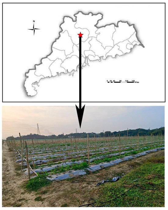
Figure 1.
Location of the experimental area in Guangdong.
The locations marked with stars indicate the approximate positions of our experimental sites. Through the management of farmers, the deviation of each row size in this chili field was small. The environment of the chili field is shown in Figure 2. The ridge height is 0.3 m, with a relatively narrow distance between the ridges. The distance between two rows of ridges is 0.75 m, and the width of a single ridge is 0.5 m.
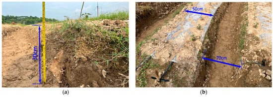
Figure 2.
(a) Ridge height in the experimental chili field; (b) The distance between the ridges and the width of the ridges in the experimental chili field.
According to the “Technical Regulations for Land Use Investigation”, chili fields are divided into flat land (≤2°, 2°~6°), gentle slope (6~15°, 15~25°), and steep land (>25°) according to the ground slope [33]. The ground slope between each ridge in the experimental chili field is 5°~15°, which belongs to the gentle slope. Through the maintenance and management of the field ridges and the ground between the ridges by chili growers, combined with agronomic practices, the above data will not exhibit significant deviation, effectively ensuring the accuracy and stability of the navigation system.
2.2. Multi-Sensor Data Fusion Positioning
2.2.1. Positioning Overall Scheme
Due to the relatively uneven terrain of chili fields, positioning drift is easily induced. To address this issue, this study proposes a positioning method based on multi-sensor fusion. In order to overcome the limitations of individual sensors and leverage the complementary advantages of different sensor data, the solution integrates LiDAR, the inertial measurement unit (IMU), and the global navigation satellite system (GNSS) for accurate positioning. Specifically, the RPLIDAR S2 LiDAR, WHEELTEC N200 IMU, and WHEELTEC DETA100 GNSS were selected. A series of data fusion processes were performed using the extended Kalman filter (EKF) algorithm running within the ROS unmanned system framework. The detailed node diagram is shown in Figure 3 below:
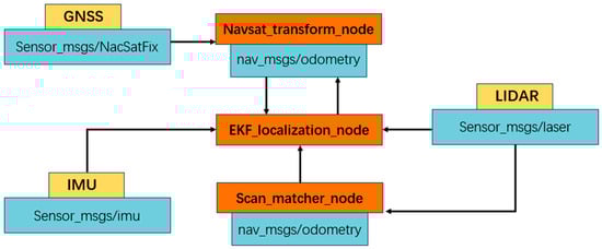
Figure 3.
Data fusion node diagram.
In the process of multi-sensor fusion, LiDAR primarily captures the structural characteristics of the external environment and accurately aligns it with the real map. The IMU provides orientation data along with continuous information about the robot’s speed and inclination angle, while the GNSS mainly assists in providing macro-level positional information. The data from these three sensors are fused using the extended Kalman filter (EKF) in combination with the adaptive Monte Carlo localization (AMCL) algorithm. This integration effectively leverages the high precision of LiDAR, the global positioning capabilities of the GNSS, and the short-term stability of the IMU. As a result, more accurate and reliable positioning results can be obtained. Accurate pose estimation and updates can not only improve the accuracy of positioning, but also maintain the continuity and accuracy of positioning through IMU and LiDAR information when GPS signals are weak or lost [34].
2.2.2. Data Fusion Analysis
Inaccurate positioning is a primary challenge that hinders reaching the target points in chili field navigation. To address this issue, this approach employs the extended Kalman filter (EKF) to perform data fusion of multiple sensors, including LiDAR, the GNSS global positioning system, and the IMU inertial navigation unit. This fusion enables the real-time determination of the vehicle’s precise position and orientation.
The extended Kalman filter (EKF) is an improved version of the Kalman filter (KF), which linearizes the nonlinear function through a Taylor series expansion, retaining only the first-order terms and neglecting higher-order terms. The Kalman filter algorithm is then applied to approximate both the system state and variance estimates. In the fusion of IMU and GNSS data, the IMU motion model and the GNSS measurement model typically exhibit nonlinearity. This is shown in Table 1 below.

Table 1.
Comparison of various filters.
The extended Kalman filter is a nonlinear expansion model of the standard Kalman filter.
The nonlinear system model can be expressed as follows:
Process noise:
Observed noise:
Equations (1)–(4) represent the state-space model of the system by introducing nonlinear state transition and observation models, where the state variables are presented in vector form. Due to the nonlinear nature of these models, the standard Kalman filter cannot be applied directly. Therefore, the EKF uses Taylor series expansion to linearize the nonlinear model and applies a Jacobian matrix to approximate these nonlinear relationships, thus treating it locally as a linear model.
In the prediction step, the EKF predicts the next state variable and its corresponding covariance using a nonlinear state transition model, as shown in Equations (5)–(7):
In the above formula,
is a linearized observation matrix, and
is the Jacobian matrix of the state transition model.
In the update step, Equations (8)–(10) calculate the Kalman gain by linearizing the observation model, using the Kalman gain to update the state estimates and their covariances:
Through these predictions and updating steps, the EKF can effectively provide approximate optimal estimates of states in nonlinear dynamic systems. The specific flow chart is as follows (Figure 4):
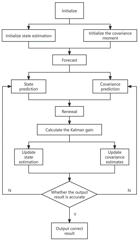
Figure 4.
Data fusion process diagram.
In this study, during multi-sensor fusion, each sensor operates independently and provides its own solution, which is then fused in a loosely coupled method to deliver comprehensive navigation information. Each sensor module functions independently, facilitating expansion and maintenance. This approach allows for the correction of errors introduced by sensor noise and environmental factors in the complex field environment. Additionally, system model uncertainty is addressed by adjusting the process noise covariance, enabling smooth state estimation, adjusting the filter response speed, optimizing the fusion effects of different sensors, and enhancing the filter’s stability and robustness. As a result, the fused data better meets the positioning requirements of chili field environments.
At the algorithm level, optimization measures are implemented in this study to address an issue where the fusion node cannot determine the position of the robot on the map. In the absence of a GNSS signal, incorrect information may be released. The master node is designed to subscribe to the filter odometry topic, published by the EKF node, to obtain the initial position. By creating data loops through mutual subscriptions, accuracy is improved and errors are minimized.
2.3. Optimize TEB Algorithm Construction and Analysis
The TEB (Timed Elastic Band) local path planning algorithm is an optimized path planning approach for autonomous robot navigation [35,36]. It achieves local optimization of the path by transforming the global path into an elastic band model, incorporating control points along the dynamic path.
The algorithm introduces some constraints such as fixed pose, obstacle, and kinematics. By applying mutual constraints on acceleration (a), velocity (v), arrival time (∆T), and distance from obstacles (s), the navigation system’s carrier avoids obstacles and reaches the target point at an optimal speed while satisfying kinematic requirements, thereby achieving efficient local path planning, as shown in Figure 5.
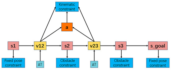
Figure 5.
Algorithm constraint.
The standalone use of the TEB algorithm for path optimization primarily employs nonlinear optimization techniques to generate and adjust paths, iteratively optimizing each feasible path across the entire space to find the optimal solution. However, this approach presents the following challenges: (1) The obstacle avoidance capability is limited, often leading to extreme collisions; (2) The high environmental complexity in chili fields reduces the accuracy of optimal path solutions. To address these issues, this study proposes cost function optimization for path smoothness to prevent abrupt motion changes, reduce the likelihood of extreme collisions, and enhance the safety of execution paths. Additionally, an uncertainty strategy optimization is applied to enable more flexible path adjustments, improving obstacle avoidance when encountering dynamic obstacles, sudden barriers, or other environmental changes. This study also integrates the A algorithm with the TEB algorithm, ensuring that the path aligns with the global objective while allowing real-time local path adjustments based on the global path during the planning process, thereby achieving a more rational and optimal path solution.
2.3.1. Cost Function Optimization for Path Smoothness
In the TEB algorithm, path smoothness is typically evaluated based on curvature. The original curvature cost function is derived by calculating the rate of directional change at each point along the path:
In the above formula,
θi is the direction angle of the i point on the path; s is the arc length on the path, representing the length of the path; and represents the rate of change of the direction angle with the arc length, that is, the curvature of the path.
For the narrow chili fields, the constraints of acceleration and angle change are introduced, and the dynamic weight parameters are designed:
In the above formula,
and are dynamically adjustable weight coefficients, and represents the acceleration of the change in angle.
When navigating along ridges, the path is narrow and uneven, and the obstacle density is high. Therefore, the weight of is increased to avoid sharp turns in the path as much as possible, so as to reduce the risk of collision. Conversely, when operating on relatively flat ground outside the chili field, where obstacle density is low, the weight of is adjusted to ensure the smoothness of the path and improve speed. By generating random target points, the trajectory data is obtained by running the improved planning algorithm in the virtual simulation environment. The trajectory diagram is plotted using the planar coordinates as the horizontal and vertical axes, as shown in Figure 6.
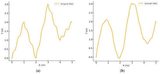
Figure 6.
(a) Original path; (b) Smooth path.
Obstacle-density detection is carried out using the method of grid division:
In the above formula,
Number of Obstacles in Cell indicates the number of obstacles detected in the current grid. Cell Area indicates the area of the grid.
The grid size is set to 0.1 m2, with a detection range of 100 × 100 grids. Due to the high density of obstacles between fields and ridges, the density threshold is set to 5. If the density exceeds the threshold, the weight of α is increased; if it is below the threshold, the weight of β is increased. The detection range moves dynamically with the navigation system carrier to enable real-time obstacle density detection.
2.3.2. Uncertainty Strategy Optimization
Chili fields contain numerous obstacles, such as people, animals, and other entities. By applying a conceptual collision method, a probabilistic obstacle avoidance strategy can assess the collision risk of different paths, and select the path with the lowest collision probability. Pcollision represents the collision probability.
In the above formula,
is the probability distribution of the robot at position x, and is the probability distribution of obstacles at position x.
By utilizing sensors such as LiDAR to acquire environmental information and representing obstacles and robots as probability distributions, collision risks can be more accurately assessed in dynamic and complex environments, allowing for the selection of safer paths. The optimization effect diagram is shown in Figure 7. As illustrated in Figure 7, compared to the original algorithm, the optimized algorithm demonstrates improved avoidance in areas with a high probability of obstacles.
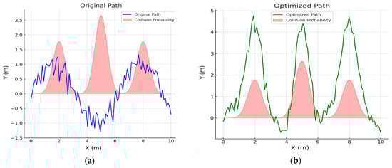
Figure 7.
(a) Original path; (b) Optimized path. Horizontal and vertical axes represent the simulated coordinate positions. The red area indicates the probability of collision between the planned path and the obstacle, and the higher the peak value, the greater the probability of collision.
2.3.3. Fusion Solution for Optimal Path
The fusion method of the A* algorithm and the TEB algorithm is employed to update the optimal initialization path for the TEB algorithm [37]. The formula and calculation process for initializing the path mainly involve two key functions: the heuristic function and the path cost function . Together, these two functions are used to compute the comprehensive evaluation function of node n:
In the above formula,
represents the actual path cost from the start node to the current node , and
is a heuristic function that estimates the cost from node to the target node. Setting this function requires: (1) not overestimating the cost from the node to the target node; (2) that for each node and its successor node , the following condition must be satisfied:
where is the actual cost from n to .
The actual fusion flow chart is shown in Figure 8.
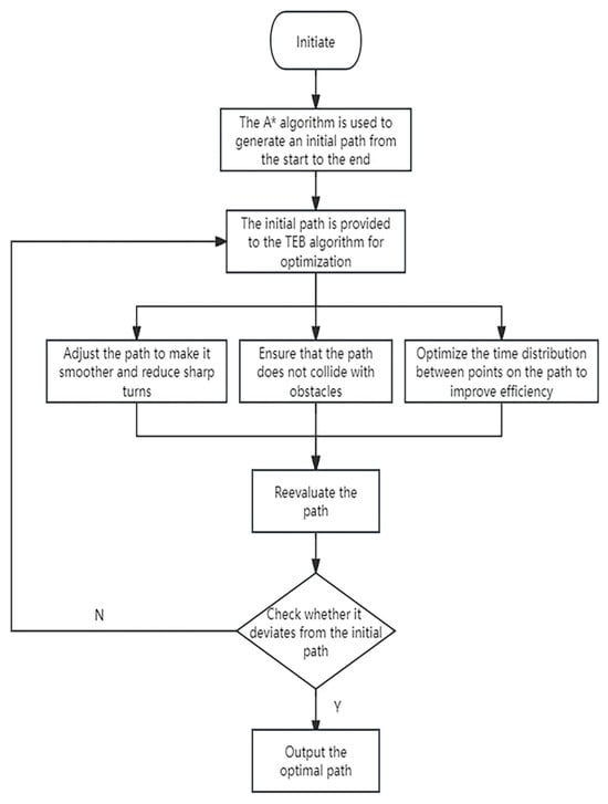
Figure 8.
Algorithm fusion process.
2.4. Experimental Design
In this section, we calibrate and validate the designed navigation system. Experimental tests are conducted to assess the positioning deviation of the positioning module within the navigation system, and to evaluate the effectiveness of the optimal path planning method.
The primary test vehicle in this study is the Pepperland Navigation Robot, shown in Figure 9. The navigation system was deployed on a Republic of Gamers laptop (G634, ASUS, Maricopa County, AZ, USA) equipped with an RTX 4080 discrete graphics card. The robot is equipped with an RPLIDAR S2 LiDAR (Pudong New District, Shanghai, China) featuring a scanning frequency of 10 Hz, a sampling frequency of 32k, and a scanning radius of up to 30 m. Additionally, it includes a WHEELTEC N200 nine-axis IMU inertial navigation module and a WHEELTEC DETA100 GNSS module. To ensure stable operation on steep terrains, the robot is also equipped with a custom-built tracked undercarriage.
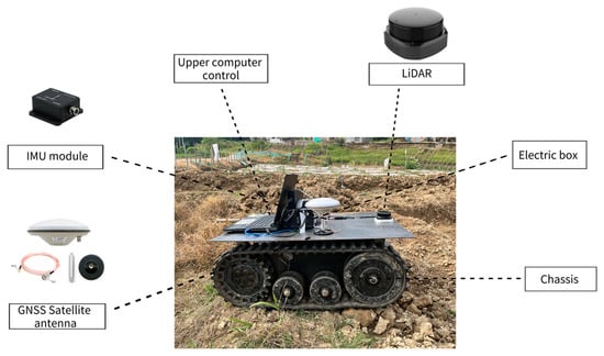
Figure 9.
Crawl-based chili field autonomous navigation vehicle.
All programs in the navigation system are implemented within the ROS framework, and the overall navigation process is illustrated in Figure 10.
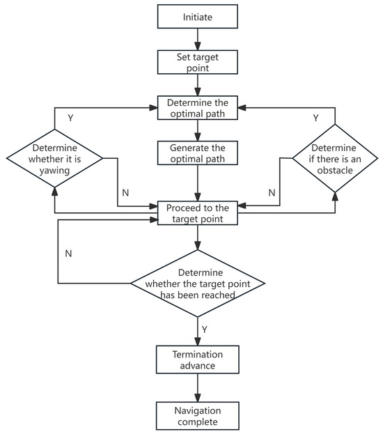
Figure 10.
Overall navigation system process.
Experimental Design of Chili Fields Navigation
In a chili field environment with a consistent slope, four different schemes were tested for positioning and navigation effectiveness: Scheme 1: Standard TEB algorithm + LiDAR; Scheme 2: Standard TEB algorithm + LiDAR +IMU+GNSS; Scheme 3: Optimize TEB algorithm + LiDAR; Scheme 4: Optimize TEB algorithm + LiDAR +IMU+GNSS in a chili field environment with the same slope.
The test area was established between the ridges of a typical chili field, as shown in Figure 11.
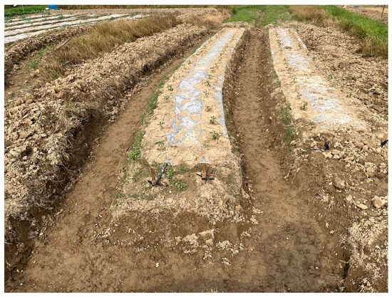
Figure 11.
Chili field scene for experiment.
In this experiment, the same starting point and target point were set, with a maximum speed of 0.5 m/s and a total distance of 10 m for each group. Each group was tested 10 times, with the number of collisions, the path length, the time consumption, and the target position offset recorded and calculated. The entire experimental procedure is shown in Figure 12:
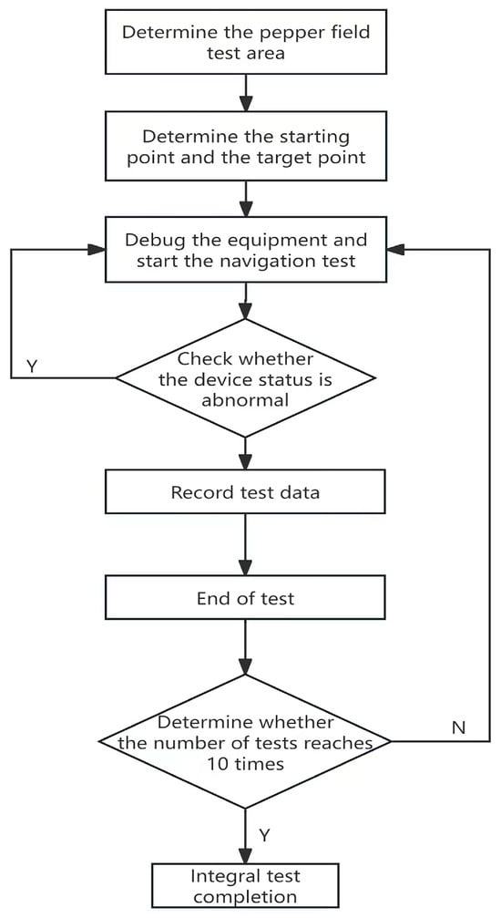
Figure 12.
Chili field navigation experiment process diagram.
The number of collisions is defined as the count of noticeable contacts between the robot and obstacles, such as ridges, throughout the entire navigation process. Path length is defined as the length of the navigation planned path between the start and the target points. Time consumption is defined as the average time taken by the robot to reach the target point from the starting point. The target position offset is defined as the distance between the robot’s actual position and the target point.
3. Results
The experiment was conducted in the test chili field under sunny conditions. A total of 10 groups of data for each scheme were collected, and the average value of the test results after collation and analysis is shown in Table 2.
Table 2.
The total number of collisions and the average value of each dataset.
The test results are presented in Table 2. It is observed that Scheme 1 has a relatively high collision frequency, reaching 8 instances. Multiple collisions occur during testing, with most collision points located at path inflection points. The average path length is 11.37 m, the average time consumption is 30.27 s, and the average target position offset is 8.35 cm. With the integration of the IMU inertial navigation system and the GNSS system, the number of collisions in Scheme 2 is reduced to 4 and the average target position offset decreases to 4.44 cm. Using the improved TEB algorithm, the collision frequency in Scheme 3 and Scheme 4 is further reduced to 6 and 1, respectively, showing a decreasing trend in collision frequency. Notably, Scheme 4 significantly reduces the probability of collisions with chili ridges. The average path length is reduced to 10.93 m and 10.79 m, the average time is shortened to 28.13 s and 27.72 s, and the average target position offset improves to 8.16 cm and 4.04 cm, respectively.
Comparing the data, the navigation system based on multi-sensor data fusion and the optimized TEB algorithm reduces the average planned path length by 0.58 m, shortens the average time from the starting point to the target by 2.55 s, and decreases the average target position offset by 4.3 cm. As shown in Figure 13, Scheme 4 exhibits less data variation compared to the previous three schemes, indicating an improvement in overall navigation stability.
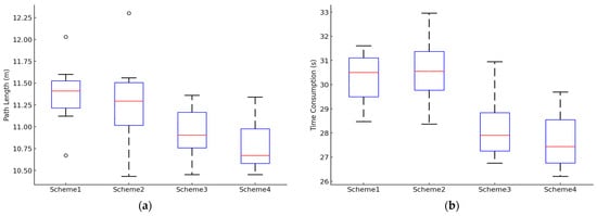
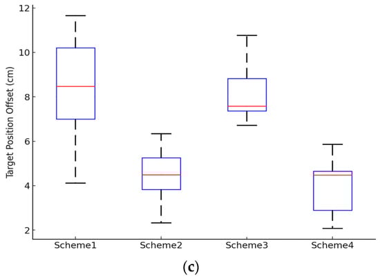
Figure 13.
(a) The value of path length in 10 experiments. (b) The value of time consumption in 10 experiments. (c) The value of the target position offset in 10 experiments.
In this study, SPSS v16.0 was used to perform independent sample t-tests on the experimental data. When examining the effect of multi-sensor data fusion, the p-values for time consumption and planned path length were 0.985 and 0.372, respectively, both greater than 0.05. This indicates that the choice between using LiDAR alone or LiDAR + IMU + GNSS has no significant impact on time consumption or planned path length. However, the p-value for target position offset was 4.3 × 10⁻⁹, less than 0.05, indicating a highly significant effect of multi-sensor data fusion on target position offset. Specifically, the use of LiDAR + IMU + GNSS significantly reduces target position offset compared to using LiDAR alone. When assessing the effect of the TEB algorithm, the p-value for target position offset was 0.720, greater than 0.05, suggesting that there is no significant difference in target position offset between the standard TEB algorithm and the optimized TEB algorithm. In contrast, the p-values for time consumption and planned path length were 4.4 × 10⁻⁴ and 1.2 × 10⁻⁷, respectively, both less than 0.05. This indicates that the choice between the standard TEB algorithm and the optimized TEB algorithm has a highly significant effect on time consumption and planned path length, with the optimized TEB algorithm performing better in both aspects.
4. Discussion
In this study, a navigation system for chili fields based on multi-sensor data fusion and an optimized TEB algorithm is proposed. The system utilizes the EKF to integrate data from LiDAR, the IMU, and the GNSS, and combines it with the optimized TEB algorithm using an A* algorithm. This is used to achieve accurate autonomous navigation in chili fields. The combined INS/GNSS navigation method based on a recurrent neural network (RNN) proposed by Dai et al. [21] may be limited by the training dataset in complex environments. When environmental conditions change, the model needs to be retrained. Zhong et al. used an integrated GPS/INS approach [20], which does not easily cope with the problem of slippage in chili fields. The scheme proposed by Abdelaziz et al. and Yu et al. is susceptible to ambient light [22,23]. The multi-sensor and optimized TEB algorithm-based navigation system proposed in this study can adapt to environmental changes in real time and can function effectively in varying slopes and slippery conditions typical of chili fields. Moreover, the system is minimally affected by lighting and is capable of operating continuously throughout the day, thereby enhancing operational efficiency in chili field applications. Dai et al.‘s study of local path planning algorithms for optimizing the TEB algorithm [32] was able to reduce the amount of smoothing of the speed control due to speed jumps, but it was still not effective enough to achieve safer path planning in narrow chili fields in order to reduce the number of collisions. Zhang et al. applied the artificial potential field method and dynamic window approach, respectively [38]. However, these methods are designed for path planning in relatively stable environments, and they have difficulty meeting the application requirements in the complex environment of chili pepper fields. The modified TEB algorithm proposed in this study, by introducing the constraints of acceleration and corner change and designing the dynamic weight parameters to make the modified TEB algorithm suitable for path planning in the narrow chili field environment, reduces the risk of collision, and is able to achieve more accurate autonomous navigation in the chili field to satisfy the needs of autonomous chili picking.
This study does have some limitations. The multi-sensor and optimized TEB algorithm-based chili field navigation system focuses on autonomous navigation in chili fields that are generally narrow in southern China, and its navigation methods may not be universally applicable to field navigation environments for all crops. In practical applications, the high computational volume of multi-sensor fusion and optimization algorithms can lead to insufficient arithmetic power of the master control system. Additionally, due to the narrow and complex environment, extreme collisions are still difficult to avoid completely. Future research should focus on enhancing the system’s applicability across a wider range of environments, addressing computational power limitations, and further reducing collision occurrences to improve versatility and effectiveness.
5. Conclusions
In this study, a multi-sensor- and optimized TEB algorithm-based navigation system for autonomous localization and navigation in chili fields is proposed. The system utilizes an extended Kalman filter to fuse data from LiDAR, the IMU, and the GNSS, optimizing the TEB algorithm for improved navigation performance. Experimental data collected in a real chili field environment demonstrate the effectiveness of the multi-sensor and optimized TEB algorithm-based navigation system. The results indicate that the system reduces the average value of the planned path length by 0.58 m, decreases the average time from the starting point to the target by 2.55 s, and reduces the average target position offset by 4.3 cm. Notably, the system significantly reduced collision frequency, with only one collision over ten experiments. The design of a multi-sensor- and optimized TEB algorithm-based navigation system for chili fields facilitates the subsequent development of chili picking fields and smart agriculture.
Author Contributions
Conceptualization, W.H., H.G. and Q.G.; methodology, W.H., H.G. and Q.G.; validation, W.H., R.X. and Q.G.; formal analysis, W.H., R.X. and Q.G.; investigation, W.H., Z.Z., R.X. and Y.G.; resources, W.H. and Y.G.; data curation, W.H., Q.G., Z.Z., H.G., X.F. and Y.G.; writing—original draft preparation, W.H., K.L. and Q.G.; writing—review and editing, Y.Z., X.F. and H.G.; visualization, W.H., K.L. and Q.G.; supervision, Y.Z.; project administration, Y.Z. and Y.G.; funding acquisition, Y.Z. and Y.G. All authors have read and agreed to the published version of the manuscript.
Funding
This research was funded by the Laboratory of Lingnan Modern Agriculture, grant number NT2021009, and the 111 Center, grant number D18019.
Data Availability Statement
Data is contained within the article.
Conflicts of Interest
The authors declare no conflicts of interest.
References
- Zou, X.; Ma, Y.; Dai, X.; Li, X.; Yang, S. Spread and Industry Development of Pepper in China. J. Hortic. 2020, 47, 1715–1726. [Google Scholar] [CrossRef]
- Lin, Q.; Xin, Z.; Kong, L.; Wang, X.; Yang, X.; He, W. Development status of China's chili pepper industry and breeding countermeasures. J. China Agric. Univ. 2023, 28, 82–95. [Google Scholar]
- Zhang, Z.; Zeng, L.; Zhang, W.; Ren, H.; Liu, L.; Zhang, Z.; Zou, X.; Qin, D.; Ou, L. Process Adaptability Appraisal of Fermented Chopped Chili Pepper Made from Fresh Chili Peppers of Different Varieties. Agronomy 2024, 14, 1833. [Google Scholar] [CrossRef]
- Lillywhite, J.; Tso, S. Consumers within the Spicy Pepper Supply Chain. Agronomy 2021, 11, 2040. [Google Scholar] [CrossRef]
- Zou, Z.; Zou, X. Geographical and Ecological Differences in Pepper Cultivation and Consumption in China. Front. Nutr. 2021, 8, 718517. [Google Scholar] [CrossRef]
- Qiao, L.; Zhao, B.; Zong, Y.; Kou, C.; Dong, Y. Development status, trend and countermeasures of chili industry in China. Chin. Veg. 2023, 11, 9–15. [Google Scholar]
- Wang, L.; Ma, Y.; Zhang, B. Market demand and breeding trend of chili pepper varieties in China. Chin. Veg. 2019, 8, 1–4. [Google Scholar] [CrossRef]
- Wang, D.; Huo, X.; Zong, Y.; Jia, H. The Current Status and Suggestions for High-Quality Development of the ”Jize Chili” Industry. North. Horticult. 2024, 20, 131–136. [Google Scholar]
- Deng, C.; Zhong, Q.; Shao, D.; Ren, Y.; Li, Q.; Wen, J.; Li, J. Potential Suitable Habitats of Chili Pepper in China under Climate Change. Plants 2024, 13, 1027. [Google Scholar] [CrossRef]
- Wang, L.; Zhang, B.; Zhang, Z.; Cao, Y.; Yu, H.; Feng, X. Research progress, industrial status and outlook of chili pepper breeding in China during the 13th Five-Year Plan. Chin. Veg. 2021, 2, 21–29. [Google Scholar] [CrossRef]
- Fu, J.; Ji, C.; Liu, H.; Wang, W.; Zhang, G.; Gao, Y.; Zhou, Y.; Abdeen, M. Research Progress and Prospect of Mechanized Harvesting Technology in the First Season of Ratoon Rice. Agriculture 2022, 12, 620. [Google Scholar] [CrossRef]
- Zhang, M.; Ji, Y.; Li, S.; Cao, R.; Xu, H.; Zhang, Z. Progress of agricultural machinery navigation technology. J. Agric. Mach. 2020, 51, 1–18. [Google Scholar]
- Xie, B.; Jin, Y.; Faheem, M.; Gao, W.; Liu, J.; Jiang, H.; Cai, L.; Li, Y. Research progress of autonomous navigation technology for multi-agricultural scenes. Comput. Electron. Agric. 2023, 211, 107963. [Google Scholar] [CrossRef]
- Botta, A.; Cavallone, P.; Baglieri, L.; Colucci, G.; Tagliavini, L.; Quaglia, G. A Review of Robots, Perception, and Tasks in Precision Agriculture. Appl. Mech. 2022, 3, 830–854. [Google Scholar] [CrossRef]
- Tan, C.; Li, Y.; Wang, D.; Mao, W.; Yang, F. Research progress of automatic navigation technology of agricultural machinery. Agric. Mech. Res. 2020, 42, 7–14+32. [Google Scholar] [CrossRef]
- Cui, B.; Zhang, J.; Wei, X.; Cui, X.; Sun, Z.; Zhao, Y.; Liu, Y. Improved Information Fusion for Agricultural Machinery Navigation Based on Context-Constrained Kalman Filter and Dual-Antenna RTK. Actuators 2024, 13, 160. [Google Scholar] [CrossRef]
- Chen, T.; Xu, L.; Ahn, H.; Lu, E.; Liu, Y.; Xu, R. Evaluation of headland turning types of adjacent parallel paths for combine harvesters. Biosyst. Eng. 2023, 233, 93–113. [Google Scholar] [CrossRef]
- Wang, W.; Xing, C.; Feng, W. Development status and trend of autonomous navigation technology. J. Aviat. 2021, 42, 18–36. [Google Scholar]
- Gao, Q.; Lu, K.; Ji, Y.; Liu, J.; Xu, L.; Wei, G. A review of multi-sensor fusion SLAM research. Mod. Radar 2024, 46, 29–39. [Google Scholar]
- Zhong, Y.; Xue, M.; Yuan, H. Design of combined GNSS/INS navigation system for intelligent agricultural machines. J. Agric. Eng. 2021, 37, 40–46. [Google Scholar]
- Dai, H.; Bian, H.; Wang, R.; Ma, H. An INS/GNSS integrated navigation in GNSS denied environment using recurrent neural network. Def. Technol. 2020, 16, 334–340. [Google Scholar] [CrossRef]
- Abdelaziz, N.; El-Rabbany, A. Deep Learning-Aided Inertial/Visual/LiDAR Integration for GNSS-Challenging Environments. Sensors 2023, 23, 6019. [Google Scholar] [CrossRef] [PubMed]
- Yu, J.; Lu, W.; Zeng, M.; Zhao, S. Multi-sensor fusion low-cost automatic navigation method for agricultural machines. China Test 2021, 47, 106–113+119. [Google Scholar]
- Yu, J.; Chen, Y.; Feng, C.; Su, Y.; Guo, J. A review on local path planning for intelligent construction robots. Comput. Eng. Appl. 2024, 60, 16–29. [Google Scholar]
- Zheng, K.; Han, B.; Wang, X. Ackerman robot motion planning system based on improved TEB algorithm. Sci. Technol. Eng. 2020, 20, 3997–4003. [Google Scholar]
- Chen, Y.; Shen, J.; Li, S. Research on dynamic obstacle avoidance strategy for multiple robots with improved TEB algorithm. Electro-Opt. Control. 2022, 29, 107–112. [Google Scholar]
- Chen, J.; Guo, C.; Liu, Y. A mobile robot path optimization method based on temporal elastic band. Sci. Technol. Eng. 2021, 21, 11212–11219. [Google Scholar]
- Wu, T.; Xie, Z.; Chen, K. Improved D*lite and time-elastic band method for mobile robot path planning. J. Sens. Technol. 2022, 35, 486–494. [Google Scholar]
- Chen, H.; Dou, P.; Cheng, C.; Wang, Z. Multi-objective point path planning in wind turbine waters based on Bi-RRT and TEB algorithms. Mar. Eng. 2024, 53, 130–136. [Google Scholar]
- Yin, X.; Dong, W.; Wang, X.; Yu, Y.; Yao, D. Route planning of mobile robot based on improved RRT star and TEB algorithm. Sci. Rep. 2024, 14, 8942. [Google Scholar] [CrossRef]
- Dai, W.; Zhang, L.; Wu, J.; Ma, X. Research on local path planning algorithm with improved TEB algorithm. Comput. Eng. Appl. 2022, 58, 283–288. [Google Scholar]
- Yang, J.; Qin, X.; Lei, J.; Lu, L.; Zhang, J.; Wang, Z. Design and Experiment of a Crawler-Type Harvester for Red Cluster Peppers in Hilly and Mountainous Regions. Agriculture 2024, 14, 1742. [Google Scholar] [CrossRef]
- Wang, K.; Zhang, J.; Xu, Z.; Xu, Y. Interpretation of Land Use Planning Technical Regulations Based on Integration and Oriented to Transformation—”Urban Land Use Classification and Planning Land Use Standards (GB50137-2011)”. Urban Plan. 2012, 36, 42–48+92. [Google Scholar]
- Deng, P.; Luo, J. Robot Multi-sensor Fusion positioning Method in Complex Environment. Chin. J. Electron. Meas. Instrum. 2023, 37, 48–57. [Google Scholar]
- Zhang, S.; Zhang, Q.; Wang, G.; Wu, L.; Cai, Z.; Li, Y.; Lin, Z. A Combined Navigation Path Planning Method Based on Improved A* and Optimized TEB. Laser Mag. 2024, 45, 39–46. [Google Scholar]
- Luan, T.; Wang, H.; You, B.; Sun, M. A Pose-Assisted Point TEB Navigation Method for Autonomous Vehicles in Narrow Spaces. J. Instrum. Sci. Technol. 2023, 44, 121–128. [Google Scholar]
- Lv, Z.; Ni, L.; Peng, H.; Zhou, K.; Zhao, D.; Qu, G.; Yuan, W.; Gao, Y.; Zhang, Q. Research on Global Off-Road Path Planning Based on Improved A* Algorithm. ISPRS Int. J. Geo-Inf. 2024, 13, 362. [Google Scholar] [CrossRef]
- Zhang, Y.; Song, J.; Zhang, Q. Local Path Planning of Outdoor Cleaning Robot Based on an Improved DWA. Robot 2020, 42, 617–625. [Google Scholar] [CrossRef]
Disclaimer/Publisher’s Note: The statements, opinions and data contained in all publications are solely those of the individual author(s) and contributor(s) and not of MDPI and/or the editor(s). MDPI and/or the editor(s) disclaim responsibility for any injury to people or property resulting from any ideas, methods, instructions or products referred to in the content. |
© 2024 by the authors. Licensee MDPI, Basel, Switzerland. This article is an open access article distributed under the terms and conditions of the Creative Commons Attribution (CC BY) license (https://creativecommons.org/licenses/by/4.0/).