TomatoPoseNet: An Efficient Keypoint-Based 6D Pose Estimation Model for Non-Destructive Tomato Harvesting

Abstract

The non-destructive harvesting of fresh tomatoes with agricultural robots requires the robotic arm to approach the fruit with the correct posture to ensure successful harvesting. However, this process faces significant challenges due to the small size of fruit pedicels, cluttered environments, and varied poses of the tomatoes and pedicels. Accurately identifying, localizing, and estimating the 6D spatial pose of the cutting points is critical for efficient and non-destructive harvesting. To address these challenges, we propose a keypoint-based pose estimation model, TomatoPoseNet, tailored to meet the agronomic requirements of tomato harvesting. The model integrates an efficient fusion block (EFBlock) based on the CSPLayer, referred to as the CSEFLayer, as the backbone network, designed to fuse multiscale features while maintaining efficient computational resource usage. Next, a parallel deep fusion network (PDFN) is utilized as the neck network to integrate features from multiple parallel branches. Furthermore, simple coordinate classification (SimCC) is employed as the head network for keypoint detection, and a StripPooling block is introduced to enhance the model’s ability to capture features of different scales and shapes by applying strip pooling in horizontal and vertical directions. Finally, a geometric model is constructed based on the information about the predicted 3D keypoints to estimate the 6D pose of the cutting points. The results show the following: (1) The average precision for keypoint detection (PCK@0.05) reached 82.51%, surpassing those of ViTPose, HRNet, Lite-HRNet, Hourglass, and RTMPose by 3.78%, 9.46%, 11%, 9.14%, and 10.07%, respectively. (2) The mean absolute errors (MAEs) of the yaw and pitch angles for 6D pose estimation of the cutting points were 2.98° and 3.54°, respectively, with maximum errors within 6.5°, meeting the requirements for harvesting. The experimental results demonstrate that the proposed method can accurately locate the 6D pose of cutting points in an unstructured tomato harvesting environment, enabling non-destructive harvesting.

1. Introduction

Developing efficient, non-destructive automated harvesting systems has been a primary focus of agricultural automation and robotics research, particularly for delicate crops such as tomatoes, where precise harvesting is essential to prevent damage. Vision systems play a crucial role in autonomous harvesting by enabling robots to accurately identify harvesting points and estimate the 6D pose of tomatoes based on their specific characteristics. With this information, the robotic arm approaches the fruit with the correct posture to ensure successful harvesting [1,2]. However, accurately identifying the stem position and estimating the fruit’s pose remain significant challenges in non-destructive harvesting. Existing methods often struggle to reliably locate stems in complex environments, especially when the stems are thin or partially obscured by surrounding fruits or leaves. As a result, the effectiveness of autonomous harvesting depends heavily on vision algorithms that are capable of accurate crop recognition and pose estimation [3].

In recent years, the application of deep learning technology has significantly advanced the development of automated harvesting robots, with its advantages being particularly evident in fruit target detection. For instance, Huang et al. [4] designed a lightweight network called GCS-YOLOv4 for multi-stage fruit detection with improved detection speed and accuracy. Wang et al. [5] introduced an improved lightweight SM-YOLOv5 algorithm for tomato detection, which added a small-object detection layer, achieving model simplification and enhanced accuracy in detecting small fruit targets. Yang et al. [6] utilized the YOLOv8 model for tomato detection, reducing computational complexity through DSConv, and improving accuracy by incorporating dual-path attention gates and the FEM module. These studies demonstrate that deep learning-based object detection technology can successfully perform detection tasks in complex agricultural environments. However, most of this research has focused on providing positional information for fruit grasping while neglecting fruit pose information. Accurate pose information is crucial for ensuring that harvesting robots avoid collisions with obstacles such as stems and the surrounding environment during picking, thereby preventing damage to the fruit.

Two primary methods are commonly used for fruit harvesting: plucking and cutting. The plucking method involves twisting, bending, or pulling the fruit to separate it from the branch, making it relatively simple. However, directly grasping the fruit body may cause damage to the skin, potentially affecting the quality of the fruit. In contrast, the cutting method requires additional detection of the stem’s cutting point, although, this method, which separates the fruit by directly severing the stem, can effectively reduce dependency on varying fruit shapes if the cutting point is accurately detected [7]. In recent years, stem detection has seen increasing application in cutting-based harvesting robots. For instance, Rong et al. [8] used the Yolov4-Tiny model to detect cherry tomato clusters and then employed the YOLACT++ model to segment the stems from the clusters; they also proposed a method for locating the cutting point and estimating the stem pose for cherry tomatoes. Similarly, Zhong et al. [9] used YOLACT to segment lychee clusters and stems and applied the least squares method to fit the stems and estimate the pose of the picking point. Although stem detection technology has made significant progress in real-world environments, its application in harvesting robots still faces numerous challenges. In most cases, stem detection methods consist of multiple stages, relying on geometric features, morphological factors, and line-fitting techniques to detect the fruit and its stem. These complex processes increase computational complexity and may introduce cumulative errors at each stage, ultimately affecting the detection accuracy.

To address these limitations, keypoint detection methods have gained attention in agriculture. Keypoint-based pose estimation allows for a more direct estimation of pose by detecting specific keypoints on the target object, eliminating the need for multi-stage processing. This method is particularly effective in handling occlusions and small-scale features, such as stems, within complex backgrounds. In recent years, keypoint-based pose estimation has emerged as a critical research area in deep learning, enabling pose estimation through a straightforward process of detecting connections between keypoints on an object. This approach has been widely applied in human skeleton and joint extraction but has seen limited use in agriculture [10]. Zhang et al. [11] proposed a 3D pose detection method for tomato clusters, referred to as the Tomato Pose Method (TPM); utilizing a cascaded object and keypoint detection network, they detected the bounding box and 11 keypoints of the tomato clusters. Jiang et al. [12] introduced the YOLOv8n-GP keypoint detection model to estimate the pose of grape stems, but it only predicted the 2D pose in images. Kim et al. [13] used the OpenPose keypoint detection model to estimate the 2D pose of tomatoes and combined it with depth maps to estimate the 3D pose; however, the accuracy of the 3D pose estimation was not evaluated. Zhang et al. [14] further developed the Tomato Pose Method (TPMv2) using deep neural networks to detect 2D and 3D keypoints of tomato clusters simultaneously; however, due to the lack of comparison with ground-truth geometric measurements of tomatoes in actual greenhouses, the accuracy of their pose estimation could not be confirmed. Ci et al. [15] proposed an innovative method to estimate the 3D pose of tomato peduncle nodes from RGB-D images, providing complete 3D pose information necessary for robotic manipulation. These approaches use keypoint information combined with point cloud data to estimate the 3D pose of fruits. When harvesting tomatoes, it is crucial to consider the 6D information of the cutting point in order to prevent collisions between the robot’s end-effector and the fruit.

Thus, this paper proposes a keypoint-detection-based approach that combines the advantages of 2D keypoint detection networks with point cloud processing techniques to estimate the full 6D pose of the tomato stem’s cutting point, enabling robotic harvesting operations. Specifically, the main contributions of this work are as follows:

• A TomatoPoseNet 2D keypoint detection model is proposed, which defines four keypoints and combines RGB-D images to estimate the 3D pose of these keypoints.
• A geometric model is developed to estimate the 6D pose of the tomato pedicel’s cutting point by integrating 3D keypoint pose information.
• The accuracy of the estimated 6D pose in real-world coordinates is evaluated in a greenhouse tomato cultivation environment, comparing it against manual measurements.

2. Materials and Methods

2.1. Data Acquisition

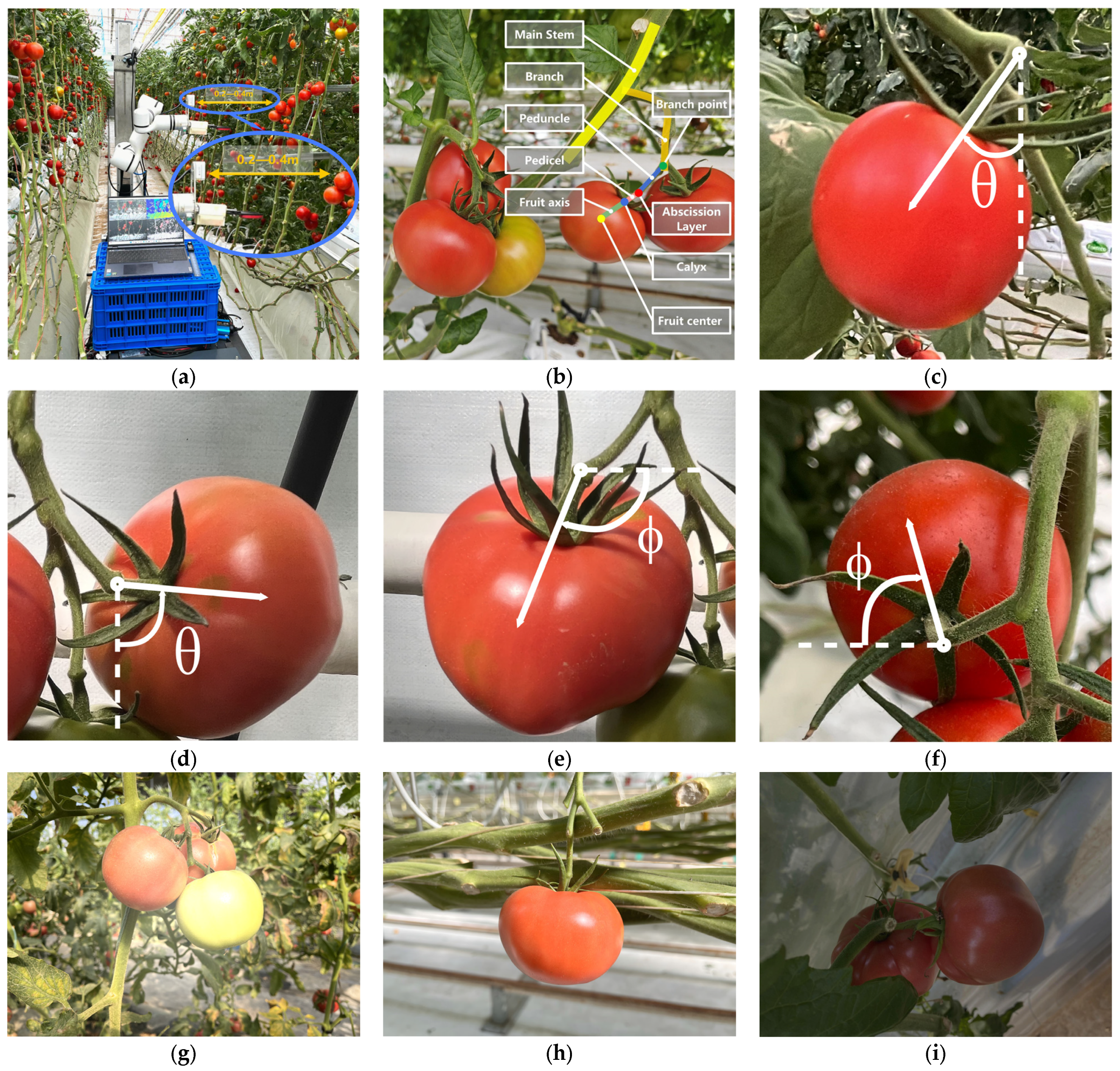
From October 2023 to May 2024, images were captured using an Intel RealSense D405 RGB-D camera at the Zhongguancun Smart Vegetable Factory in Beijing, China (40.176475 N, 117.018911 E). The greenhouse adhered to the standard Dutch planting and management model. The tomatoes cultivated were of the Hong Zhen Zhu variety, which grows in clusters containing one to four fruits. These tomatoes are large, grow closely together, and are often pressed against one another. Due to their weight, the primary and secondary stems exhibit varying degrees of deformation, resulting in various orientations and poses of the fruit clusters.

The D405 camera is specifically designed for close-range depth sensing, featuring a depth output resolution of 1280 × 720 pixels and an ideal depth measurement range of 70 mm to 500 mm; it employs global shutter exposure and binocular stereo vision technology, offering a wide field of view of 87° (horizontal) × 58° (vertical). In this study, the camera was mounted on the end-effector of a robotic arm, positioned at a distance of 200 to 400 mm from the tomatoes, as illustrated in Figure 1a. This setup ensured that the camera operated within its optimal measurement range, guaranteeing high depth measurement accuracy (±2% at 500 mm).

During the data acquisition process, images were captured under various growth stages and lighting conditions as the mobile platform moved to ensure the adaptability of the harvesting robot’s vision system in unstructured environments. In total, 1100 images were collected. Figure 1c–f display examples of tomato clusters in various poses. These samples ensure diversity in the dataset, representing different growth periods and lighting conditions.

2.2. Description of the Tomato Fruit–Stem System

The main stem of a tomato plant can support one or more fruit clusters [16] (Figure 1b). These clusters are connected to the plant’s main stem via branches, and each fruit is attached to the pedicel, which, in turn, connects to the branch of the fruit cluster. Once the tomato ripens, a weak abscission layer forms at the connection point between the pedicel and the peduncle, making it easier to detach during harvesting. According to agricultural standards, harvested tomatoes should retain the calyx and a small portion of the pedicel to aid in storage and prevent damage during transportation. Therefore, the optimal harvesting points are the abscission (where the pedicel meets the peduncle) and the section of the pedicel near the calyx.

In this study, the pose of the tomato fruit–stem system was defined using four keypoints: (1) branch point, (2) abscission, (3) calyx, and (4) fruit center [13]. These keypoints were determined by identifying the center of the relevant areas, as shown in Figure 2a. When the shape of the fruit is approximately circular, Keypoint 4 is located at the center of the circle, representing the fruit center. Keypoint 3 is the center of the connection between the calyx and the pedicel. Keypoint 2 is the center of the abscission, while Keypoint 1, defined in this study as the branch point, is located at the center of the connection between the branch and the peduncle. The adjacent keypoints are connected to represent the geometric relationships between them, which are critical for determining the pose of the tomato fruit–stem system. Keypoints 1–2, 2–3, and 3–4 are connected by the peduncle, pedicel, and fruit axis, respectively [13,16]. Figure 2 shows the structure of the tomato plant. Accurately estimating the position of these keypoints can provide comprehensive geometric information for tomato harvesting, thereby improving both efficiency and quality.

2.3. Data Annotation

In this study, we used Labelme to annotate keypoints and bounding boxes. Figure 2b depicts the keypoint dataset, comprising annotated keypoints and bounding boxes. We categorized the tomatoes into two groups based on maturity: mature and immature. Each bounding box contained four keypoints corresponding to the same category: (1) branch point, (2) abscission, (3) calyx, and (4) fruit center. We did not annotate keypoints that were severely occluded and, thus, invisible. The proportion of invisible keypoints was relatively low across the entire tomato dataset. We stored the locations of all bounding boxes and keypoints in corresponding JSON files.

To ensure randomness during dataset construction, we randomly divided all 1100 annotated images into training, validation, and test sets, following an 8:1:1 ratio. The distribution of images under different lighting conditions is shown in

Table 1. Dataset division under different lighting conditions (by number of images).

Set	Strong Light	Natural Light	Low Light	Total
Training	275	329	276	880
Validation	36	42	32	110
Testing	36	47	27	110

, while

Table 2. Number of keypoint labels by category (in units).

Set	Branch Point	Abscission	Calyx	Fruit Center	Total
Training	501	610	719	754	2584
Validation	80	78	87	89	334
Testing	95	100	126	130	451

presents the number of labeled keypoints for each category.

2.4. Framework for 6D Pose Estimation of the Cutting Point

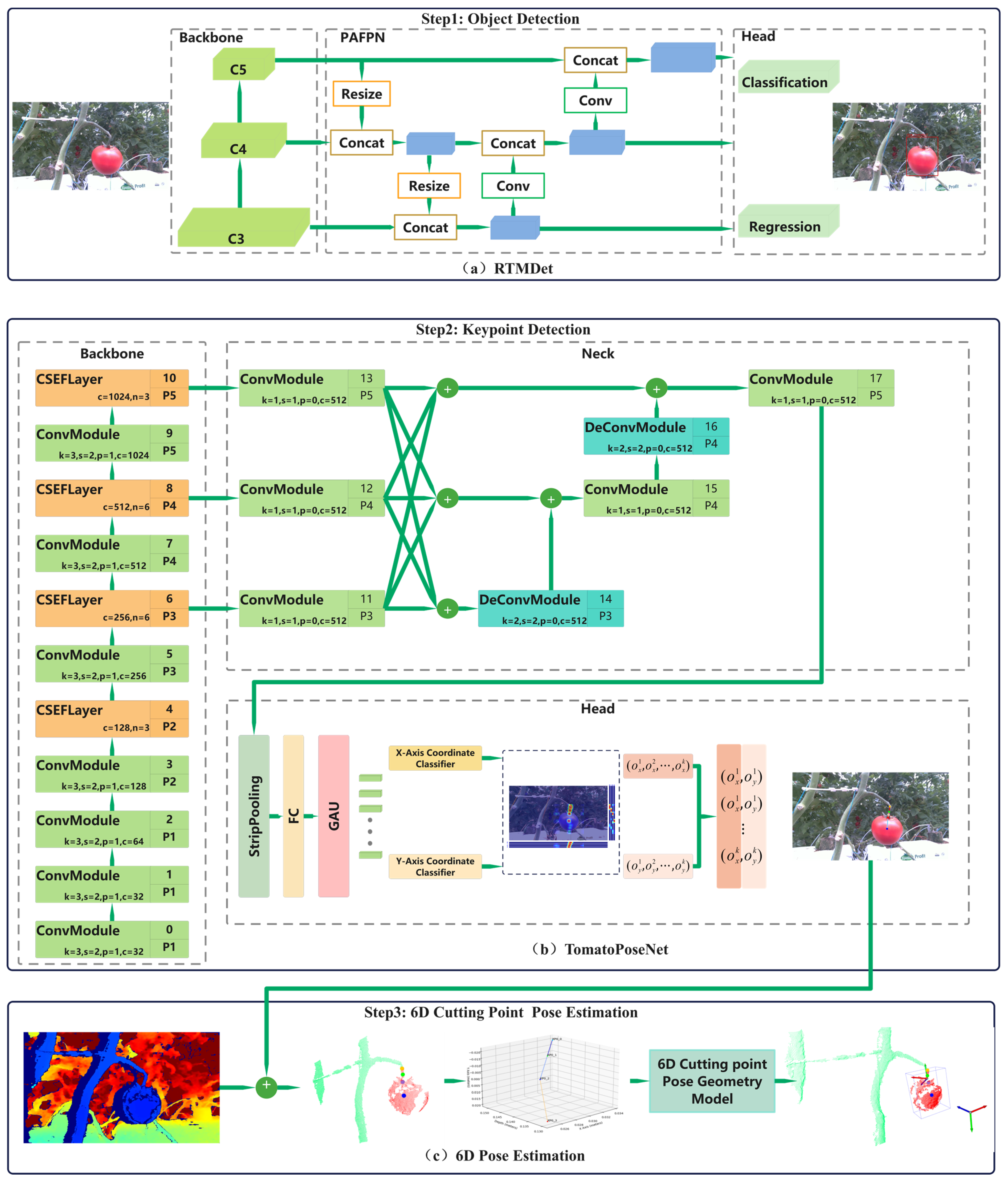
This paper proposes a framework for 6D pose estimation of the cutting point, as illustrated in Figure 3. The framework employs a top–down approach for keypoint detection, combined with 3D information for pose estimation, and consists of three main stages [1,3,4,5,6,7]: The first stage involves object detection. Real-time images captured by the RGB-D camera are processed through the object detection network to identify the region of interest (ROI) corresponding to the bounding box surrounding the target.

The second stage is keypoint detection. Together with object detection, this forms a complete top–down keypoint detection process, as illustrated in Figure 3b. In this stage, the detected ROI is cropped and passed to a specialized keypoint detection network, which infers the precise 2D coordinates of keypoints within the ROI, including the base of the pedicel (near the calyx) and the pedicel tip (near the abscission). The RGB image is aligned with the registered depth map to generate point cloud data. By matching the predicted 2D keypoint coordinates with the point cloud, we can obtain the corresponding 3D positions of these keypoints.

The third stage involves a 6D pose estimation of the cutting point, as illustrated in Figure 3c. Using the 3D coordinates of the two pedicel keypoints obtained from the previous stages, and based on agricultural requirements and the proportional length of the pedicel, the cutting point is determined to be located at a position half of the pedicel’s length from the calyx. The 6D pose of the cutting point, including its 3D position and orientation, is calculated using a geometric model with the pedicel’s direction vector as an input.

2.5. Object Detection Network

To balance inference speed and accuracy, RTMDet-m [17], the medium-scale version of the real-time object detection model (RTMDet), was selected as our candidate detector, as shown in Figure 3a. RTMDet is a high-precision, low-latency, one-stage object detection model that has demonstrated outstanding performance on the COCO 2017 dataset. The RTMDet-m model utilizes CSP blocks and large-kernel depth convolution layers in its backbone network, effectively expanding the receptive field. Multiple feature layers, including C3, C4, and C5, are extracted from the backbone and integrated into the CSP-PAFPN module, which shares the same architecture as the backbone network. The detection head uses shared convolutional weights and independent batch normalization (BN) layers to predict classification and regression results for the bounding boxes.

2.6. Keypoint Detection

This paper presents a top–down real-time keypoint estimation model, TomatoPoseNet, as shown in Figure 3b. The model first employs a pretrained object detector to obtain bounding boxes, followed by keypoint estimation within the detected objects. The backbone network of TomatoPoseNet is constructed using the CSEFLayer, demonstrating strong feature fusion capabilities. Multiscale features labeled as C3, C4, and C5 are extracted from the backbone and fused in the DFPM neck network, which shares a similar architecture with the backbone. The head network, an improved version of SimCC [18], is then used for keypoint detection.

2.6.1. Backbone

To enhance the feature fusion capability and computational efficiency of the network, CSEFLayer was chosen as the backbone, further integrating the efficient fusion block (EFBlock) into the CSPLayer [17]. The aim was to fuse multiscale features while efficiently using computational resources.

EFBlock is a highly efficient downsampling–upsampling module that preserves the richness of deep features while restoring spatial resolution; it uses depthwise separable residual blocks (DWResBlock), as shown in the top-right panel of Figure 4, for efficient feature extraction while reducing parameter counts. MaxPooling layers capture broader context information, and deconvolution layers are used to restore feature map details. EFBlock leverages residual connections with CSPLayer and uses 1 × 1 convolution for final feature fusion, ensuring consistency across feature channels.

To improve computational efficiency without sacrificing the representational power of convolutional neural networks (CNNs) [19], DWResBlock was introduced. This structure enhances traditional residual blocks by incorporating depthwise separable convolutions, decomposing standard convolutions into depthwise and pointwise convolutions, and reducing the computational cost and model complexity.

The computation process of DWResBlock can be formalized by the following expression:

$$\begin{array}{c}F(x)=Con{v}_{1\times 1}\left(DwConvBN\left(\left(Con{v}_{3\times 3}(x)\right)\right)\right.\\ H(x)=F(x)+Con{v}_{1\times 1}(x)\end{array}$$

(1)

where ${ \mathrm{Conv}}_{3\times 3}$ refers to a convolution layer with a 3 × 3 kernel, a stride of 1, and padding with the same edges; $\mathrm{Dwconv}$ indicates the depthwise convolution operation performed on the input feature map x; $BN$ stands for batch normalization; and $Con{v}_{1\times 1}$ represents a pointwise convolution layer. After residual block processing, the function $H_{1\times 1}$ denotes the output feature map.

2.6.2. Parallel Deep Fusion Network (PDFN) for Feature Integration

In traditional network architectures, high-resolution input images are typically downsampled and encoded into low-resolution feature representations, followed by upsampling for decoding back to high resolution. While this reduces the computational complexity, it also results in the loss of fine-grained details from the original image. For keypoint estimation tasks requiring precise spatial details, it is critical to retain sufficient spatial information to locate the keypoints accurately.

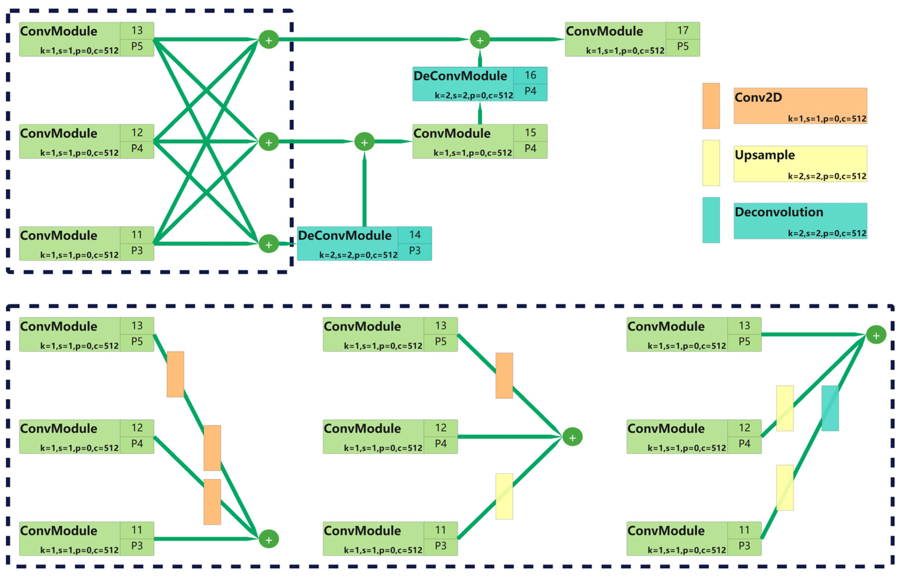
To address this, we designed a parallel deep fusion network (PDFN) (as shown in Figure 5) as the neck, which includes three primary feature layers. These layers (C3, C4, and C5) are processed using 1 × 1 convolutions to unify the channel dimensions, optimizing the information flow and ensuring consistency during feature fusion. The feature fusion module integrates information from different resolutions, inspired by HRNet [20]. The module sums high-resolution features with upsampled low-resolution features, and vice versa, to create more enriched feature maps. The upsampling operation uses nearest-neighbor interpolation and deconvolution, while downsampling is achieved with a stride of 2 and a 3 × 3 convolution kernel.

To ensure smooth transitions between high-resolution and low-resolution features, a multilevel fusion strategy inspired by DAPPM [21] was employed. This strategy incrementally upsamples feature maps, ensuring that features at different resolutions can effectively merge before final fusion.

The upsampling operation is achieved by using deconvolution to restore low-resolution feature maps to higher resolution. Additionally, convolution layers are used for further feature extraction, enhancing the network’s ability to capture detailed information. The upsampling and fusion processes effectively combine high- and low-resolution feature maps.

2.6.3. SimCC Head and StripPooling for Enhanced Feature Capture

The SimCC (simple coordinate classification) [18] head network is used for keypoint detection. This method converts the keypoint localization problem into independent classification tasks for the x and y coordinates. Compared to traditional heatmap regression methods, SimCC offers higher computational efficiency, accuracy, and stability, enabling pixel-level localization precision while simplifying the model structure.

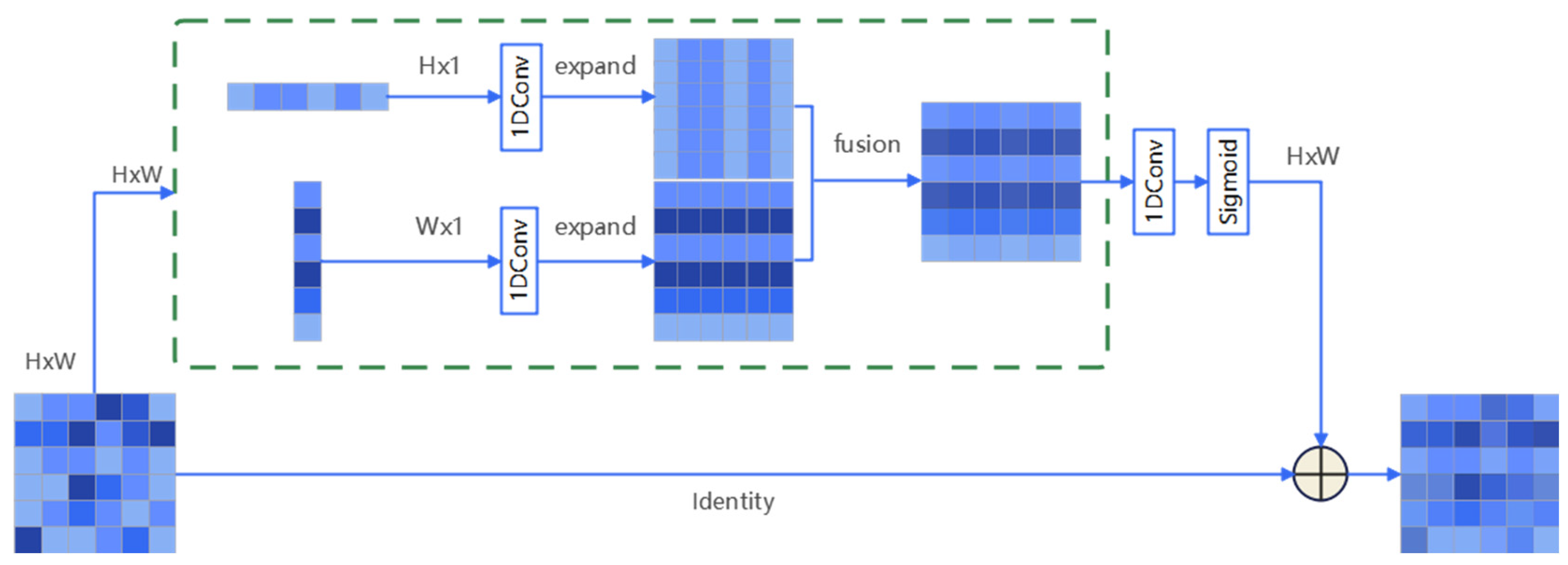
To enhance the model’s ability to capture long-range dependencies and global context, a StripPooling block [22] was introduced between the neck and the SimCC head. This block applies strip pooling in horizontal and vertical directions, improving the model’s perception of different scales and shapes.

The StripPooling processes in Figure 6 are represented by an H × W feature map, where H and W represent the height and width, respectively. The process applies two independent 1D convolution operations on the height and width dimensions to generate horizontal and vertical feature maps. These feature maps are then transformed into 2D feature planes, enabling integration with the original feature map. The fused feature maps are processed with a 1D convolution and sigmoid activation to produce an attention map multiplied by the original feature map to apply a dynamic attention mechanism. The final output is obtained by means of the element-wise addition of the attention-weighted feature map and the original feature map.

Integrating the StripPooling module significantly improved the model’s performance on various benchmark tests. Detailed experimental results are reported in subsequent sections.

2.7. Cutting Point Pose Estimation

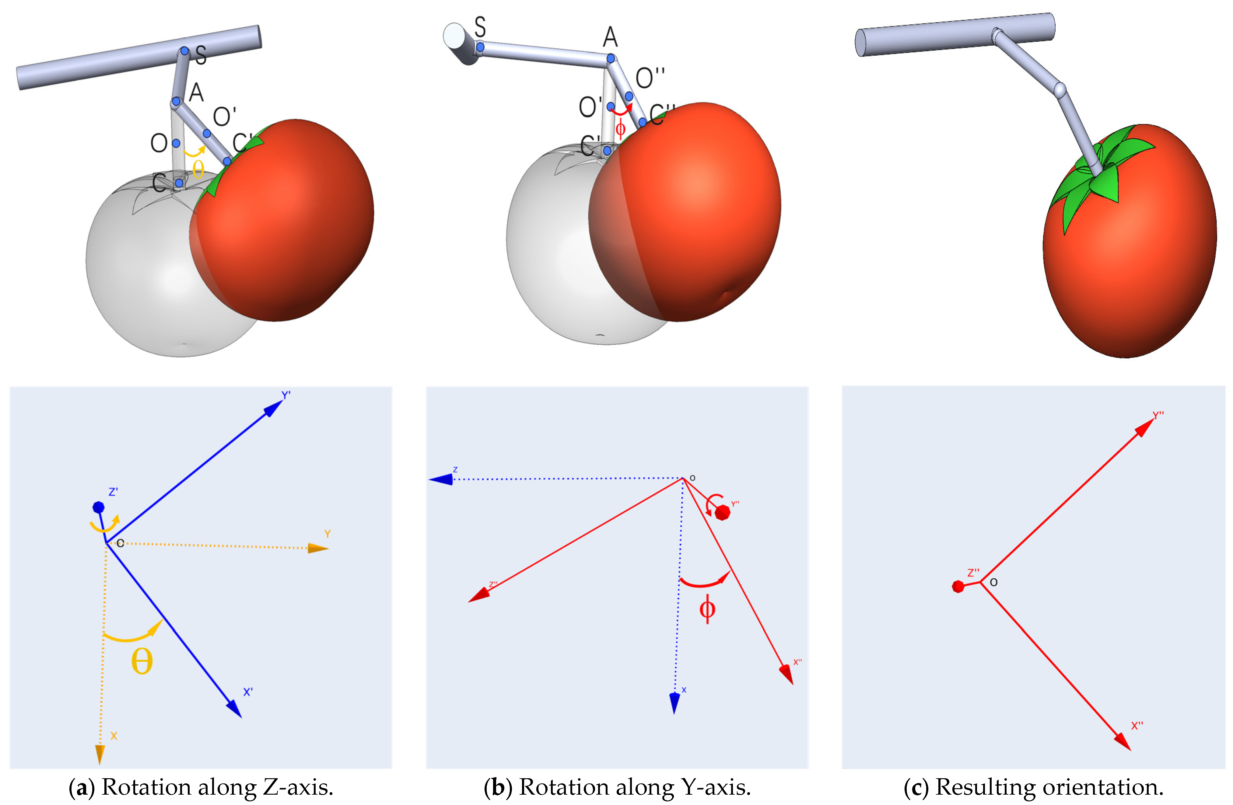
The pose of a tomato in 3D space has six degrees of freedom (DoF), including three positional coordinates (x, y, and z) and three rotational angles (θ, ϕ, and ω, corresponding to rotations along the Z-axis, X-axis, and Y-axis, respectively) [23]. ZYX Euler angles can be applied to represent the orientation of the tomato’s pose, as shown in Figure 7. The value of ω is set to zero, as we can generally assume that the fruit does not rotate along its axis [23] (since tomatoes are spherical). The cutting pose (CP) of the tomato can be formulated as follows:

$$\begin{array}{ll}{T}_{cp}={}_{O^{″}}{}^{O}R_{Z\prime Y\prime X\prime }(\theta ,\varphi )=R_{Z^{\prime }}(\theta )R_{Y^{\prime }}(\varphi )& =\left[\begin{array}{ccc}\cos \theta & -\sin \theta & 0\\ \sin \theta & \cos \theta & 0\\ 0& 0& 1\end{array}\right]\cdot \left[\begin{array}{ccc}\cos \varphi & 0& \sin \varphi \\ 0& 1& 0\\ -\sin \varphi & 0& \cos \varphi \end{array}\right]\\ & =\left[\begin{array}{ccc}\cos \theta \cos \varphi & -\sin \theta & \cos \theta \sin \varphi \\ \sin \theta \cos \varphi & \cos \theta & \sin \theta \sin \varphi \\ -\sin \varphi & 0& \cos \varphi \end{array}\right]\end{array}$$

(2)

where the parameter list [x, y, z, θ, ϕ] represents the fruit’s cutting pose.

2.7.1. Definition of the Pedicel Coordinate System

Based on the known 3D coordinates of keypoints A and C (Figure 7) at both ends of the pedicel in the camera coordinate system—($x_1,y_1,z_1$) and ($x_2,y_2,z_2$), respectively. The pedicel pose coordinate system can be defined as follows:

The CA vector represents the direction vector of the pedicel: ($x_1-x_2,y_1-y_2,z_1-z_2$). The unit vector of the pedicel’s direction vector (which serves as the Y-axis of the pedicel coordinate system) is computed as follows:

$$\widehat{Y}={\displaystyle \frac{\overrightarrow{CA}}{\left|\overrightarrow{CA}\right|}}$$

(3)

To determine the X-axis of the pedicel coordinate system, it is assumed that the Z-axis of the pedicel is coplanar with the Z-axis of the camera coordinate system (0, 0, 1). The X-axis can then be obtained by calculating the cross-product between the Z-axis of the camera coordinate system and the pedicel’s direction vector:

$$\widehat{X}=\widehat{Y}\times Z$$

(4)

The Z-axis of the pedicel coordinate system is determined by calculating the cross-product of the Y-axis and X-axis:

$$\widehat{Z}=\widehat{X}\times \widehat{Y}$$

(5)

2.7.2. Conversion from Pedicel Coordinate System to Camera Coordinate System

Three orthogonal unit vectors for the pedicel coordinate system are defined using the above steps. These unit vectors form the rotation matrix R, which represents the transformation from the pedicel coordinate system to the camera coordinate system. By extracting the Euler angles from this rotation matrix, the orientation of the pedicel in the camera coordinate system can be further described:

$$R=\left(\begin{array}{lll}{R}_{11}\hfill & R_{12}\hfill & R_{13}\hfill \\ R_{21}\hfill & R_{22}\hfill & R_{23}\hfill \\ R_{31}\hfill & R_{32}\hfill & R_{33}\hfill \end{array}\right)=\left(\begin{array}{ccc}{\widehat{X}}_x& {\widehat{Y}}_x& {\widehat{Z}}_x\\ {\widehat{X}}_y& {\widehat{Y}}_y& {\widehat{Z}}_y\\ {\widehat{X}}_z& {\widehat{Y}}_z& {\widehat{Z}}_z\end{array}\right)$$

(6)

2.7.3. Euler Angle Extraction in the Camera Coordinate System

The rotation angle ϕ around the X-axis is calculated as follows:

$$\varphi =\arctan 2\left(R_{32},R_{33}\right)=\arctan 2\left({\widehat{Y}}_z,{\widehat{Z}}_z\right)$$

(7)

The rotation angle θ around the Y-axis is calculated as follows:

$$\theta =\arctan 2\left(R_{21},R_{11}\right)=\arctan 2\left({\widehat{X}}_y,{\widehat{X}}_x\right)$$

(8)

2.7.4. Estimation of the Cutting Point Pose

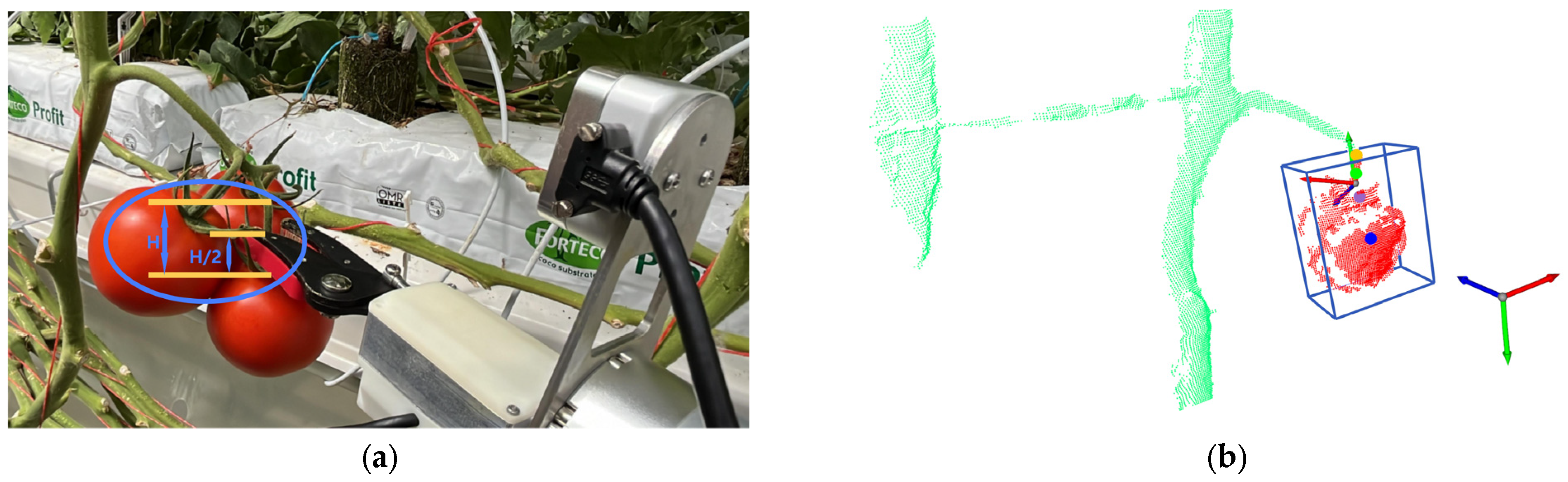
The cutting point is point O, at half of the AC vector (Figure 8a): O $\left({\displaystyle \frac{x_2-x_1}{2}},{\displaystyle \frac{y_2-y_1}{2}},{\displaystyle \frac{z_2-z_1}{2}}\right)$.

The pose of the tomato’s cutting point (Figure 8b) can be described as follows:

$$T_{cp}=\left[\begin{array}{cc}{}_{O^{″}}{}^{O}R_{Z\prime X\prime }(\theta ,\varphi )& O\\ 0& 1\end{array}\right]=\left[\begin{array}{cccc}\cos \theta \cos \varphi & -\sin \theta & \cos \theta \sin \varphi & {\displaystyle \frac{x_2-x_1}{2}}\\ \sin \theta \cos \varphi & \cos \theta & \sin \theta \sin \varphi & {\displaystyle \frac{y_2-y_1}{2}}\\ -\sin \varphi & 0& \cos \varphi & {\displaystyle \frac{z_2-z_1}{2}}\\ 0& 0& 0& 1\end{array}\right]$$

(9)

A geometric model is established to estimate the pedicel’s yaw and pitch angles. This estimation allows the robot to adaptively adjust its end-effector, ensuring that it grasps the pedicel at an optimal angle for cutting.

2.8. Experimental Environment and Parameter Settings

The experiments were conducted on a laptop (with an Intel^® Core™ i7-12700H processor, an NVIDIA^® GeForce RTX 3070Ti Laptop GPU, and 32 GB of RAM) for model training and testing. The software platform was based on the Windows 11 operating system, utilizing the PyTorch1.12.1 [24] deep learning framework and the MMPose [25] pose estimation framework. For training the pose estimation algorithm, the input images were resized to 256 × 192 pixels, and data augmentation strategies were employed to enhance the model’s robustness and prevent overfitting. Specifically, a random horizontal flipping (RandomFlip) augmentation was applied with a probability of 0.5 during training. This technique effectively doubled the dataset by creating mirrored versions of the images, helping the model become invariant to object orientation and improving its ability to generalize to unseen data.

The AdamW [26] optimizer was used with an initial learning rate of 0.0001 and a weight decay of 0.05. The training spanned 500 epochs, with a batch size of 16. A linear learning rate schedule was applied for the first 200 epochs, gradually increasing the learning rate, followed by a cosine annealing schedule [27] from the 200th to the 500th epoch. During training, weight files were saved every 50 epochs, and the best model was saved based on the PCK metric [28].

Additionally, dropout regularization was incorporated during training to prevent overfitting. Dropout was applied with a rate of 0.3, randomly deactivating 30% of the neurons in the network at each iteration, thereby reducing reliance on any single feature or path. Furthermore, weight decay (L2 regularization) was also applied through the AdamW optimizer to penalize large weights, further mitigating overfitting and encouraging the model to learn more generalizable features. Both techniques worked synergistically to enhance the model’s robustness and ability to generalize to unseen data.

3. Results

3.1. Evaluation Metrics for Keypoints Detection

In this experiment, the widely accepted percentage of correct keypoints (PCK) [28] metric was used to evaluate the accuracy of keypoint-based tomato pose estimation. The PCK metric assesses whether the distance between the predicted and ground-truth keypoints is within a predefined threshold α. The prediction is correct if the distance is smaller than this threshold. The calculation formula is as follows:

$$PCK@\alpha ={\displaystyle \frac{1}{N}}{\displaystyle {\sum }_{i=1}^{N}1}\left({\displaystyle \frac{{‖p_i-{\widehat{p}}_i‖}_2}{\mathrm{d}}}<\alpha \right)$$

(10)

where

N is the total number of keypoints;

$p_i$ is the ground-truth position of the i-th keypoint;

${\widehat{p}}_i$ is the predicted position of the i-th keypoint;

${‖p_i-{\widehat{p}}_i‖}_2$ is the Euclidean distance between the predicted and ground-truth positions;

d is a normalization factor, taken as the length of the tomato skeleton;

α is the threshold representing the acceptable maximum distance ratio;

1 is an indicator function that returns 1 if the condition inside is true and 0 otherwise.

3.2. Ablation Experiment

An ablation study was conducted to thoroughly analyze the model’s performance and evaluate the contribution and functionality of each component. As shown in

Table 3. Ablation study.

Model	Module					PCK@0.05 (%)	Inference Time (FPS)	FLOPs (G)	Parameters (M)
	Backbone		Neck	Head
	CSEFLayer		PDFN	StripPooling	SimCC
	CSPLayer	EFBlock
Baseline	√				√	72.44	125	0.876	5.814
A	√	√			√	74.95	129	0.886	5.884
B	√	√	√		√	78.21	110	4.313	29.914
C	√	√	√	√	√	82.51	100.78	5.122	31.015

, the RTMPose model was selected as the baseline to verify the advantages of the proposed TomatoPoseNet model. RTMPose employs CSPLayer as the backbone network and SimCC as the head network, offering strong real-time processing capabilities suitable for real-time tomato-picking tasks.

However, RTMPose has certain shortcomings in capturing detailed information, leading to deficiencies in detection accuracy. To address this issue, improved components were gradually integrated into the RTMPose model during the ablation experiments to validate their effectiveness on keypoint detection performance.

The EFBlock component was initially introduced into the baseline model to form Model A. After incorporating the EFBlock component (i.e., CSEFLayer), the PCK@0.05 increased from 72.44% to 74.95%, the inference speed improved from 125 FPS to 129 FPS, the number of FLOPs increased slightly from 0.876 G to 0.886 G, and the number of parameters rose from 5.184 M to 5.884 M. These results indicate that the CSEFLayer component significantly enhanced the model’s accuracy and inference speed, while the computational complexity and parameter count increases were minimal.

Subsequently, the PDFN component was added to Model A to obtain Model B. After adding the PDFN component, the PCK@0.05 increased further from 74.95% to 78.21%; however, the inference speed decreased from 129 FPS to 110 FPS, the number of FLOPs increased substantially from 0.886 G to 4.313 G, and the number of parameters grew from 5.884 M to 29.914 M. These results suggest that although the neck component improves the model’s accuracy, it also significantly increases the computational complexity and parameter count, thereby reducing the inference speed.

To further enhance the performance, both the PDFN and StripPooling components were integrated to form Model C. Incorporating the StripPooling component boosted PCK@0.05 to 82.51%, with a slight reduction in inference speed to 100.78 FPS, the number of FLOPs increasing to 5.122 G, and the number of parameters rising to 31.015 M. Despite the increased computational complexity, the StripPooling component effectively enhanced the detection accuracy. Consequently, Model C demonstrated the best performance, achieving significant accuracy improvements with a moderate increase in complexity and parameter count.

Considering that tomatoes are fragile fruits, the picking accuracy is particularly important. Inaccurate positioning may cause damage to the tomatoes, affecting the picking efficiency and fruit quality. Therefore, improving detection accuracy should be prioritized over inference speed and computational complexity in model selection. Based on these findings, Model C was chosen as the final configuration to achieve optimal performance.

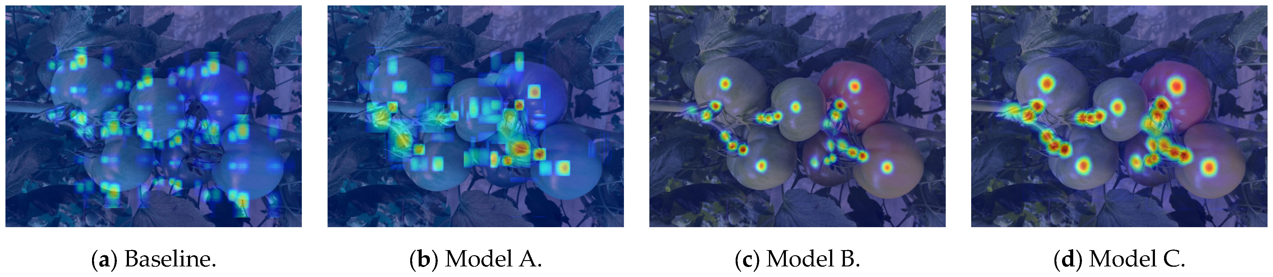
To validate the effectiveness of the proposed method, heatmap visualizations of the ablation experiment results are presented in Figure 9. From left to right, panel (a) represents the baseline model, while panels (b–d) correspond to models augmented with the CSEFLayer, PDFN, and StripPooling modules, respectively. The results demonstrate that, as each module is added, the model’s attention becomes more focused, with darker colors indicating higher confidence in the detected keypoints.

3.3. Comparison of the Performances of the Different Keypoint Detection Models

To validate the detection effectiveness of the proposed model, we compared it with several mainstream models in the field of pose estimation, including ViTPose [29], HRNet [20], Lite-HRNet [30], Hourglass [31], and RTMPose [32], using the same test set. The input image size for all models was set to 256 × 192 pixels, and the performance metrics are summarized in

Table 4. Comparison of the performance of different models.

Model	PCK@0.05 (%)	Inference Time (FPS)	FLOPs (G)	Parameters (M)
ViTPose	78.73	46.70	23.253	85.822
HRNet-w32	73.05	36.86	10.245	28.536
Lite-HRNet-30	71.51	22.97	0.546	1.763
Hourglass	73.37	38.45	28.639	94.845
RTMPose	72.44	125	0.876	5.814
TomatoPoseNet	82.51	100.78	5.122	31.015

.

As shown in Table 4, the proposed model achieves an excellent balance of keypoint accuracy (PCK@0.05), inference speed (FPS), computational complexity (FLOPs), and model parameter count (Parameters). Our model achieved the highest accuracy, with a PCK@0.05 of 82.51%, while maintaining a high inference speed of 100.78 FPS, significantly outperforming models such as ViTPose HRNet, Lite-HRNet, and Hourglass. Although the inference speed was slightly lower than that of RTMPose (125 FPS), our model demonstrated a notable 10.07% improvement in PCK@0.05 accuracy. Additionally, the model’s parameter count was 31.015 M, and its computational complexity was 5.122 G FLOPs, both of which are within reasonable limits and much lower than the parameter scale and computational load of models such as ViTPose, HRNet, and Hourglass.

Given the delicacy of tomatoes, where precise picking is essential to prevent damage and preserve quality, detection accuracy was prioritized over inference speed and computational complexity in our model selection. The proposed model embodies this emphasis on accuracy, achieving superior performance while maintaining acceptable speed and computational demands. These results demonstrate that the model offers a well-balanced trade-off between accuracy, speed, and complexity, highlighting significant advantages and practical value in pose estimation tasks.

To validate the accuracy of the proposed model for tomato pose estimation in complex orchard environments, we conducted five comparative experiments in real-world settings. Detailed results are provided in Figure 10.

In the first experiment, which focused on close-up views of mature tomatoes with visible stems and partial occlusion, only the proposed model successfully detected both the small tomato in the lower-right corner and the partially occluded tomato in the center. In the second experiment, which examined occluded mature tomatoes with partially visible stems, ViTPose exhibited a false detection for the central keypoints of the lower-right tomato, while our model maintained accurate predictions.

The third experiment assessed the models’ performance on mixed mature and immature tomatoes with visible stems. Except for our model, all other models failed to predict all of the keypoints of the four small tomatoes in the upper-left corner. The fourth experiment evaluated the models’ performance in handling mature tomatoes with severe occlusion. ViTPose and Lite-HRNet failed to detect keypoints in the central and lower-left regions, while HRNet, Hourglass, and RTMPose missed only the central keypoints. In contrast, our model accurately predicted all keypoints. The fifth experiment focused on detecting small, occluded, and overlapping tomatoes. Notably, our model was the only one to successfully detect the small tomatoes in the upper-right and lower-left corners, whereas the other models failed to detect all of them.

These results demonstrate that our proposed model offers superior accuracy and robustness in tomato pose estimation, particularly in handling occluded or small tomatoes. This performance, significantly surpassing that of other methods, highlights our model’s potential for practical applications in greenhouse environments.

3.4. Analysis of 6D Cutting Point Pose Estimation Results

To comprehensively evaluate the performance of the proposed 6D cutting point pose estimation algorithm in unstructured greenhouse environments, experiments were conducted on 30 different samples of tomato fruit. All experimental data were based on successful keypoint detections by the TomatoPoseNet model, demonstrating its effectiveness. The pedicels’ yaw angle (θ) and pitch angle (ϕ) were manually measured using an angle ruler and transformed from the camera coordinate system to the world coordinate system. This transformation allowed for a unified reference frame to quantitatively compare the algorithm’s predicted angles with the actual measured angles, thereby assessing the algorithm’s performance.

Table 5. Test results of cutting point pose estimation.

No.	L	R	F	B	Estimated Yaw Angle $\mathit{\theta }°$	Estimated Pitch Angle $\mathit{\phi }°$	Measured Yaw Angle $\mathit{\theta }°$	Measured Pitch Angle $\mathit{\phi }°$
1	√		√		21.7	20.9	25.6	16.87
2		√	√		22.3	16.8	22.1	20.49
3		√		√	29.78	18.5	33.86	18.27
4			√		0	20.3	4.1	23.33
5			√		0	15.5	0	18.43
6	√		√		13.7	9.7	11.62	6.22
7	√		√		10.6	16.4	9.12	19.87
8		√	√		10	17.4	7.65	20.77
9	√		√		36.5	14.4	38.53	13.27
10	√		√		9.6	13.4	5.82	13.01
11		√		√	7.6	15.7	3.8	18.29
12	√		√		25.4	14.1	30.23	16.15
13		√		√	15.6	8.9	11.92	4.28
14		√	√		11.8	9.5	10.57	14.14
15		√	√		33.42	30.5	30.98	27.27
16		√		√	15.6	8.9	11.92	4.28
17			√		0	28	0.95	22.30
18		√	√		9.64	15.53	4.59	12.69
19	√		√		30.52	17.44	26.49	11.57
20		√	√		31.22	10.01	27.68	5.03
21		√		√	12.45	13.21	8.96	8.42
22		√		√	9.34	16.54	4.32	11.48
23	√			√	32.14	8.96	31.95	7.28
24		√	√		14.65	15.47	10.26	11.34
25	√		√		8.24	24.12	7.68	20.17
26	√			√	9.41	34.26	5.25	30.92
27		√		√	35.49	30.16	38.72	27.56
28	√		√		8.41	17.41	3.03	12.65
29		√	√		10.41	13.46	8.44	16.34
30		√			32.19	10.50	28.15	16.60

presents the pose prediction and measurement results for the 30 tomato pedicel samples. In this study, the yaw angle was defined as positive when the pedicel was inclined to the left (L+, θ > 0) and negative when inclined to the right (L−, θ < 0). Similarly, the pitch angle was defined as positive when inclined forward (F+, ϕ > 0) and negative when inclined backward (B−, ϕ < 0) [8]. Figure 7 illustrates the definitions of θ and ϕ. Although the manual measurement process may introduce some systematic errors, comparing the objectively measured angles with the predicted angles still provides a reliable evaluation of the proposed pose estimation algorithm’s performance.

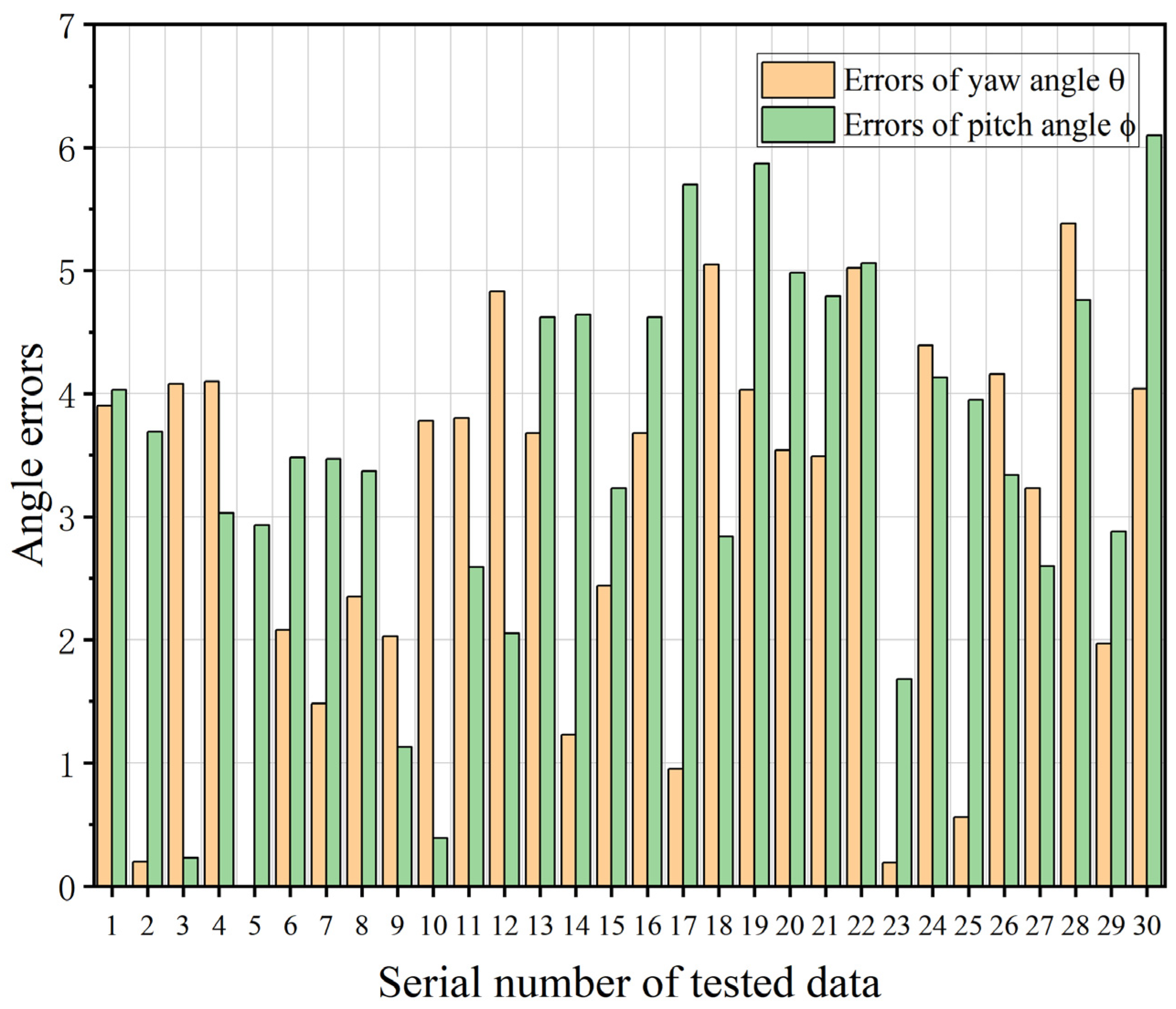
During the data preprocessing stage, special attention was paid to exclude potential errors caused by missing data in the point cloud images, ensuring the reliability of the pose estimation results. The prediction error distributions for the 30 sets of tomato pedicels were obtained by analyzing the pose predictions for the yaw angle and pitch angle, as shown in Figure 11.

To quantitatively evaluate the accuracy of the pose estimation algorithm, the mean absolute error (MAE) and maximum error (MaxE) were employed as evaluation metrics, defined as follows:

$$\begin{array}{c}MA{E}_{\theta }={\displaystyle \frac{1}{N}}{\displaystyle \sum _{i=1}^N\left|{\theta }_i-{\widehat{\theta }}_{\mathrm{i}}\right|},MAx{E}_{\theta }={\displaystyle \frac{1}{N}}\underset{1\le i\le N}{\max }\left|{\theta }_i-{\widehat{\theta }}_i\right|\\ MA{E}_{\varphi }={\displaystyle \frac{1}{N}}{\displaystyle \sum _{i=1}^N\left|{\varphi }_i-{\widehat{\varphi }}_i\right|},MAx{E}_{\varphi }={\displaystyle \frac{1}{N}}\underset{1\le i\le N}{\max }\left|{\varphi }_i-{\widehat{\varphi }}_i\right|\end{array}$$

(11)

where N represents the total number of test samples; ${\theta }_i$ and ${\varphi }_i$ are the actual measured yaw and pitch angles of the i-th sample, respectively; and ${\widehat{\theta }}_i$ and ${\widehat{\varphi }}_i$ are the corresponding predicted angles.

Based on the experimental data, the proposed pose estimation algorithm achieved an MAE of 2.98° and a MaxE of 5.38° for the yaw angle (θ), and an MAE of 3.54° and a MaxE of 6.10° for the pitch angle (ϕ). These quantitative results indicate that the algorithm can accurately predict the 6D pose of tomato cutting points in unstructured greenhouse environments, with average errors controlled within 3.6° and maximum errors within 6.5°, meeting the practical requirements of tomato-harvesting robots.

4. Discussion

The TomatoPoseNet model proposed in this study demonstrates exceptional performance in keypoint detection tasks, striking a balance between accuracy and speed. Compared to existing mainstream pose estimation models, TomatoPoseNet achieves a superior accuracy of 82.51% on the PCK@0.05 metric while maintaining an inference speed of 100.78 FPS. This performance underscores the model’s high accuracy and real-time capability.

In five comparative experiments conducted in real-world greenhouse environments, TomatoPoseNet exhibited outstanding detection capabilities for occluded or small tomato targets. While other models frequently misidentified or failed to detect partially occluded or overlapping tomatoes, TomatoPoseNet accurately detected all keypoints. This remarkable performance highlights the model’s robustness and reliability in complex environments, providing a solid technological foundation for automated greenhouse applications.

The 6D cutting point pose estimation algorithm [33,34,35] underwent a comprehensive evaluation using 30 distinct tomato samples. The results indicate that the algorithm can accurately predict the 6D pose of tomato cutting points in unstructured greenhouse environments, with average errors below 3.6° and maximum errors within 6.5°. These results meet the practical requirements of tomato-harvesting robots, demonstrating the algorithm’s potential for real-world applications.

Overall, the TomatoPoseNet model combines high robustness with real-time performance and is easily deployable on embedded devices. This combination of features presents significant opportunities for enhancing automation levels and efficiency in greenhouse tomato harvesting. However, it is essential to note that the model’s generalization capability across different tomato varieties and environmental conditions requires further validation. Additionally, the manual angle measurement process may introduce systematic errors, necessitating the adoption of more precise measurement techniques in future research.

Based on these findings, we propose the following directions for future research:

• Diversifying the datasets: Developing a more extensive and diverse tomato dataset encompassing various lighting conditions, tomato varieties, and greenhouse environments could be beneficial. Collecting data under different illumination scenarios may improve the model’s performance consistency despite variations in lighting. Additionally, integrating multi-sensor data and applying advanced image processing techniques can enhance performance by compensating for lighting inconsistencies.
• Exploring advanced depth-sensing technologies: Advanced depth-sensing methods, such as triangulation depth techniques or multi-line LiDAR with RGB cameras, should be investigated to obtain more comprehensive point cloud information.
• Extending model applicability to other crops: The model’s applicability could be expanded to detect and estimate the pose of other fruits and vegetables, further validating its versatility and practical value in intelligent agriculture.
• Enhancing the model’s robustness to environmental variations: Methods should be explored to improve the model’s adaptability to unexpected environmental changes, such as wind-induced movements of tomatoes, by incorporating temporal information or utilizing more robust feature extraction techniques.
• Addressing practical deployment challenges: Integrating the algorithm with various hardware and software components to develop a complete robotic system will be necessary. This integration will require careful design and debugging of the robotic control, navigation, and communication systems to ensure stability and reliability. Future research will involve deploying TomatoPoseNet across different devices and conducting large-scale field trials, allowing for ongoing improvements and iterations.

These future research directions address the current limitations of this study while building upon its significant contributions to automated greenhouse harvesting technology. By pursuing these avenues, we can further improve the model’s performance and broaden its applicability.

5. Conclusions

In this study, TomatoPoseNet, a novel keypoint-based pose estimation model, was developed to accurately detect the 6D spatial pose of tomatoes, fulfilling agronomic requirements for non-destructive harvesting. TomatoPoseNet comprises three main components: a CSEFLayer backbone network, a parallel deep fusion network (PDFN) neck, and a SimCC head network.

The CSEFLayer, based on the CSPLayer design, efficiently fuses multiscale features while maintaining computational efficiency. The PDFN enhances feature representation by integrating features from multiple parallel branches. The head network employs SimCC for keypoint detection; it incorporates a StripPooling module, which improves the model’s ability to capture features of different scales and shapes through horizontal and vertical strip pooling.

TomatoPoseNet demonstrated exceptional performance in both keypoint detection and 6D pose estimation tasks. The average precision for keypoint detection (PCK@0.05) reached 82.51%, surpassing those of ViTPose, HRNet, Lite-HRNet, Hourglass, and RTMPose by 3.78%, 9.46%, 11%, 9.14%, and 10.07%, respectively. The model achieved an inference speed of 100.78 FPS, combining high accuracy with real-time performance and significantly outperforming existing mainstream models.

TomatoPoseNet exhibited superior capabilities in handling occlusions and detecting small targets in complex greenhouse environments, providing a solid technical foundation for practical applications. The 6D pose estimation algorithm, based on 3D keypoint information, achieved high-precision predictions; the mean absolute errors for the yaw and pitch angles of the cutting points were 2.98° and 3.54°, respectively, with the maximum errors contained within 6.5°. These results validate the algorithm’s effectiveness and reliability in unstructured greenhouse settings.

In conclusion, TomatoPoseNet offers significant advantages in its high accuracy, real-time performance, and ease of deployment on embedded devices; it provides an effective solution for the 6D cutting point pose estimation of tomatoes, meeting the agronomic requirements for non-destructive harvesting.

References

- Rong, J.; Zheng, W.; Qi, Z.; Yuan, T.; Wang, P. RTMFusion: An Enhanced Dual-Stream Architecture Algorithm Fusing RGB and Depth Features for Instance Segmentation of Tomato Organs. Measurement 2025, 239, 115484. [Google Scholar] [CrossRef]
- Rong, J.; Hu, L.; Zhou, H.; Dai, G.; Yuan, T.; Wang, P. A Selective Harvesting Robot for Cherry Tomatoes: Design, Development, Field Evaluation Analysis. J. Field Robot. 2024, 41, 2564–2582. [Google Scholar] [CrossRef]
- Zhao, Y.; Gong, L.; Huang, Y.; Liu, C. A Review of Key Techniques of Vision-Based Control for Harvesting Robot. Comput. Electron. Agric. 2016, 127, 311–323. [Google Scholar] [CrossRef]
- Huang, M.-L.; Wu, Y.-S. GCS-YOLOV4-Tiny: A Lightweight Group Convolution Network for Multi-Stage Fruit Detection. Math. Biosci. Eng. 2022, 20, 241–268. [Google Scholar] [CrossRef]
- Wang, X.; Wu, Z.; Jia, M.; Xu, T.; Pan, C.; Qi, X.; Zhao, M. Lightweight SM-YOLOv5 Tomato Fruit Detection Algorithm for Plant Factory. Sensors 2023, 23, 3336. [Google Scholar] [CrossRef]
- Yang, G.; Wang, J.; Nie, Z.; Yang, H.; Yu, S. A Lightweight YOLOv8 Tomato Detection Algorithm Combining Feature Enhancement and Attention. Agronomy 2023, 13, 1824. [Google Scholar] [CrossRef]
- Guo, N.; Zhang, B.; Zhou, J.; Zhan, K.; Lai, S. Pose Estimation and Adaptable Grasp Configuration with Point Cloud Registration and Geometry Understanding for Fruit Grasp Planning. Comput. Electron. Agric. 2020, 179, 105818. [Google Scholar] [CrossRef]
- Rong, J.; Dai, G.; Wang, P. A Peduncle Detection Method of Tomato for Autonomous Harvesting. Complex Intell. Syst. 2022, 8, 2955–2969. [Google Scholar] [CrossRef]
- Zhong, Z.; Xiong, J.; Zheng, Z.; Liu, B.; Liao, S.; Huo, Z.; Yang, Z. A Method for Litchi Picking Points Calculation in Natural Environment Based on Main Fruit Bearing Branch Detection. Comput. Electron. Agric. 2021, 189, 106398. [Google Scholar] [CrossRef]
- Cao, Z.; Simon, T.; Wei, S.-E.; Sheikh, Y. Realtime Multi-Person 2D Pose Estimation Using Part Affinity Fields. In Proceedings of the 2017 IEEE Conference on Computer Vision and Pattern Recognition (CVPR), Honolulu, HI, USA, 21–26 July 2017; pp. 1302–1310. [Google Scholar]
- Zhang, F.; Gao, J.; Zhou, H.; Zhang, J.; Zou, K.; Yuan, T. Three-Dimensional Pose Detection Method Based on Keypoints Detection Network for Tomato Bunch. Comput. Electron. Agric. 2022, 195, 106824. [Google Scholar] [CrossRef]
- Jiang, T.; Li, Y.; Feng, H.; Wu, J.; Sun, W.; Ruan, Y. Research on a Trellis Grape Stem Recognition Method Based on YOLOv8n-GP. Agriculture 2024, 14, 1449. [Google Scholar] [CrossRef]
- Kim, T.; Lee, D.-H.; Kim, K.-C.; Kim, Y.-J. 2D Pose Estimation of Multiple Tomato Fruit-Bearing Systems for Robotic Harvesting. Comput. Electron. Agric. 2023, 211, 108004. [Google Scholar] [CrossRef]
- Zhang, F.; Gao, J.; Song, C.; Zhou, H.; Zou, K.; Xie, J.; Yuan, T.; Zhang, J. TPMv2: An End-to-End Tomato Pose Method Based on 3D Key Points Detection. Comput. Electron. Agric. 2023, 210, 107878. [Google Scholar] [CrossRef]
- Ci, J.; Wang, X.; Rapado-Rincón, D.; Burusa, A.K.; Kootstra, G. 3D Pose Estimation of Tomato Peduncle Nodes Using Deep Keypoint Detection and Point Cloud. Biosyst. Eng. 2024, 243, 57–69. [Google Scholar] [CrossRef]
- Liu, J.; Peng, Y.; Faheem, M. Experimental and Theoretical Analysis of Fruit Plucking Patterns for Robotic Tomato Harvesting. Comput. Electron. Agric. 2020, 173, 105330. [Google Scholar] [CrossRef]
- Lyu, C.; Zhang, W.; Huang, H.; Zhou, Y.; Wang, Y.; Liu, Y.; Zhang, S.; Chen, K. RTMDet: An Empirical Study of Designing Real-Time Object Detectors. arXiv 2022, arXiv:2212.07784. [Google Scholar]
- Li, Y.; Yang, S.; Liu, P.; Zhang, S.; Wang, Y.; Wang, Z.; Yang, W.; Xia, S.-T. SimCC: A Simple Coordinate Classification Perspective for Human Pose Estimation. In Computer Vision—ECCV 2022; Avidan, S., Brostow, G., Cissé, M., Farinella, G.M., Hassner, T., Eds.; Lecture Notes in Computer Science; Springer Nature: Cham, Switzerland, 2022; Volume 13666, pp. 89–106. ISBN 978-3-031-20067-0. [Google Scholar]
- Krizhevsky, A.; Sutskever, I.; Hinton, G.E. ImageNet Classification with Deep Convolutional Neural Networks. Commun. ACM 2017, 60, 84–90. [Google Scholar] [CrossRef]
- Sun, K.; Xiao, B.; Liu, D.; Wang, J. Deep High-Resolution Representation Learning for Human Pose Estimation. In Proceedings of the 2019 IEEE/CVF Conference on Computer Vision and Pattern Recognition (CVPR), Long Beach, CA, USA, 15–20 June 2019; pp. 5686–5696. [Google Scholar]
- Hong, Y.; Pan, H.; Sun, W.; Jia, Y. Deep Dual-Resolution Networks for Real-Time and Accurate Semantic Segmentation of Road Scenes. arXiv 2021, arXiv:2101.06085. [Google Scholar]
- Hou, Q.; Zhang, L.; Cheng, M.-M.; Feng, J. Strip Pooling: Rethinking Spatial Pooling for Scene Parsing. In Proceedings of the 2020 IEEE/CVF Conference on Computer Vision and Pattern Recognition (CVPR), Seattle, WA, USA, 13–19 June 2020; pp. 4002–4011. [Google Scholar]
- Kang, H.; Chen, C. Real-Time Fruit Recognition and Grasping Estimation for Autonomous Apple Harvesting. Sensors 2019, 19, 4599. [Google Scholar] [CrossRef]
- Paszke, A.; Gross, S.; Massa, F.; Lerer, A.; Bradbury, J.; Chanan, G.; Killeen, T.; Lin, Z.; Gimelshein, N.; Antiga, L.; et al. PyTorch: An Imperative Style, High-Performance Deep Learning Library. arXiv 2019, arXiv:1912.01703. [Google Scholar]
- MMPose Contributors. Openmmlab Pose Estimation Toolbox and Benchmark. 2020. Available online: https://github.com/open-mmlab/mmpose (accessed on 25 April 2024).
- Loshchilov, I.; Hutter, F. Decoupled Weight Decay Regularization. arXiv 2017, arXiv:1711.05101. [Google Scholar]
- Loshchilov, I.; Hutter, F. SGDR: Stochastic Gradient Descent with Warm Restarts. arXiv 2016, arXiv:1608.03983. [Google Scholar]
- Yang, Y.; Ramanan, D. Articulated Human Detection with Flexible Mixtures of Parts. IEEE Trans. Pattern Anal. Mach. Intell. 2013, 35, 2878–2890. [Google Scholar] [CrossRef] [PubMed]
- Xu, Y.; Zhang, J.; Zhang, Q.; Tao, D. ViTPose: Simple Vision Transformer Baselines for Human Pose Estimation. Adv. Neural Inf. Process. Syst. 2022, 35, 38571–38584. [Google Scholar]
- Yu, C.; Xiao, B.; Gao, C.; Yuan, L.; Zhang, L.; Sang, N.; Wang, J. Lite-HRNet: A Lightweight High-Resolution Network. In Proceedings of the 2021 IEEE/CVF Conference on Computer Vision and Pattern Recognition (CVPR), Nashville, TN, USA, 20–25 June 2021; pp. 10435–10445. [Google Scholar]
- Newell, A.; Yang, K.; Deng, J. Stacked Hourglass Networks for Human Pose Estimation. arXiv 2016, arXiv:1603.06937. [Google Scholar]
- Jiang, T.; Lu, P.; Zhang, L.; Ma, N.; Han, R.; Lyu, C.; Li, Y.; Chen, K. RTMPose: Real-Time Multi-Person Pose Estimation Based on MMPose. arXiv 2023, arXiv:2303.07399. [Google Scholar]
- Xu, H.; Li, Q.; Chen, J. Highlight Removal from A Single Grayscale Image Using Attentive GAN. Appl. Artif. Intell. 2022, 36, 1988441. [Google Scholar] [CrossRef]
- Sun, J.; Zhou, L.; Geng, B.; Zhang, Y.; Li, Y. Leg State Estimation for Quadruped Robot by Using Probabilistic Model with Proprioceptive Feedback. IEEE ASME Trans. Mechatron. 2024, 1–12. [Google Scholar] [CrossRef]
- Wang, K.; Boonpratatong, A.; Chen, W.; Ren, L.; Wei, G.; Qian, Z.; Lu, X.; Zhao, D. The Fundamental Property of Human Leg During Walking: Linearity and Nonlinearity. IEEE Trans. Neural Syst. Rehabil. Eng. 2023, 31, 4871–4881. [Google Scholar] [CrossRef]
Figure 1.
Data collection of tomato fruit–stem structure and different poses: (a) Data collection setup in a greenhouse using a robotic system for tomato picking. (b) Structure of the tomato fruit-bearing system, showing key components such as the main stem, branch, peduncle, pedicel, and fruit axis. (c) Tomato leaning to the left. (d) Tomato leaning to the right. (e) Tomato leaning forward. (f) Tomato leaning backward. (g) Strong light. (h) Natural light. (i) Low light.
Figure 2.
(a) Pose of the tomato fruit-bearing system using 4 keypoints and their sequential paring (the keypoints and parts are color-coded: fruit center = blue, calyx = orange, abscission = red, and branch point = yellow). (b) Annotation of tomato target and its 4 keypoints for training (The target bounding box for the tomato is represented in green).