Modeling Airflow and Temperature in a Sealed Cold Storage System for Medicinal Plant Cultivation Using Computational Fluid Dynamics (CFD)

Abstract

Effective air circulation is crucial for plant growth, requiring adequate airflow and environmental stability. This study utilized Computational Fluid Dynamics (CFD) to analyze airflow patterns in a controlled testing chamber, focusing on how miniature fan placement affects airflow direction and temperature distribution. Ten case studies were conducted, with the CFD model validated against experimental data collected from six monitoring locations on the plant growth table. Model validation was performed using statistical analyses including coefficient of determination (R²), root mean square error (RMSE), and mean absolute error (MAE). The validation results showed strong agreement between simulated and experimental data, with R² values of 0.92 for temperature and 0.89 for airflow velocity. Statistical analysis showed significant differences in both airflow and temperature models at the 0.05 level, with the CFD model validation yielding an RMSE of 2.02 and an average absolute error of 1.17. Among the tested configurations, case M1 achieved the highest air velocity (0.317 m/s) and lowest temperature (27.03 °C), compared to M2 (0.255 m/s, 27.17 °C) and M3 (0.164 m/s, 27.18 °C). The temperature variations between cases significantly impacted cold storage efficiency, with case M1’s superior airflow distribution providing more uniform cooling. These findings offer practical guidelines for optimizing ventilation system design in medicinal plant cultivation facilities, particularly in maintaining ideal storage conditions through strategic fan placement and airflow management.

1. Introduction

Indoor plant factories represent state-of-the-art enclosed growth systems characterized by multi-tiered production racks and advanced lighting control mechanisms. In comparison to traditional greenhouses, these facilities exhibit markedly higher efficiency in water utilization, carbon dioxide management, and land resource optimization [1]. These meticulously controlled environments, augmented by cutting-edge sensor networks and artificial intelligence systems, facilitate optimal plant growth and development through precise regulation of pivotal parameters, encompassing light intensity, temperature, humidity, CO₂ levels, and nutrient availability. This holistic optimization strategy expedites flowering periods while considerably reducing breeding cycle duration [2,3].

Computational Fluid Dynamics (CFD) emerges as an indispensable tool in contemporary greenhouse management, enabling comprehensive environmental analysis and underpinning the development of automated control systems that enhance resource efficiency and mitigate greenhouse gas emissions [4,5,6]. The present research endeavor concentrates on flow field simulation and the optimization of cultivation racks and vertical farms, harnessing CFD techniques to scrutinize airflow patterns, temperature distribution, and gas dispersion within regulated agricultural environments. These factors are paramount in establishing uniform growth conditions and nurturing robust plant development.

Furthermore, the assimilation of advanced technologies, such as cloud computing and machine learning, has ushered in a revolution in greenhouse management, empowered by real-time monitoring capabilities and intricate decision support systems [7,8,9]. In tandem with sophisticated transient modeling techniques that permit accurate climate prediction and control with minimal data input [10], the deployment of CFD in synergy with these innovations will forge an efficacious framework for bolstering the efficiency and sustainability of vertical farming systems.

Closed cultivation systems, epitomized by hydroponic technologies, symbolize a momentous stride forward in environmental control, particularly in confronting the challenges posed by climate change and the burgeoning demand for sustainable agriculture [11,12]. These systems efficaciously surmount the constraints of conventional open-field farming, such as weather variability and pest pressure, while concomitantly contributing to global food security.

Advanced imaging technologies, including Near-Infrared (NIR) and Infrared Thermography (INRT), demonstrate significant potential for enhancing plant development, optimizing greenhouse cultivation systems, and improving temperature control in climate management applications [13,14]. Concurrent innovations in electrical acceleration technology, particularly nanorhodium-iridium sheets, present promising sustainable energy solutions for indoor agriculture through enhanced hydrogen evolution in water separation systems [15]. Furthermore, advanced materials such as defective nanorods incorporating Metal-Organic Frameworks (MOFs), specifically MIL-88B, contribute to improved indoor air quality by effectively oxidizing formaldehyde, thereby creating healthier environments for both plant and human occupants [16].

Enclosed growing chambers play a fundamental role in future plant cultivation practices, as these controlled environments effectively mitigate external stressors, particularly those associated with climate change, that can adversely affect plant heat stress responses [17,18,19,20]. The management of environmental factors controlling both biotic and abiotic stresses has become increasingly critical for optimizing agricultural yields, especially given the challenges posed by climate change, geographical constraints, and global uncertainties [21,22,23].

The regulation of air quality in confined agricultural spaces plays a crucial role in maintaining ecosystem dynamics, regulating terrestrial carbon cycles, and managing carbon transfer between terrestrial and aquatic systems [24]. Additionally, enclosed agricultural facilities serve as vital repositories for plant genetic diversity, enhancing resilience to environmental perturbations and maintaining ecological stability in the face of global environmental changes [25].

The primary objective of this research is to develop a Computational Fluid Dynamics (CFD) model for a vertical farming system, with emphasis on optimizing air distribution and temperature uniformity within the cultivation chamber. Effective environmental control not only reduces operational costs but also enhances overall system performance. The chamber design incorporates strategic fan placement to evaluate its impact on airflow patterns and temperature distribution throughout the growing space. The study focuses on examining how various fan positions influence air circulation patterns and temperature gradients across the cultivation area, aiming to identify optimal configurations that create uniform environmental conditions essential for consistent plant development. Through the strategic management of airflow patterns and temperature distribution, this research seeks to establish guidelines for creating optimal growing conditions in vertical farming systems, ultimately enhancing cultivation efficiency and crop uniformity.

2. Materials and Methods

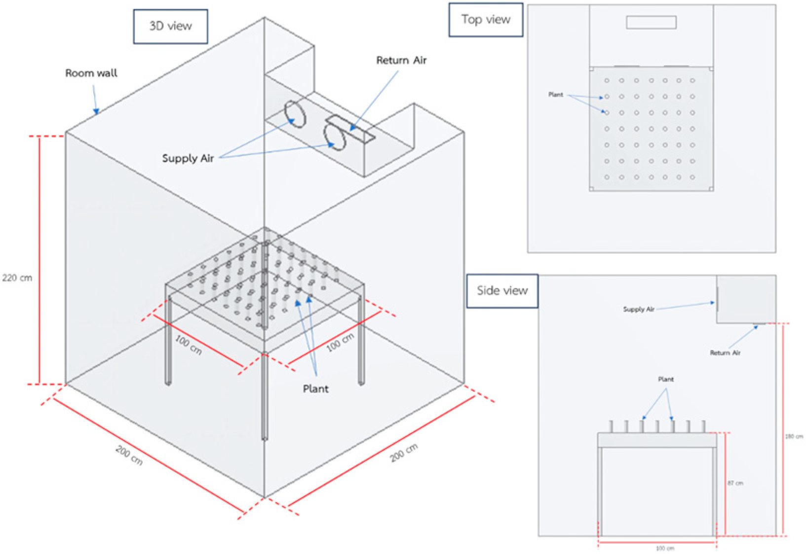
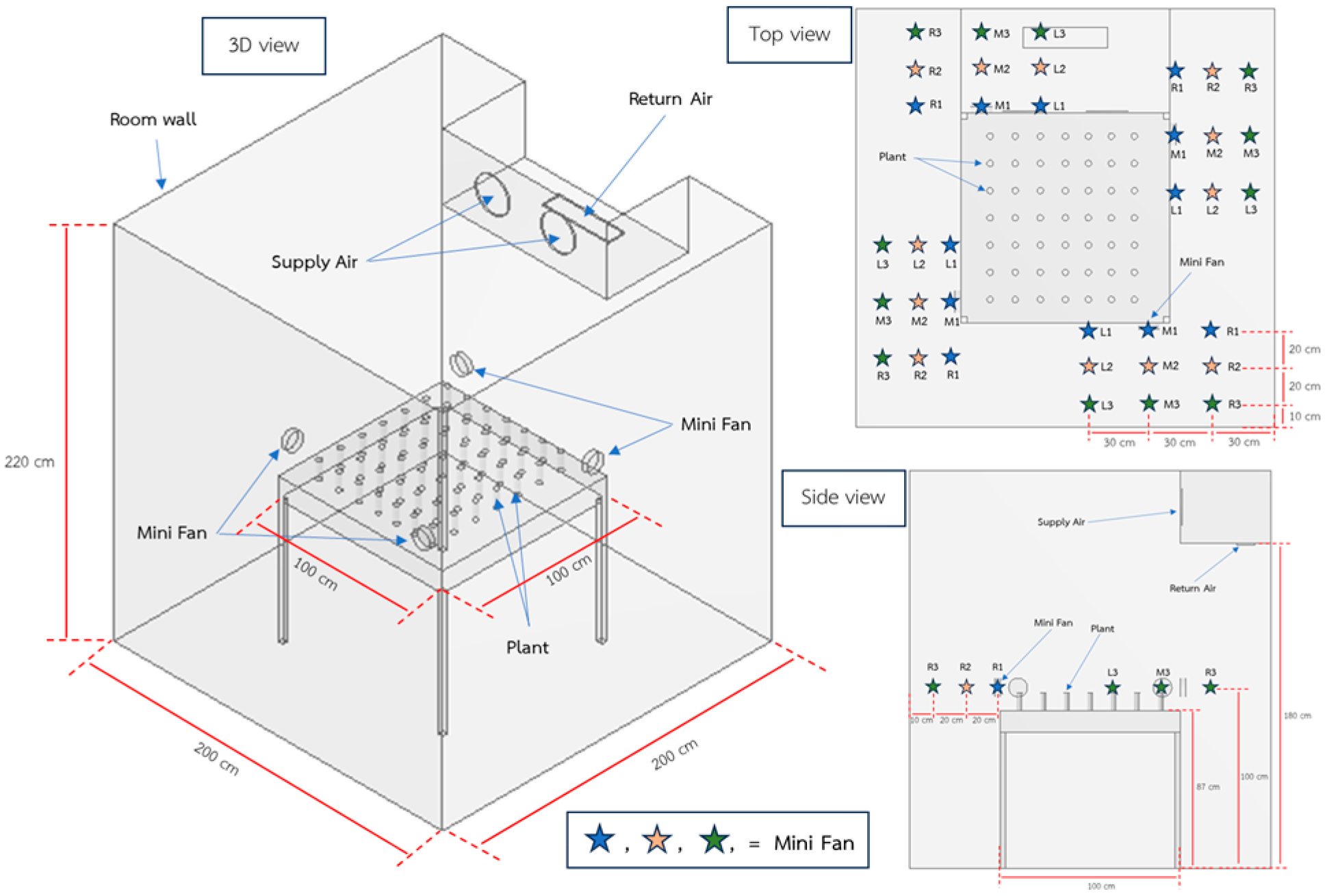
2.1. Case Description

A specialized testing facility has been established at the Centre for Agricultural Mechanical Research and Post-Harvest Sciences, Khon Kaen University, Thailand, to investigate air circulation dynamics and optimize the distribution of air and carbon dioxide (CO₂)—crucial elements for plant growth enhancement. The experimental chamber comprises a climate-controlled room measuring 2 m in length, 2 m in width, and 2.2 m in height, equipped with air conditioning systems to maintain precise environmental conditions. Within this chamber, a custom-designed planting table (87 cm in height, 1 m in width, and 1 m in length) serves as the primary experimental platform (Figure 1).

The research methodology encompasses ten distinct experimental scenarios, beginning with a control condition without ventilation. Subsequently, nine additional configurations are tested using a compact fan positioned according to a systematic grid layout divided into three segments. The experimental design prioritizes corner placement of the fan, as preliminary studies indicate superior airflow effectiveness compared to alternative positions. Throughout all trials, the fan operates at a constant velocity of 1 m per second, directing airflow to predetermined points as illustrated in Figure 2.

The experimental planting table incorporates four adjustable angular positions to facilitate optimal air supply installation and enhance airflow dynamics. The selection of a compact fan operating at a moderate velocity (1 m/s) represents a carefully balanced approach, providing sufficient ventilation while avoiding potential plant damage from excessive air speeds or turbulence. This controlled ventilation system plays a crucial role in maintaining optimal temperature, humidity, and CO₂ levels—environmental parameters essential for robust plant development.

2.2. CFD Simulation

2.2.1. Computational Fluid Dynamics Model

Computational Fluid Dynamics (CFD) has undergone substantial evolution since its inception, transforming from pioneering individual contributions into a sophisticated and widely adopted analytical tool across multiple industries. Modern CFD solutions integrate complex mathematical principles, physical models, numerical methodologies, intuitive user interfaces, and advanced visualization techniques, enabling precise numerical representation of diverse fluid flow phenomena [26]. This comprehensive integration has established CFD as an indispensable instrument in engineering applications.

The expanding adoption of CFD technology among researchers has facilitated detailed evaluation of air quality in various agricultural environments, including greenhouses, livestock facilities, and feed storage units. This application has proven particularly valuable in optimizing indoor environmental conditions through systematic design approaches [27]. The CFD modeling and simulation process requires rigorous validation of numerical results to ensure accuracy, typically achieved through experimental quantification of environmental parameters within the studied structure.

Among available CFD software v 19.1 platforms, Ansys Fluent has emerged as a leading solution, distinguished by its capability to independently evaluate and resolve airflow behavior through sophisticated quantitative constraint techniques. Contemporary simulations predominantly operate under static conditions, with many investigations employing the Standard k-ε model to determine ventilation rates and analyze temperature distribution patterns within plant environments [28].

The CFD analysis methodology facilitates controlled synthesis through the Finite Volume Method (FVM), with model development typically proceeding through three distinct phases, as follows:

Preprocessing Establishment of the computational framework and boundary conditions.

Processing Implementation of the finite volume method and numerical calculations.

Postprocessing Analysis and visualization of computational results.

2.2.2. Regulatory Equation

Computational Fluid Dynamics (CFD) is utilized to predict the direction of airflow, allowing for visualization in three dimensions within the refrigerator. FLUENT employs a finite volume method with a cell-centered formulation, utilizing principles of momentum and energy conservation. The general governing equations of CFD can be represented as follows [29]

$$\nabla ·\left(\rho \mu \theta -\tau \nabla \varnothing \right)=s$$

(1)

In this context, $\rho$ denotes fluid density, while $\varnothing$ represents the variable under investigation, which includes continuity, momentum, energy, k, and $\epsilon$. $\mu$ The symbol μ is utilized to signify fluid viscosity, and. $\tau$ denotes the diffusion coefficient, whereas $S$ represents the source term. For the purposes of this study, the interior of the farm is treated as homogeneous, with a substantial influx of water vapor (kg m⁻³ s⁻¹) and a consistent energy source (W m⁻³)

The computational fluid dynamics (CFD) simulation addresses the flow dynamics of fluids within the greenhouse environment. The Navier–Stokes equations are derived from the application of Newton’s second law to the motion of fluid elements [30].

$${\displaystyle \frac{\partial \rho \overrightarrow{U}}{\partial x}}+\overrightarrow{U}\nabla \rho \overrightarrow{U}=-\nabla p+\mu {\nabla }^2\overrightarrow{U}+S_U$$

(2)

In this context, $\rho$ represents fluid density, and $\overrightarrow{U}$ signifies the velocity vector, with its x-component denoted as $u,p$ indicates pressure, $\mu$ represents turbulent dynamic viscosity, and $S_U$ refers to the momentum source.

The model incorporates the Navier–Stokes equations, which are solved using a realizable turbulence model to enhance accuracy. This turbulence approach provides a more precise distribution of airflow fields compared to conventional turbulence models.

$${\displaystyle \frac{\partial \rho }{\partial t}}+\nabla (\rho \overrightarrow{v})=0$$

(3)

where $\rho$ is the density, t represents the time, and $\overrightarrow{v}$ is the velocity vector.

$${\displaystyle \frac{\partial }{\partial t}}(\rho \overrightarrow{v})+\nabla (\rho \overrightarrow{v}\overrightarrow{v})=-\nabla P+\nabla \cdot (\overline{\overline{\tau }})+\rho \overrightarrow{g}$$

(4)

In this equation, $P$ is defined as pressure, $\overline{\overline{\tau }}$ as the stress tensor, and $\overrightarrow{g}$ as gravitational acceleration.

2.3. Establishment of Experimental Parameters for Computational Fluid Dynamics Simulation

The parameters used in the Computational Fluid Dynamics (CFD) simulation are derived from empirical data obtained in the laboratory setting. The external temperature is determined based on the prevailing environmental conditions. The wind speed is established by the rotational velocity of the air fan, which is measured at 1 m/s, corresponding to the average flow rate. The validity of the CFD model is evaluated by comparing temperature measurements from six distinct locations within the experimental setup. This research employs the standard k-ε model, recognizing that precise modeling is crucial for the accuracy and reliability of the simulation results (

Table 1. Preliminary Assumptions Used in the Analysis.

Order	Assumption
1	The analysis is static (steady state).
2	Use the properties of air as flow characteristics in the analysis.
3	Three-dimensional analysis.
4	An analysis of the gravitational aggregation of the Earth.
5	The viscosity model employs the standard k-epsilon equation
6	The model represents a refrigerator, and the walls of the chamber are insulated.

).

This research aims to investigate the impact of small fan placement within a testing environment, which is a crucial factor in enhancing air circulation and the efficiency of heat removal and air distribution. In this study, the boundary conditions of the fan were specified using the exit velocity as the main parameter, setting it at a constant value of 1 m/s throughout the experiment, and defining the back pressure as zero at the fan outlet.

The study primarily focuses on the effect of fan installation position on airflow patterns and temperature distribution. To reduce the complexity of variables, the fan speed was set as a constant at 1 m/s in all case studies. The main objective of the experiment is to examine the temperature distribution within an enclosed space by placing fans at various positions that directly influence the circulation of cool air inside the room. The results of this experiment aim to improve the efficiency of the air conditioning system.

Table 2. Symbols and Conditions Utilized in the Analysis.

No	Parameter	Condition
1	No Fan	The input temperature of the supply air is 27 °C, and the wind speed is 1 m/s.
2	L1
3	M1	The input temperature of the supply air is 27 °C, with a wind speed of 1 m/s. The fan speed is low, also set at 1 m/s.
4	R1
5	L2
6	M2
7	R2
8	L3
9	M3
10	R3

presents the symbols and conditions used in this research, with each condition representing the factors that were controlled and varied during the experiment. The purpose of varying these conditions is to study the impact of fan position on air circulation and temperature distribution in the testing environment. The findings of this study will help understand the proper design and placement of fans to enhance the efficiency of air conditioning and heat removal systems in enclosed spaces.

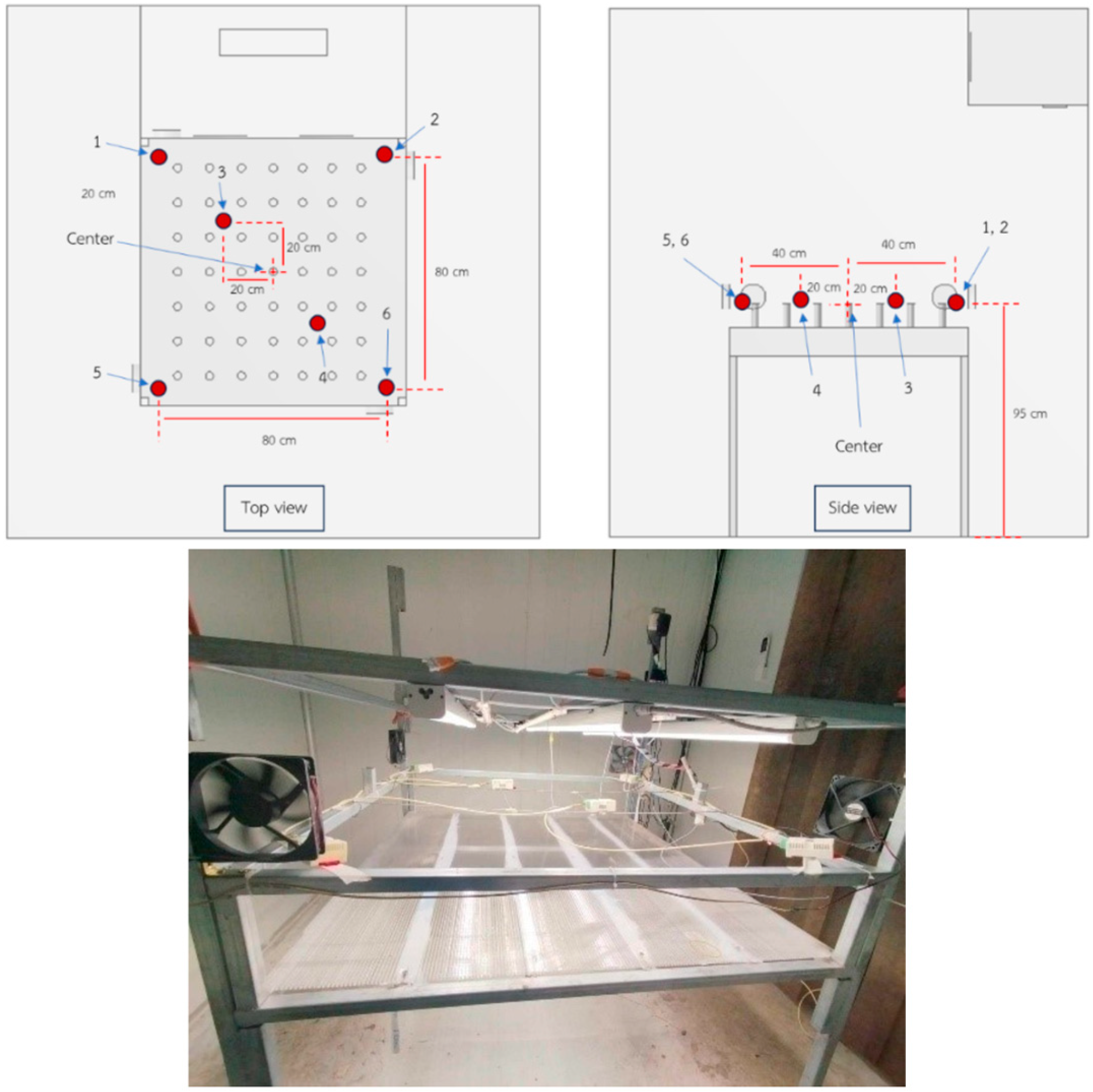
2.4. Verification of the Computational Fluid Dynamics Model

This research employs a systematic analytical approach to evaluate airflow patterns and temperature distribution within a controlled refrigeration chamber designed for optimal seedling growth conditions. The experimental setup incorporates six strategically positioned measurement points to monitor wind velocity and temperature variations throughout the chamber. These measurement locations have been carefully selected to provide comprehensive coverage of critical zones while ensuring balanced assessment of air circulation and temperature distribution patterns. Figure 3 presents a detailed schematic of the measurement point configuration, including precise distances between all six monitoring locations, facilitating accurate data collection and result validation.

The experimental design comprises ten distinct test scenarios, as illustrated in Figure 1 and Figure 2. The baseline configuration (Case 1) represents the control condition without fan installation within the refrigerated planting chamber (Figure 1). The subsequent nine configurations (Cases 2–10) incorporate a compact fan positioned at various locations within the cooling chamber to evaluate different ventilation strategies.

The measurement positions are systematically arranged in a grid pattern (L1, M1, R1, L2, M2, R2, L3, M3, and R3), as shown in Figure 2. Each position is specifically designated to analyze airflow patterns and corresponding temperature variations within the chamber. Data collection is conducted at a consistent elevation matching the plant height across all six monitoring points, ensuring accurate assessment of airflow dynamics and temperature distribution within the experimental environment.

2.5. Quality of the Grid

The mesh generation process employed ANSYS Meshing software v 19.1 with automatic tetrahedral mesh generation techniques to achieve mesh independence (Figure 4). Quality parameters including skewness, orthogonal quality, and aspect ratio were monitored throughout the meshing process to ensure computational accuracy. The mesh quality criteria were maintained within acceptable ranges: maximum skewness < 0.95, minimum orthogonal quality > 0.1, and aspect ratio < 100.

A systematic mesh independence study was conducted using a reference case with a room air temperature of 27 degrees Celsius. The analysis involved progressive refinement of mesh elements, starting from a coarse mesh and systematically reducing element size while monitoring the temperature at the upper central position as the primary response variable. The mesh refinement process was automated using size controls and growth rate parameters within ANSYS Meshing.

The results demonstrated mesh independence at approximately 1.26 × 10⁶ tetrahedral elements, where the temperature value at the central upper location stabilized.

2.6. Statistical Assessment

All the characteristics outlined significantly influence the temperature within the refrigerated room. Employing the Computational Fluid Dynamics (CFD) approach to analyze individual variances, the installation point is modified to facilitate the flow of dispersed air. Temperature averages were assessed using one-way ANOVA at a 95% confidence level, with the Least Significant Difference (LSD) method employed for comparative analysis of differences. Additionally, a correlation coefficient was calculated to elucidate the relationship among the various temperature types.

The R-squared (R²) coefficient of determination is calculated using the following formula:

R² = 1 − (SSres/SStot)

where SSres (Sum of Squares of Residuals) represents the sum of squared differences between predicted and actual values.

SSres = Σ(yi − ŷi)²

• yi is the observed value.
• ŷi is the predicted value from the model.

SStot (Total Sum of Squares) measures the total variation in the data:

SStot = Σ(yi − ȳ)²

• ȳ is the mean of observed values.

The Mean Absolute Percentage Error (MAPE) is calculated as:

MAPE = (100/n) × Σ|((Actual − Predicted)/Actual)|

The Nash–Sutcliffe Efficiency (NSE) is determined by:

NSE = 1 − [Σ(Oi − Pi)²/Σ(Oi − Ōi)²]

where

• Oi represents observed values.
• Pi represents predicted values.
• Ōi represents the mean of observed values.

Interpretation of NSE.

• NSE = 1 indicates perfect model performance.
• NSE > 0.8 indicates very good model performance.
• NSE < 0 indicates unsatisfactory model performance.

2.7. The Creation of the Computational Domain and Boundary Conditions

In creating the computational domain for the CFD model in this study, various parameters were considered, such as the size and shape of the experimental room which had dimensions of 2 m × 2 m × 2.2 m, the size and position of the plant-growing table which was 1 m × 1 m and 0.87 m high, as well as the size and position of the fans installed in the room (as shown in Figure 1).

Figure 1 shows the boundary conditions used in creating the CFD model for this study, which include the position and size of the room, plant-growing table, and fans.

2.8. CFD Model Validation

Verification of Computational Fluid Dynamics (CFD) models was conducted by utilizing data compiled from laboratory experiments to compare the results obtained from the cool room environment with those generated by simulations. To ensure the accuracy of the measured data in relation to the simulation outcomes, the root mean square error (RMSE) and average absolute error (AAE) were calculated as follows: [31].

$$\overline{V}={\displaystyle \frac{1}{m}}{\displaystyle \sum _{i=1}^m\left|x_{pi}-x_{mi}\right|}$$

(5)

$$RMSE=\sqrt{{\displaystyle \frac{{\displaystyle \sum _{m=1}^m{(x_{pi}-x_{mi})}^2}}{m}}}$$

(6)

where $m$ denotes the number of parameters, $x_{pi}$ represents the simulated data, and $x_{mi}$ signifies the measured data.

The present research investigation aims to examine the impact of various fan placements on air distribution within the experimental environment. A total of 10 cumulative attributes will be analyzed to assess the air circulation that influences environmental conditions within the structure, while excluding other variables such as drainage, photosynthesis, and vegetation layout.

The experiment is conducted by designating the fan installation site M1 as the primary location for the evaluation. To ensure adherence to established standards, it is imperative to verify the accuracy and reliability of the Computational Fluid Dynamics (CFD) model employed in the study. The SHT20 Temperature Humidity Sensor Module, managed by a microcontroller, possesses an accuracy of ±3% RH and ±0.5 °C.

3. Results

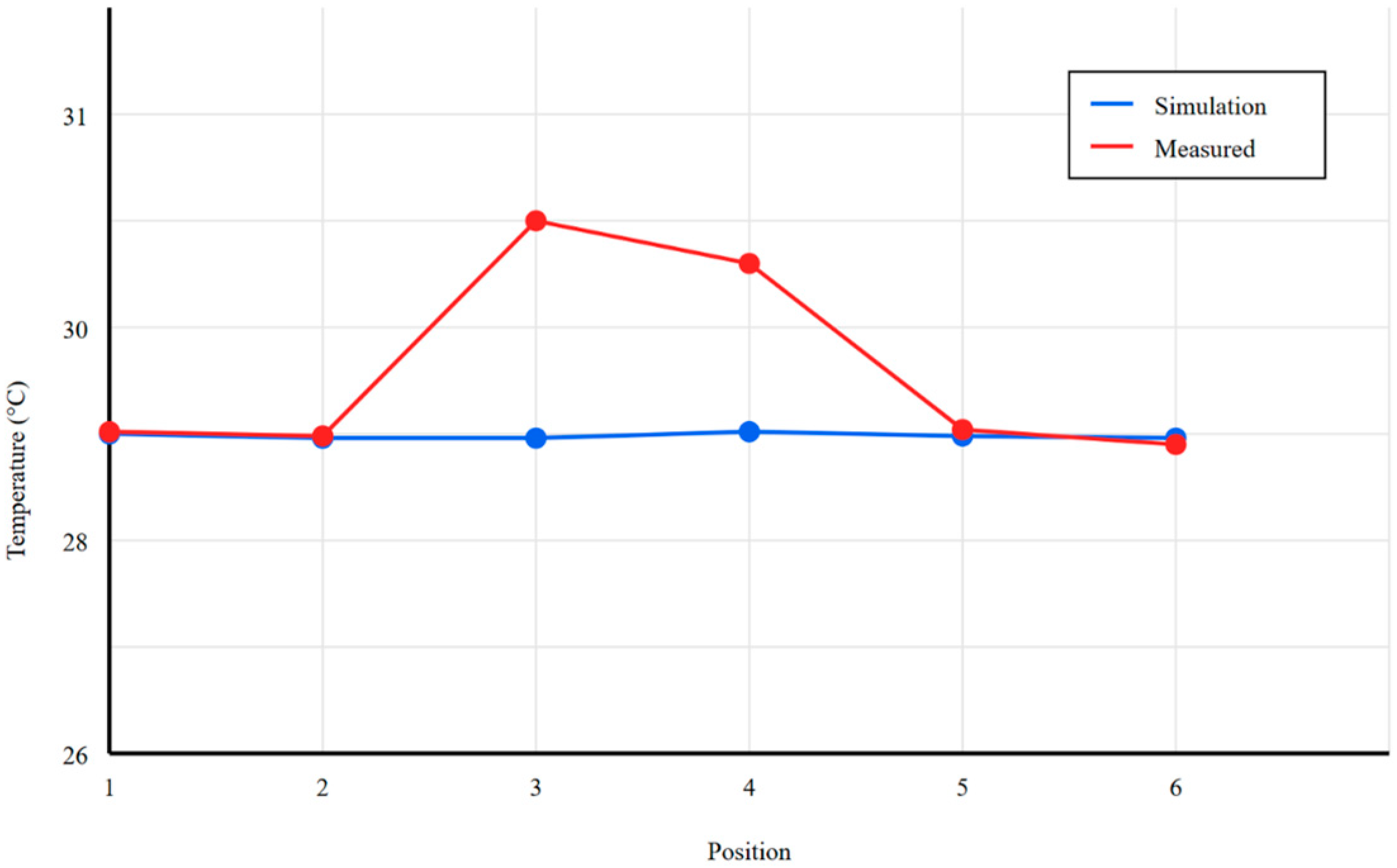
3.1. Results of CFD Model Validation

Data were recorded at 5-second intervals over 1 h, then averaged. The Root Mean Square Error (RMSE) was 2.02 °C for temperature and the Average Absolute Error (AAE) was 1.17 °C. These align with results reported in other studies [32]. However, the model’s predicted temperature and cooling values diverged from the 1.6 °C measurements recorded in the test room (Figure 5).

3.2. Results of the CFD Simulation on the Aerodynamic Environment

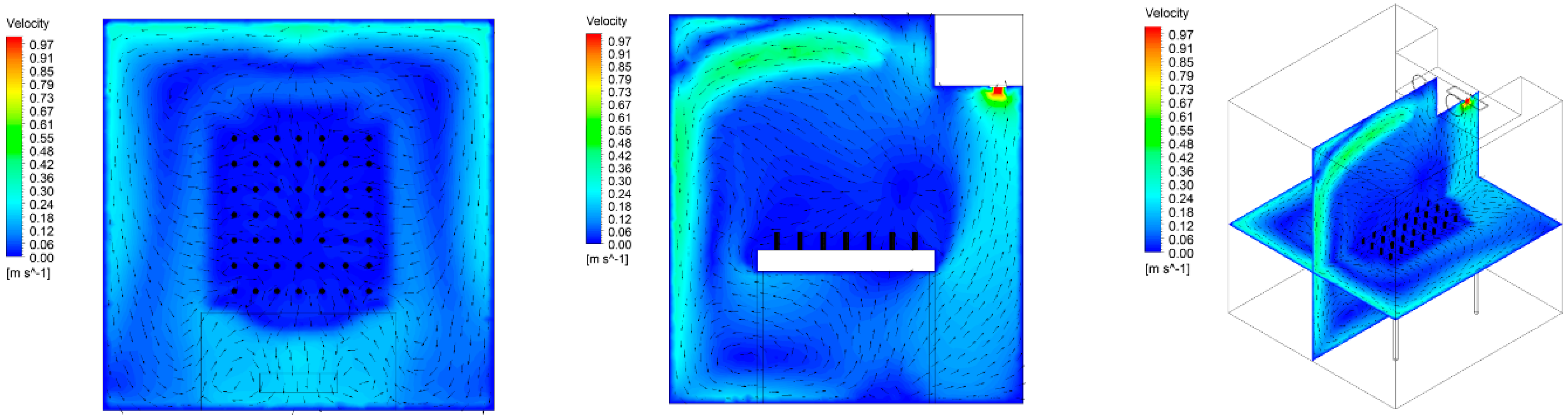
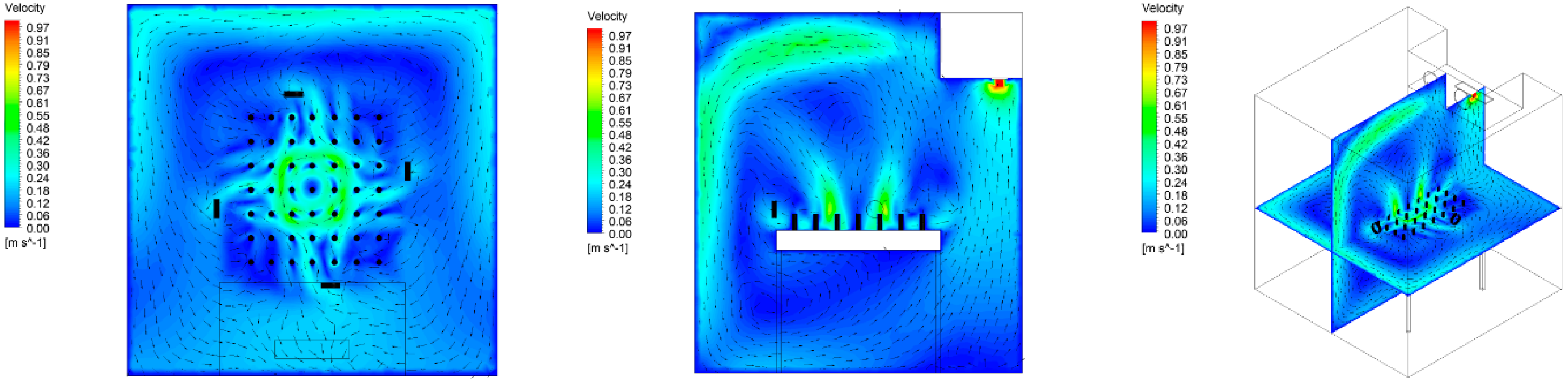
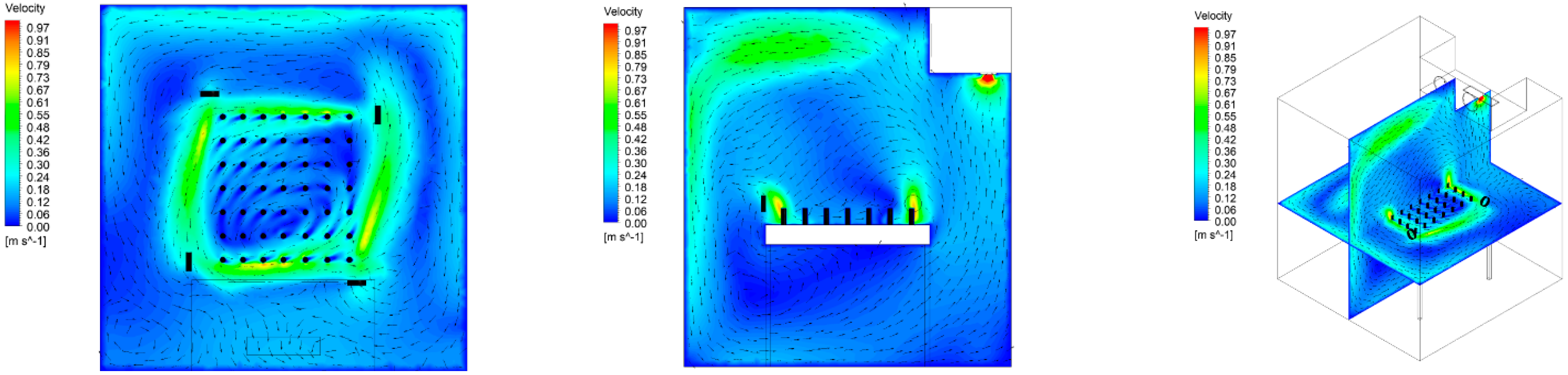
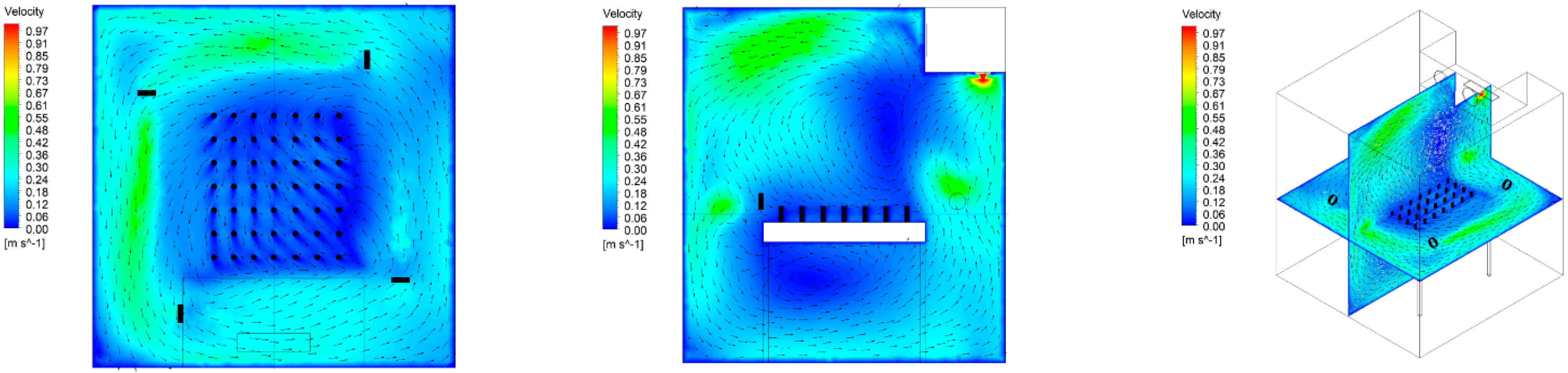
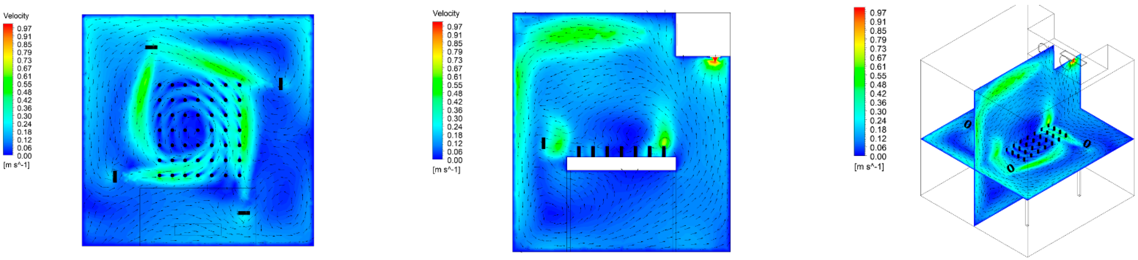
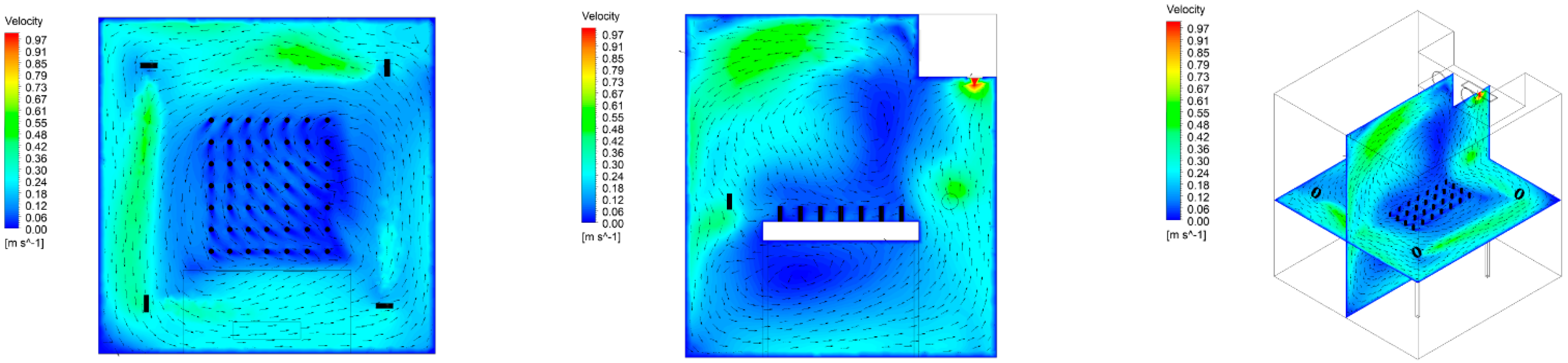
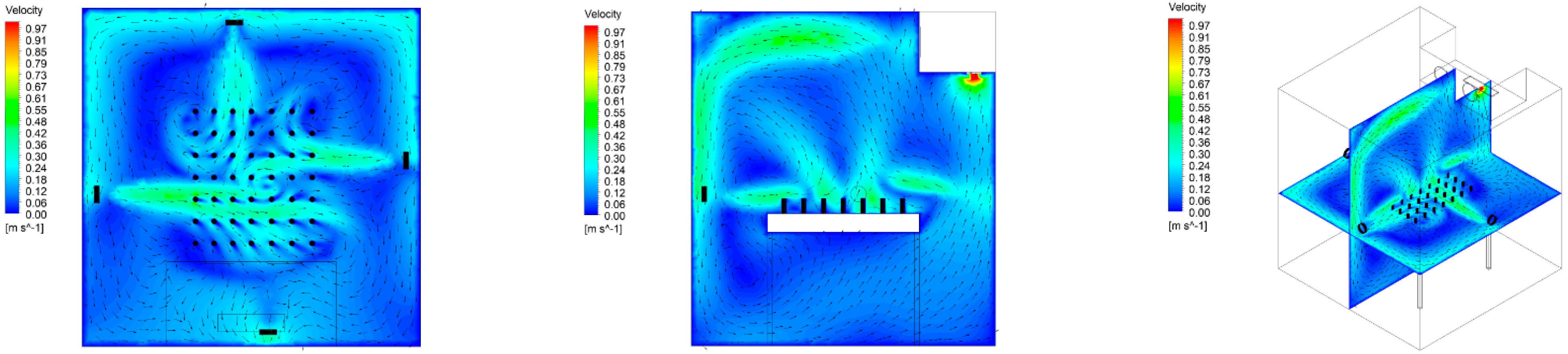
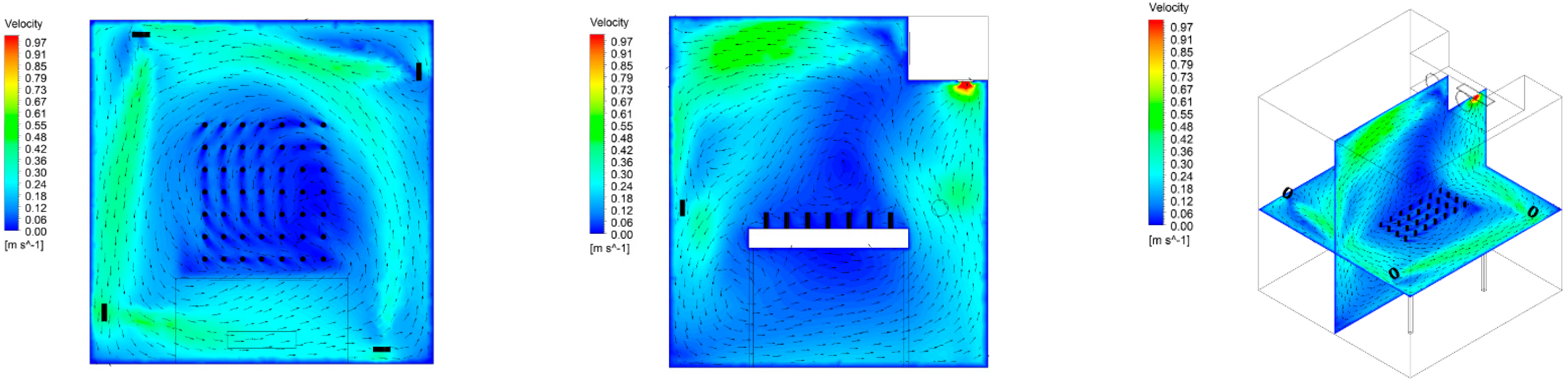
3.2.1. Results of the Wind Velocity Assessment in the Refrigeration Chamber

The findings of the Computational Fluid Dynamics (CFD) research provide a comprehensive analysis of airflow dynamics and fluctuations in wind speed. A one-way ANOVA was employed to evaluate the conditions and variations of factors influencing air dispersion within the refrigeration chamber. The results indicated that the placement of each fan, defined by the connection point of the ventilator, facilitated an analysis of the building’s variability, as illustrated in

Table 3. Comparison of air flow in the refrigerator (m/s).

Fan Installation Location	Multiple Comparisons
	NO Fan	L1	M1	R1	L2	M2	R2	L3	M3	R3
NO Fan	1	−0.11617	−0.29500 *	−0.04417	−0.11433	−0.23317 *	−0.05000	−0.09950	−0.14283 *	−0.05733
L1		1	−0.17883 *	0.07200	0.00183	−0.11700	0.06617	0.01667	−0.02667	0.05883
M1			1	0.05883 *	0.18067 *	0.06183	0.24500 *	0.19550 *	0.15217 *	0.23767 *
R1				1	−0.07017	−0.18900 *	−0.00583	−0.05533	−0.09867	−0.01317
L2					1	−0.11883	0.06433	0.01483	−0.02850	0.05700
M2						1	0.18317 *	0.13367 *	0.09033	0.17583 *
R2							1	−0.04950	−0.09283	−0.00733
L3								1	−0.04333	0.04217
M3									1	0.08550
R3										1
Mean (m/s)	0.0215	0.1377	0.3165	0.0657	0.1358	0.2547	0.0715	0.121	0.1643	0.0788
ANOVA		Sum of Squares	df	Mean Square	F	Sig.
Between Groups		0.439	9	0.049	4.287	0.000
Within Groups		0.569	50	0.011
Total		1.008	59

* The mean difference is significant at the 0.05 level.

. Notably, the study revealed that each wind speed exhibited statistically significant variations (p < 0.05) within a 95% confidence interval. These findings suggest that alterations in the environmental parameters surrounding the plants significantly influenced the rate of wind dispersion in the laboratory setting.

The rationale for selecting the installation site was to optimize the circulation of cold air within the cultivation area, allowing the plants to adapt to the natural airflow conditions. The air dispersion statistics confirmed that the fan arrangement effectively generated air circulation, with point M1 demonstrating the highest average airspeed relative to the other locations. This configuration had a considerable impact on the airflow rate when compared to all tested scenarios, with the exception of point M2, which was positioned at notably different installation distances. Additionally, the arrangement of measurement points varied, with M2 recording an average velocity of 0.2547 m/s and M3 recording an average velocity of 0.1643 m/s. The strategic placement of the fan along the edge of the vegetable planting table proved to enhance air circulation more effectively than other configurations.

Analysis of Variance (ANOVA) revealed statistically significant differences (p < 0.05) among the ten fan installation positions, with an F-value of 4.287 indicating clear distinctions between groups. The model’s accuracy assessment showed an R-squared value of 0.892, suggesting that the model could explain 89.2% of the data variance. However, considering only the R-squared value might not be sufficient for evaluating model accuracy, leading to additional analyses using MAPE and NSE metrics.

Comparison between simulation and experimental data demonstrated high correlation, particularly in low to moderate wind velocity ranges (0–0.2 m/s). However, discrepancies tended to increase at higher wind velocities (>0.3 m/s), most notably at position M1, which exhibited the highest wind speed. Trend analysis also revealed an inverse relationship between temperature and wind velocity, where areas with higher wind speeds showed lower temperatures (Figure 6).

Position M1 demonstrated optimal performance in both temperature reduction and air distribution, maintaining an average temperature of 27.03 °C and wind velocity of 0.317 m/s. Conversely, positions R1–R3 showed the lowest efficiency, indicating that excessive distance between fan installation and the growing table negatively impacts ventilation effectiveness. These trends align with airflow theory and previous research findings (Figure 7).

To evaluate model accuracy, this study employed two statistical parameters: Mean Absolute Percentage Error (MAPE) and Nash–Sutcliffe Efficiency (NSE). The analysis revealed a MAPE value of 0.643%, which being below 10% indicates high model accuracy. The NSE value of 0.886 exceeded 0.8, demonstrating excellent model performance. Generally, NSE values range from −∞ to 1, where 1 represents perfect model performance, and values below 0 indicate unsuitable model performance.

These statistical metrics confirm that the developed CFD model exhibits high accuracy and reliability, making it effective for predicting airflow behavior and temperature distribution in cold storage systems for medicinal plant cultivation.

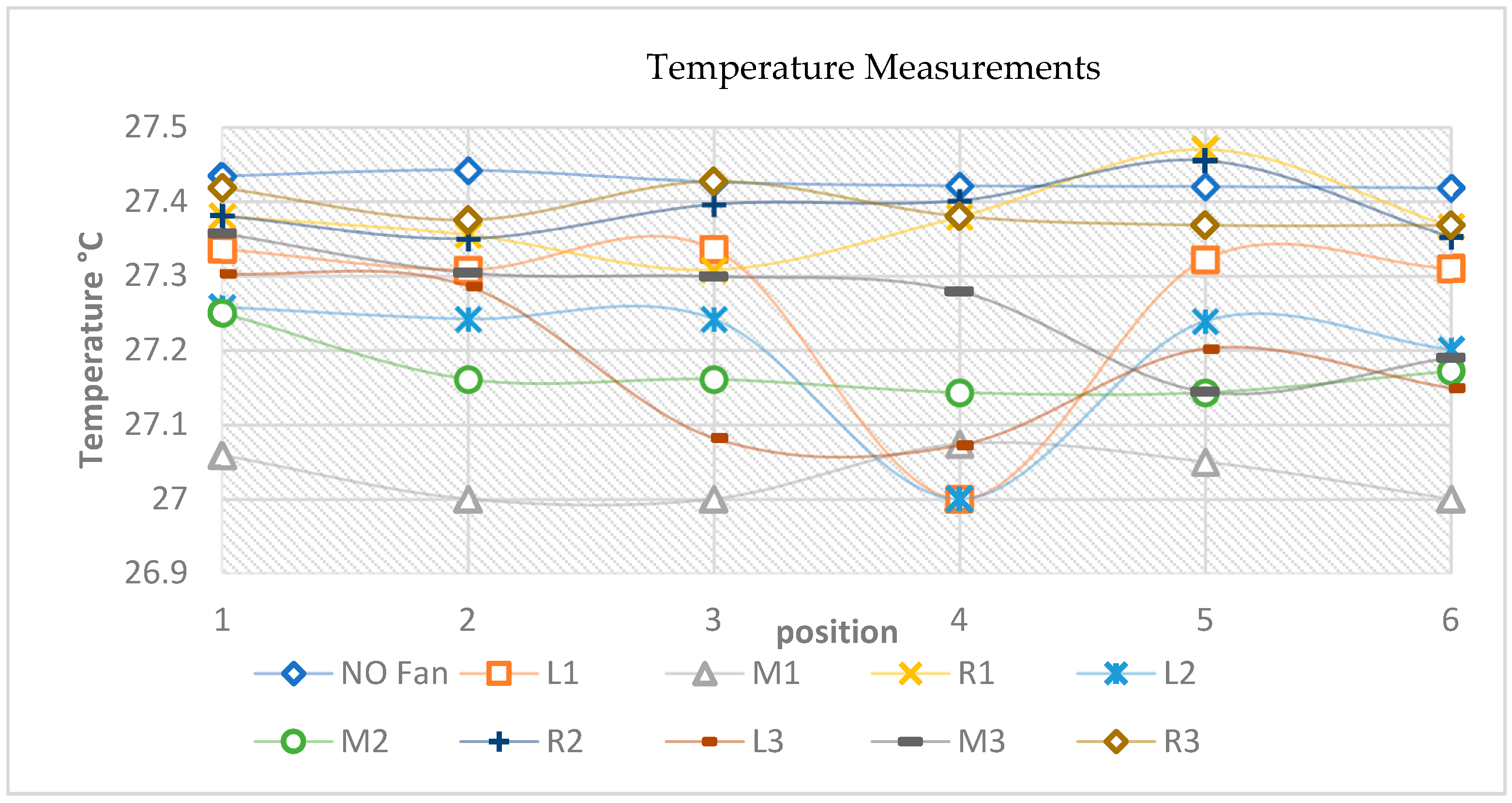
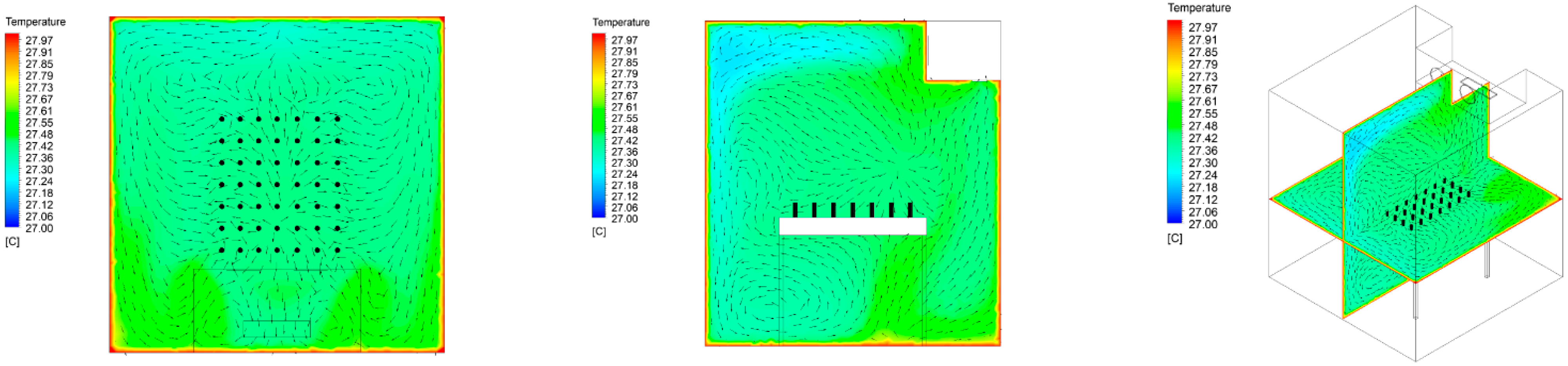
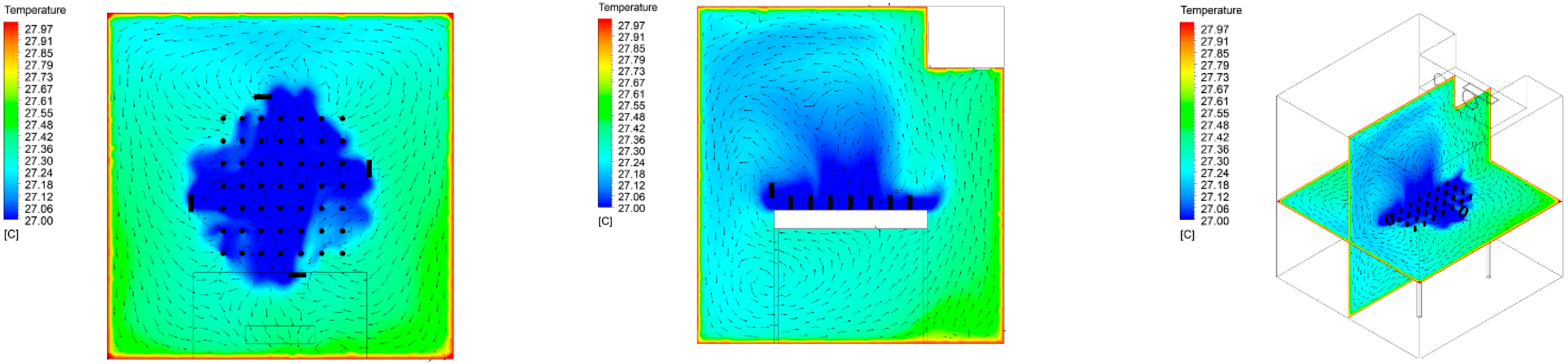
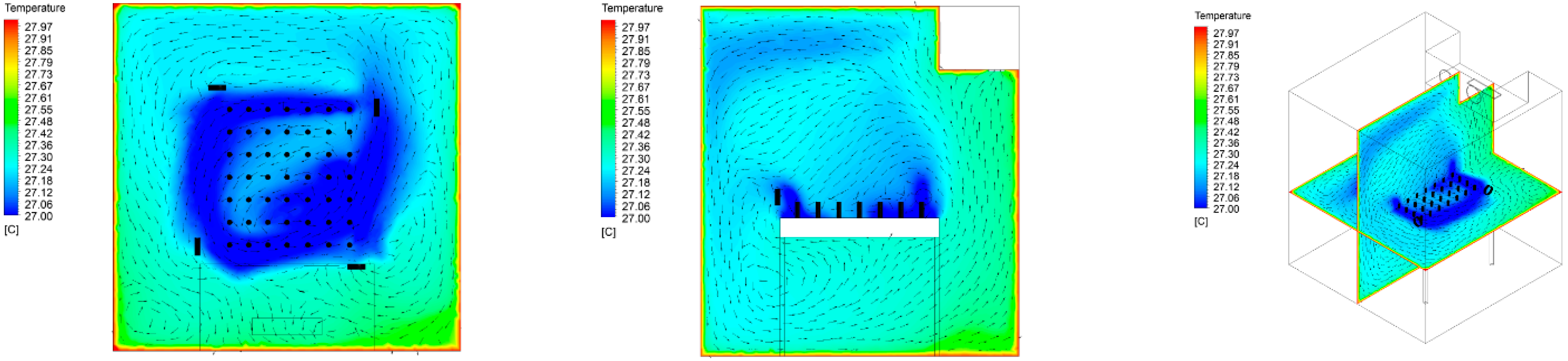
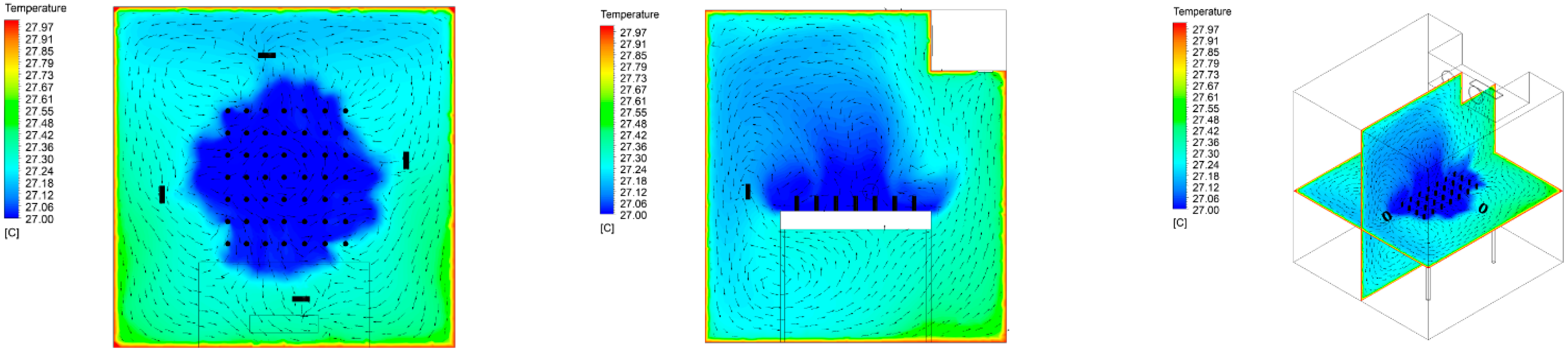
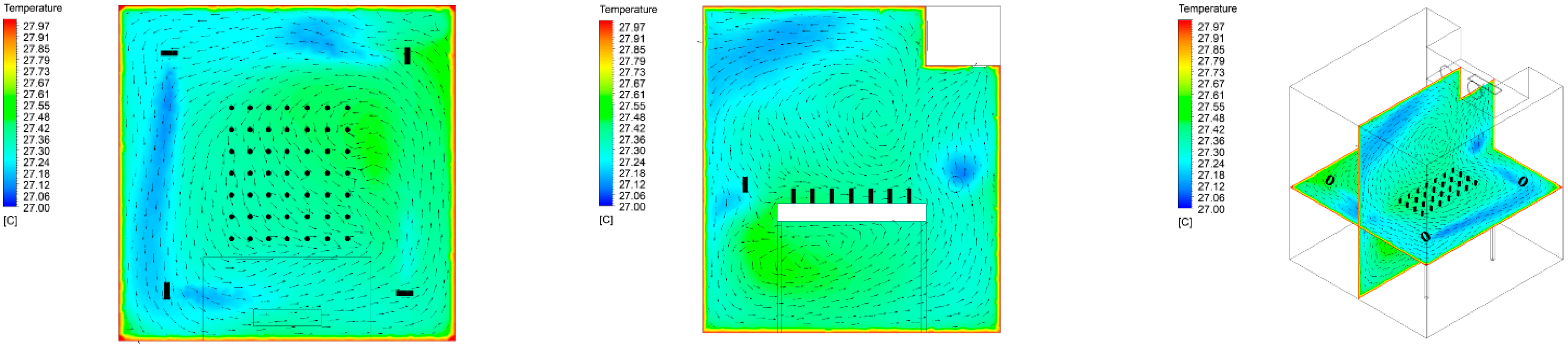
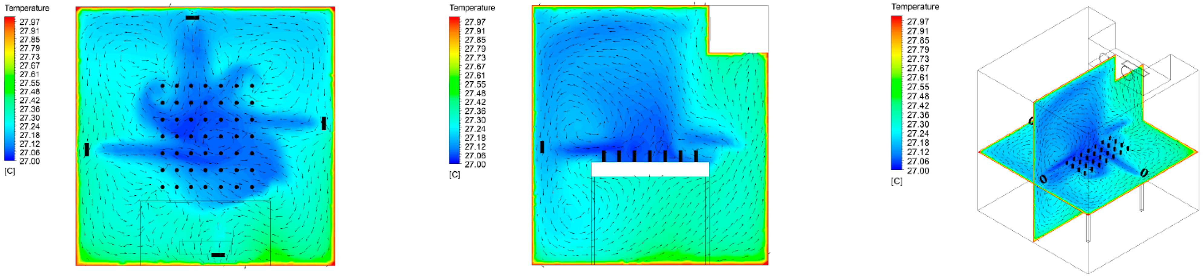
3.2.2. Results of Air Temperature Measurements in the Refrigerator

This analytical assessment investigates the variations in airflow under different operational conditions. The findings provide a comparative analysis of airflow in scenarios where the fan is immobilized versus those characterized by varying wind conditions. Employing the one-way ANOVA statistical method, this study systematically evaluates and compares the characteristics of airflow and wind speed variations across a spectrum of conditions, each influenced by multiple factors impacting air distribution performance within the refrigeration unit. The precise location of the ventilator emerges as a critical variable in this evaluation. Each distinct installation of the ventilator produces results demonstrating statistically significant variance (p < 0.05) at a 95% confidence level. Notably, the installation of the fan at point M1 yields significant temperature variations relative to the fan’s installation point, with each measurement point exhibiting statistical significance, thereby designating M1 as the most effective location for optimizing airflow regulation.

In contrast, the fan installation at point R, associated with the evaluation of air circulation, exhibits the highest temperature range compared to other locations. The average temperature at this point fluctuates between 27.37 °C and 27.39 °C, rendering it unsuitable for effective air dispersion and suggesting inadequate operational efficiency.

The model conducted a comprehensive analysis of temperature readings obtained from all six measurement sites and subsequently presented the findings. As illustrated in

Table 4. Comparison of Indoor Air Temperature (°C).

Fan Installation Location	Multiple Comparisons
	NO Fan	L1	M1	R1	L2	M2	R2	L3	M3	R3
NO Fan	1	0.15817 *	0.39633 *	0.05050	0.22983 *	0.25517	0.03767	0.24450 *	0.16467 *	0.03750
L1		1	0.23817 *	−0.10767 *	0.07167	0.09700 *	−0.12050 *	0.08633 *	0.00650	−0.12067 *
M1			1	−0.34583 *	−0.16650 *	−0.14117 *	−0.35867 *	−0.15183 *	−0.23167 *	−0.35883 *
R1				1	0.17933 *	0.20467 *	−0.01283	0.19400 *	0.11417 *	−0.01300
L2					1	0.02533	−0.19217 *	0.01467	−0.06517	−0.19233 *
M2						1	−0.21750 *	−0.01067	−0.09050 *	−0.21767 *
R2							1	0.20683 *	0.12700 *	−0.00017
L3								1	−0.07983	−0.20700 *
M3									1	−0.12717 *
R3										1
Mean (°C)	27.4268	27.2687	270.0305	27.3763	27.1970	27.1717	27.3892	27.1823	27.2622	27.3893
ANOVA		Sum of Squares	df	Mean Square	F	Sig.
Between Groups		0.867	9	0.096	18.837	0.000
Within Groups		0.256	50	0.005
Total		1.122	59

* The mean difference is significant at the 0.05 level.

and Figure 8, the installation of a small fan to enhance air movement and ventilation significantly contributed to the reduction of temperature within the ventilated space. The average temperature recorded across the six sites revealed that location M1 exhibited the lowest temperature of 27.03 °C, indicating that the fan placement at this point was the most effective in promoting cooler temperatures and improved air circulation.

The superior performance of the M1 fan location can be attributed to its strategic placement at the corner of the plant-growing table. This position allows the fan to direct airflow along the edges of the table, creating a circular motion that efficiently distributes cool air to all corners. As a result, the temperature remains consistent throughout the growing area, providing optimal conditions for plant development. In contrast, other fan locations, such as L1 and R1, may create uneven airflow patterns, leading to temperature gradients that can negatively impact plant growth.

Temperature plays a crucial role in plant development, as it directly influences various physiological processes such as photosynthesis, respiration, and transpiration. Excessively high temperatures can lead to heat stress, causing damage to plant tissues and inhibiting growth. On the other hand, cooler temperatures within the optimal range promote healthy plant development by facilitating efficient nutrient uptake, water transport, and enzymatic activities. Therefore, maintaining a consistent and suitable temperature, as achieved by the M1 fan location, is essential for creating an ideal environment for plant growth.

The analysis also revealed that the fan placement at point R, particularly R1, R2, and R3, exhibited the worst performance in terms of temperature and air circulation. These locations, being the farthest from the plant-growing table, failed to effectively direct airflow towards the plants. Instead, the airflow remained concentrated along the periphery of the table, resulting in higher average temperatures ranging from 27.35 °C to 27.42 °C. The lack of direct airflow over the plants led to reduced cooling efficiency and suboptimal growing conditions.

To improve the performance of the R fan locations, several modifications could be considered. Firstly, adjusting the fan orientation or using multiple fans to create a more targeted airflow towards the plant-growing area could help enhance cooling effectiveness. Additionally, implementing air guides or baffles to redirect the airflow from the periphery towards the center of the table could promote better air circulation. Furthermore, increasing the fan speed or using fans with higher airflow capacities could compensate for the increased distance between the fan and the growing area, ensuring adequate air movement and temperature regulation.

This section delineates the three-dimensional air circulation patterns, illustrating the dispersion of air that acts as a carrier for carbon dioxide (CO₂), a critical component for enhancing plant metabolic output. This process facilitates the synthesis of essential biomolecules in conjunction with adequate illumination. The graphical representation further depicts the arrangement of equipment and the elevation of the planting area, which is established by a total of six wind speed measurement stations.

In the absence of a fan (Figure 9), air circulation is entirely dependent on the airflow from the supply air, which generates a circulating breeze determined by the orientation of the air ducts delivering cold air. This airflow descends from the upper region opposite the air conditioner, resulting in suboptimal air circulation above the plant-growing table, with average air velocities ranging from 0.011 to 0.035 m/s.

When a small fan is positioned at point L1 (Figure 10), it significantly enhances air circulation in accordance with the fan’s orientation, effectively drawing ambient air into the center of the plant-growing table. Consequently, wind speeds at this location reach levels of 0.376 m/s, with an average speed of 0.138 m/s recorded across all six measurement sites.

The installation of the fan at point M1 (Figure 11), located at the corner of the plant-growing table, is characterized by a circulation pattern that initiates airflow around the table in response to the fan’s wind direction. This configuration effectively distributes air to each corner, resulting in circular airflow around the table, with maximum velocities recorded along its circumference ranging from 0.394 to 0.511 m/s, and an average peak speed of 0.317 m/s.

In contrast, the installation of the fan at point R1 (Figure 12) positions the fan at a considerable distance from the plant-growing table, leading to air circulation that predominantly occurs around the table’s periphery. As a result, the designated planting area suffers from inadequate air circulation, exhibiting an average velocity of only 0.066 m/s.

The L2 fan block configuration (Figure 13) enhances airflow circulation near the planting table through lateral ventilation, facilitated by the suction force of a compact fan. This setup maintains optimal indoor air quality within the test chamber, achieving an average velocity of 0.136 m/s. Notably, significantly higher velocities are observed at the table’s center compared to its peripheral areas.

In the M2 layout (Figure 14), fan blocks positioned at the table corners generate pressure gradients that distribute airflow throughout the planted area. This arrangement creates circular air patterns, particularly pronounced along the table edges, resulting in an average velocity of 0.255 m/s.

The R2 configuration (Figure 15), which features a fan mounted at a considerable distance from the planting table, results in airflow primarily concentrated around the table’s exterior. Consequently, the planting locations experience minimal air movement, with an average velocity of only 0.072 m/s.

The inadequate air circulation at point R1 can be attributed to three primary factors.

(1)

The substantial distance between the fan and planting table.

(2)

Fan orientation that directs airflow toward peripheral areas rather than the central zone.

(3)

Physical obstruction created by the table structure.

To enhance air circulation, several potential solutions should be considered:

(1)

Repositioning the fan in closer proximity to the table.

(2)

Modifying the fan’s orientation to direct airflow toward the central area.

(3)

Installing air guidance systems.

(4)

Implementing a multiple-fan configuration.

In the L3 ventilator configuration (Figure 16), despite being positioned at a considerable distance from the planting table, the airflow is effectively directed toward the table’s central region. This setup maintains a consistent mean velocity of 0.121 m/s with minimal fluctuations.

The M3 installation point (Figure 17) demonstrates limited airflow penetration into the planting table area. Due to its significant distance from the external environment, air conduction toward the center is negligible.

In the R3 configuration (Figure 18), while the overall airflow exhibits an average velocity of 0.164 m/s, the impact on the planting area remains minimal. Although external air movement is present, the planting zone experiences limited air circulation, with a mean velocity of only 0.079 m/s.

Air dispersion patterns significantly influence temperature distribution, with effective circulation playing a crucial role in temperature reduction. Optimized air management facilitates the provision of essential growth factors by maintaining an ideal temperature of 27 °C, thereby enhancing plant growth efficiency. The simulation results are presented through three-dimensional visualizations, based on temperature measurements from six distinct points.

In the control setup without fan-assisted circulation (Figure 19), the table area maintains relatively stable temperatures. The plant zone, primarily cooled by ambient air, records temperatures between 27.41 °C and 27.43 °C. The L1 configuration (Figure 20) demonstrates that even with an inactive fan, the induced airflow contributes to temperature reduction along its path. This cooling effect influences the planting table vicinity, resulting in an average temperature of 27.27 °C.

The M1 configuration (Figure 21) exhibits temperature distribution patterns influenced by the ventilation system’s airflow characteristics, maintaining an average temperature of 27.03 °C. In contrast, the R1 configuration (Figure 22) shows limited air dispersion, with wind currents directed away from the planting table, resulting in temperatures ranging from 27.35 °C to 27.47 °C.

The L2 small fan installation point (Figure 23) effectively demonstrates temperature distribution patterns, with notable air circulation around the planting table. The areas experiencing airflow show reduced temperatures, maintaining an average of 27.20 °C.

In the M2 configuration (Figure 24), air distribution across the table exhibits uniform dispersion patterns, though the impact of airflow remains moderate. Air circulation primarily concentrates in the central area, resulting in an average temperature of 27.17 °C.

The R2 configuration (Figure 25), with its installation point positioned at a considerable distance from the table edge, generates greater peripheral air circulation compared to cooling air distribution at the planting table area. This arrangement maintains an average temperature of 27.39 °C.

For the final three configurations, the L3 fan installation (Figure 26) demonstrates airflow patterns guided by fan-induced forces. The air movement follows a distinctive pattern, flowing toward the center of the planting table before curving and circulating outward along the peripheral areas. This configuration maintains an average temperature of 27.18 °C.

The M3 configuration (Figure 27) shows minimal temperature impact on the planting table area. Due to the peripheral positioning of installation points, temperature dispersion primarily occurs around the outer regions, resulting in an average temperature of 27.26 °C.

In the R3 configuration (Figure 28), the installation distance prevents effective cooling air delivery to the planting table area. Consequently, temperatures around the planting table range between 27.36 °C and 27.42 °C.

This study found a temperature difference of approximately 0.36 °C between the optimal case (M1: 27.03 °C) and the least effective positions (R positions ~27.39 °C), which was statistically significant (p < 0.05). However, from a practical perspective, most plants can tolerate this temperature range, suggesting limited biological significance. The primary advantage of the M1 fan position lies in creating a more uniform environment through improved air circulation (0.317 m/s), consistent temperature distribution, and enhanced CO₂ dispersal for photosynthesis. These conditions may promote more uniform plant growth, reduce disease risks associated with stagnant air, and improve pollination efficiency in flowering plants.

From an investment and energy perspective, while small fans are relatively inexpensive and consume less energy compared to HVAC systems, they still incur installation and maintenance costs. The 0.36 °C temperature improvement may not justify the investment in all scenarios. The actual impact on yield requires further research, and the cost–benefit ratio varies depending on factors such as medicinal plant species, market value, local energy costs, and climatic conditions. Implementation should be considered primarily for high-value medicinal plant production requiring precise environmental control. Decision-making should be based on case-specific cost-benefit analyses considering these variables rather than temperature differences alone.

4. Discussion

Research in Computational Fluid Dynamics (CFD) underscores the critical importance of ventilation design, particularly the deliberate configuration of input channels. The incorporation of a fan has been shown to enhance airflow efficiency and reduce cooling energy demands by facilitating improved air circulation [33]. Although the installation of an insect-proof screen provides advantages for pest control, it may hinder ventilation; nonetheless, the strategic use of a fan can alleviate this issue by promoting adequate airflow and minimizing the vibrational effects induced by the screen [34].

Integrating a fan within an evaporative cooling system effectively controls humidity and temperature, especially in humid conditions. Additionally, using air retention strategies in a greenhouse with an Earth-to-Air Heat Exchanger (EAHE) enhances thermal efficiency by promoting uniform air distribution, which is crucial for optimizing heat exchange rates and maintaining stable climatic conditions [35].

Furthermore, studies investigating the spatial variation of air temperature and vapor pressure deficit (VPD) in greenhouses outfitted with organic solar cell modules (OPVs) suggest that fans can play a significant role in regulating these parameters by enhancing the uniformity of air distribution. Consequently, the judicious deployment of fans is essential in multi-scale glasshouses to foster plant growth under diverse shading conditions [36]. This consideration is particularly pertinent, as airflow patterns may become intricate due to factors such as structural design, plant interactions, and insect filtration. Consistent air circulation facilitated by fans mitigates heat emissions that could detrimentally impact crop quality and yield [37].

Additionally, in experimental glasshouse designs, such as octagonal structures, the utilization of fans significantly contributes to natural air cooling by increasing air velocity and enhancing temperature distribution, thereby playing a vital role in the environmental sustainability of crop growth [38]. The fan is essential for regulating the thermal environment in a greenhouse. Ventilated evaporative cooling systems enhance air circulation and cooling efficiency, making them popular for managing temperature and humidity. This system cools air by passing it through a wetted plate, using evaporation before distributing it throughout the greenhouse, leading to significant temperature reductions. Research indicates that this fan system can lower air temperature by 20.6 °C, with ground temperatures at 13.0 °C and cover temperatures at 20.6 °C, functioning at an airspeed of 4.4 m/s with a sheet thickness of 6 cm [39].

Moreover, the application of grounded fans in experimental greenhouses has resulted in decreased energy consumption while maintaining optimal conditions for plant growth. An independent study reported temperature ranges between 16 °C and 26 °C, accompanied by a relative humidity level of 65% [40]. The operation of a ventilation chamber, classified as a passive fan system, has been shown to significantly enhance airflow patterns, resulting in a more uniform temperature distribution, with a temperature differential from the external environment not exceeding 1.1 °C [41]. Additionally, a distributed ventilation system has been proposed in conjunction with bio-humidifier cooling to sustain ideal conditions for banana cultivation, maintaining temperatures between 21 °C and 26 °C and relative humidity levels between 50% and 70% [42].

In the context of hybrid systems, the performance of fans is evaluated alongside air-to-water heat pumps, solar panels, and coil fan assemblies to fulfill greenhouse cooling requirements. While the capacity of coil fans may require augmentation during peak summer temperatures [43], the deployment of active ventilation solutions within integrated greenhouses may yield energy efficiencies that are double those of passive systems. This underscores the vital role of fans in enhancing energy efficiency, reducing consumption, and promoting sustainability [44]. Furthermore, predictive models for semi-closed greenhouses indicate that fans are pivotal in regulating cooling and water requirements. Recent advancements in computational methodologies, particularly the application of Long Short-Term Memory (LSTM) models, have been employed to delineate these criteria with greater precision [45].

The establishment of herb cultivation rooms for the future is underscored by the application of computational fluid dynamics (CFD), a critical tool for modeling the complex interactions inherent in growth conditions, including airflow, temperature, humidity, and CO2 concentrations [46]. The utilization of CFD not only reduces energy demands for computational analyses but also maintains a high level of accuracy in predicting pressure differentials and convective heat transfer [47]. Furthermore, advancements in air circulation systems may mitigate temperature variations between the upper and lower zones of the cultivation room, thereby enhancing conditions conducive to plant growth and reducing associated energy costs [48].

5. Conclusions

This research conducted a rigorous analysis of ventilator installation designs for air distribution using computational fluid dynamics (CFD) across ten distinct cases. The study compared a control case without ventilation (Case 1) against nine cases with strategically placed ventilators (Cases 2–10), evaluating their effects on airflow regulation through wind velocity and temperature measurements. Data was collected from six measurement points to assess the impact of fan installation on air mixing and circulation patterns.

The results demonstrated that position M1 achieved optimal performance with the highest wind speed of 0.173 m/s, while positions M2 and M3 recorded average wind speeds of 0.255 m/s and 0.164 m/s, respectively. Temperature analysis revealed M1 maintained the lowest average temperature of 27.03 °C, compared to 27.17 °C and 27.18 °C in other configurations. Statistical analysis confirmed significant differences in both wind speed and temperature measurements across different installation points.

These findings have several practical implications for plant cultivation, as follows:

(1)

Enhanced air circulation may improve photosynthetic rates through better CO₂ distribution.

(2)

More uniform temperature distribution could reduce heat stress on plants.

(3)

Improved ventilation may help prevent fungal diseases by reducing humidity pockets.

(4)

Better air mixing could contribute to stronger stem development through mechanical stimulation.

Practical recommendations for implementation include the following:

(1)

Positioning fans at optimal M1 locations in similar greenhouse layouts.

(2)

Considering multiple fan installations for larger cultivation areas.

(3)

Adjusting fan speeds based on specific crop requirements.

(4)

Regular monitoring of airflow patterns and temperature distribution.

Study limitations and future research directions.

(1)

Results are specific to the tested room configuration and size.

(2)

Further validation needed under varying environmental conditions.

(3)

Long-term effects on plant growth and development require investigation.

(4)

Cost–benefit analysis of different ventilation strategies recommended.

(5)

Impact on different plant species should be evaluated.

References

1. Zhang, Y.; Kacira, M. Analysis of climate uniformity in indoor plant factory system with computational fluid dynamics (CFD). Biosyst. Eng. 2022, 220, 73–86. [Google Scholar] [CrossRef]
2. He, R.; Ju, J.; Liu, K.; Song, J.; Zhang, S.; Zhang, M.; Hu, Y.; Liu, X.; Li, Y.; Liu, H. Technology of plant factory for vegetable crop speed breeding. Front. Plant Sci. 2024, 15, 1414860. [Google Scholar] [CrossRef] [PubMed]
3. Shang, Y.; Hasan, M.K.; Ahammed, G.J.; Li, M.; Yin, H.; Zhou, J. Applications of Nanotechnology in Plant Growth and Crop Protection: A Review. Molecules 2019, 24, 2558. [Google Scholar] [CrossRef] [PubMed]
4. Li, H.; Guo, Y.; Zhao, H.; Wang, Y.; Chow, D. Towards automated greenhouse: A state of the art review on greenhouse monitoring methods and technologies based on internet of things. Comput. Electron. Agric. 2021, 191, 106558. [Google Scholar] [CrossRef]
5. Si, C.; Qi, F.; Ding, X.; He, F.; Gao, Z.; Feng, Q.; Zheng, L. CFD Analysis of Solar Greenhouse Thermal and Humidity Environment Considering Soil–Crop–Back Wall Interactions. Energies 2023, 16, 2305. [Google Scholar] [CrossRef]
6. Li, K.; Mi, Y.; Zheng, W. An Optimal Control Method for Greenhouse Climate Management Considering Crop Growth’s Spatial Distribution and Energy Consumption. Energies 2023, 16, 3925. [Google Scholar] [CrossRef]
7. Zhang, W.; Zhang, W.; Yang, Y.; Hu, G.; Ge, D.; Liu, H.; Cao, H. A cloud computing-based approach using the visible near-infrared spectrum to classify greenhouse tomato plants under water stress. Comput. Electron. Agric. 2021, 181, 105966. [Google Scholar]
8. Farooq, M.S.; Javid, R.; Riaz, S.; Atal, Z. IoT based smart greenhouse framework and control strategies for sustainable agriculture. IEEE Access 2022, 10, 99394–99420. [Google Scholar] [CrossRef]
9. Contreras-Castillo, J.; Guerrero-Ibañez, J.A.; Santana-Mancilla, P.C.; Anido-Rifón, L. SAgric-IoT: An IoT-based platform and deep learning for greenhouse monitoring. Appl. Sci. 2023, 13, 1961. [Google Scholar] [CrossRef]
10. Liu, R.; Li, M.; Guzmán, J.L.; Rodríguez, F. A fast and practical one-dimensional transient model for greenhouse temperature and humidity. Comput. Electron. Agric. 2021, 186, 106186. [Google Scholar] [CrossRef]
11. Noh, K.; Jeong, B.R. Optimizing temperature and photoperiod in a home cultivation system to program normal, delayed, and hastened growth and development modes for leafy Oak-leaf and Romaine lettuces. Sustainability 2021, 13, 10879. [Google Scholar] [CrossRef]
12. Dutta, D.; Sharma, V.; Guria, S.; Chakraborty, S.; Sarveswaran, S.; Harshavardhan, D.; Roy, P.; Nandi, S.; Thakur, A.; Kumar, S.; et al. Optimizing plant growth and crop productivity through hydroponics technique for sustainable agriculture: A review. Int. J. Environ. Clim. Change 2023, 13, 933–940. [Google Scholar] [CrossRef]
13. Ma, X.K.; Liu, Y. Supramolecular purely organic room-temperature phosphorescence. Acc. Chem. Res. 2021, 54, 3403–3414. [Google Scholar] [CrossRef]
14. Yan, X.; Peng, H.; Xiang, Y.; Wang, J.; Yu, L.; Tao, Y.; Chen, R. Recent advances on host–guest material systems toward organic room temperature phosphorescence. Small 2022, 18, 2104073. [Google Scholar] [CrossRef]
15. Chen, M.T.; Zhang, R.L.; Feng, J.J.; Mei, L.P.; Jiao, Y.; Zhang, L.; Wang, A.J. A facile one-pot room-temperature growth of self-supported ultrathin rhodium-iridium nanosheets as high-efficiency electrocatalysts for hydrogen evolution reaction. J. Colloid Interface Sci. 2022, 606, 1707–1714. [Google Scholar] [CrossRef]
16. Zhang, S.; Zhuo, Y.; Ezugwu, C.I.; Wang, C.C.; Li, C.; Liu, S. Synergetic molecular oxygen activation and catalytic oxidation of formaldehyde over defective MIL-88B (Fe) nanorods at room temperature. Environ. Sci. Technol. 2021, 55, 8341–8350. [Google Scholar] [CrossRef]
17. Jagadish, S.K.; Way, D.A.; Sharkey, T.D. Plant heat stress: Concepts directing future research. Plant Cell Environ. 2021, 44, 1992–2005. [Google Scholar] [CrossRef] [PubMed]
18. Rajiv; Kumari, M. Protected Cultivation of High-Value Vegetable Crops Under Changing Climate. In Advances in Research on Vegetable Production Under a Changing Climate; Springer International Publishing: Cham, Switzerland, 2023; Volume 2, pp. 229–266. [Google Scholar]
19. Chimankare, R.V.; Das, S.; Kaur, K.; Magare, D. A review study on the design and control of optimised greenhouse environments. J. Trop. Ecol. 2023, 39, e26. [Google Scholar] [CrossRef]
20. Kumar, S.; Bairwa, D.S.; Kumar, K.; Yadav, R.K.; Yadav, L.P. Climate regulation in protected structures: A review. J. Agric. Ecol. 2022, 13, 20–34. [Google Scholar] [CrossRef]
21. Galieni, A.; D′Ascenzo, N.; Stagnari, F.; Pagnani, G.; Xie, Q.; Pisante, M. Past and future of plant stress detection: An overview from remote sensing to positron emission tomography. Front. Plant Sci. 2021, 11, 609155. [Google Scholar] [CrossRef]
22. Kaur, R.; Kumar, S.; Ali, S.A.; Kumar, S.; Ezing, U.M.; Bana, R.; Meena, S.; Dass, A.; Singh, T. Impacts of climate change on crop-weed dynamics: Challenges and strategies for weed management in a changing climate. Open J. Environ. Biol. 2024, 9, 015–021. [Google Scholar]
23. Kolupaev, Y.E.; Blume, Y.B. Plant Adaptation to Changing Environment and its Enhancement. Open Agric. J. 2022, 16, e187433152208251. [Google Scholar] [CrossRef]
24. de Wit, H.A.; Stoddard, J.L.; Monteith, D.T.; Sample, J.E.; Austnes, K.; Couture, S.; Evans, C.D. Cleaner air reveals growing influence of climate on dissolved organic carbon trends in northern headwaters. Environ. Res. Lett. 2021, 16, 104009. [Google Scholar] [CrossRef] [PubMed]
25. Yang, X.; Baskin, C.C.; Baskin, J.M.; Pakeman, R.J.; Huang, Z.; Gao, R.; Cornelissen, J.H. Global patterns of potential future plant diversity hidden in soil seed banks. Nat. Commun. 2021, 12, 7023. [Google Scholar] [CrossRef]
26. Norton, T.; Sun, D. Computational fluid dynamics (CFD)—An effective and efficient design and analysis tool for the food industry: A review. Trends Food Sci. Technol. 2006, 17, 600–620. [Google Scholar] [CrossRef]
27. Zhang, G.; Choi, C.; Bartzanas, T.; Lee, I.-B.; Kacira, M. Computational Fluid Dynamics (CFD) research and application in Agricultural and Biological Engineering. Comput. Electron. Agric. 2018, 149, 1–2. [Google Scholar] [CrossRef]
28. Rocha, G.A.O.; Pichimata, M.A.; Villagran, E. Research on the Microclimate of Protected Agriculture Structures Using Numerical Simulation Tools: A Technical and Bibliometric Analysis as a Contribution to the Sustainability of Under-Cover Cropping in Tropical and Subtropical Countries. Sustainability 2021, 13, 10433. [Google Scholar] [CrossRef]
29. Patankar, S. Numerical Heat Transfer and Fluid Flow; CRC Press: Boca Raton, FL, USA, 2018. [Google Scholar]
30. Piscia, D.; Muñoz, P.; Panadès, C.; Montero, J.I. A method of coupling CFD and energy balance simulations to study humidity control in unheated greenhouses. Comput. Electron. Agric. 2015, 115, 129–141. [Google Scholar] [CrossRef]
31. He, X.; Wang, J.; Guo, S.; Zhang, J.; Wei, B.; Sun, J.; Shu, S. Ventilation optimization of solar greenhouse with removable back walls based on CFD. Comput. Electron. Agric. 2018, 149, 16–25. [Google Scholar] [CrossRef]
32. Piscia, D.; Montero, J.I.; Baeza, E.; Bailey, B.J. A CFD greenhouse night-time condensation model. Biosyst. Eng. 2012, 111, 141–154. [Google Scholar] [CrossRef]
33. Akrami, M.; Mutlum, C.D.; Javadi, A.A.; Salah, A.H.; Fath, H.E.; Dibaj, M.; Negm, A. Analysis of inlet configurations on the microclimate conditions of a novel standalone agricultural greenhouse for Egypt using computational fluid dynamics. Sustainability 2021, 13, 1446. [Google Scholar] [CrossRef]
34. López-Martínez, A.; Granados-Ortiz, F.J.; Molina-Aiz, F.D.; Lai, C.H.; Moreno-Teruel, M.D.L.Á.; Valera-Martínez, D.L. Analysis of Turbulent Air Flow Characteristics Due to the Presence of a 13 × 30 Threads·cm−2 Insect Proof Screen on the Side Windows of a Mediterranean Greenhouse. Agronomy 2022, 12, 586. [Google Scholar] [CrossRef]
35. Tianning, Y.; Ma, X. Cost-effectiveness analysis of greenhouse dehumidification and integrated pest management using air′s water holding capacity—A case study of the Trella Greenhouse in Taizhou, China. In E3S Web of Conferences 2021; EDP Sciences: Les Ulis, France, 2021; Volume 251, p. 02063. [Google Scholar]
36. Friman-Peretz, M.; Ozer, S.; Levi, A.; Magadley, E.; Yehia, I.; Geoola, F.; Teitel, M. Energy partitioning and spatial variability of air temperature, VPD and radiation in a greenhouse tunnel shaded by semitransparent organic PV modules. Sol. Energy 2021, 220, 578–589. [Google Scholar] [CrossRef]
37. El Jazouli, M.; Lekouch, K.; Wifaya, A.; Gourdo, L.; Bouirden, L. CFD Study of Airflow and Microclimate Patterns Inside a Multispan Greenhouse. WSEAS Trans. Fluid Mech. 2021, 16, 102–108. [Google Scholar] [CrossRef]
38. Moghaddam, J.J. The effect of turbulence on natural ventilation of a proposed octagonal greenhouse in a transient flow. Int. J. Environ. Sci. Technol. 2021, 18, 2181–2196. [Google Scholar] [CrossRef]
39. Shojaei, M.H.; Mortezapour, H.; Jafarinaeimi, K.; Maharlooei, M.M. An Estimation Method for Greenhouse Temperature under the Influence of Evaporative Cooling System. J. Therm. Eng. 2021, 7, 918–933. [Google Scholar] [CrossRef]
40. Omer, A.M. Analysis of Development in Solar Greenhouses. Indian J. Eng. 2019, 17, 15–52. [Google Scholar]
41. Villagran, E. Implementation of ventilation towers in a greenhouse established in low altitude tropical climate conditions: Numerical approach to the behavior of the natural ventilation. Rev. Ceres 2021, 68, 10–22. [Google Scholar] [CrossRef]
42. Mandal, C.; Ganguly, A. Thermal model development of a biomass regenerated desiccant supported greenhouse cooling for orchid cultivation. In IOP Conference Series: Materials Science and Engineering; IOP Publishing: Bristol, UK, 2021; Volume 1080, p. 012044. [Google Scholar]
43. Rasheed, A.; Lee, J.W.; Kim, H.T.; Lee, H.W. Study on Heating and Cooling Performance of Air-to-Water Heat Pump System for Protected Horticulture. Energies 2022, 15, 5467. [Google Scholar] [CrossRef]
44. Munoz-Liesa, J.; Royapoor, M.; Cuerva, E.; Gassó-Domingo, S.; Gabarrell, X.; Josa, A. Building-integrated greenhouses raise energy co-benefits through active ventilation systems. Build. Environ. 2022, 208, 108585. [Google Scholar] [CrossRef]
45. Mahmood, F.; Govindan, R.; Yang, D.; Bermak, A.; Al-Ansari, T. Forecasting cooling load and water demand of a semi-closed greenhouse using a hybrid modelling approach. Int. J. Ambient Energy 2022, 43, 8046–8066. [Google Scholar] [CrossRef]
46. Larochelle Martin, G.; Monfet, D. High-density controlled environment agriculture (CEA-HD) air distribution optimization using computational fluid dynamics (CFD). Eng. Appl. Comput. Fluid Mech. 2024, 18, 2297027. [Google Scholar] [CrossRef]
47. Doumbia, E.M.; Janke, D.; Yi, Q.; Amon, T.; Kriegel, M.; Hempel, S. CFD modelling of an animal occupied zone using an anisotropic porous medium model with velocity depended resistance parameters. Comput. Electron. Agric. 2021, 181, 105950. [Google Scholar] [CrossRef]
48. Park, J.Y.; Yoo, Y.J.; Kim, Y.C. Optimization of the Outlet Shape of an Air Circulation System for Reduction of Indoor Temperature Difference. Sensors 2023, 23, 2570. [Google Scholar] [CrossRef]
Figure 1. A cooling chamber utilized for testing purposes without the installation of a small fan.
Agronomy 14 02808 g001
Figure 2. The experimental chill room is equipped with a small fan strategically installed in multiple locations.
Agronomy 14 02808 g002
Figure 3. Illustrates the positions designated for measuring wind speed and temperature within the refrigerator across all six locations.
Agronomy 14 02808 g003
Figure 4. Creating mesh independence.
Agronomy 14 02808 g004
Figure 5. Verification of the Computational Fluid Dynamics Models.
Agronomy 14 02808 g005
Figure 6. Trends Analysis and Model Accuracy.
Agronomy 14 02808 g006
Figure 7. Results of wind speed measurements in the refrigerator from the model.
Agronomy 14 02808 g007
Figure 8. Temperature Measurements in the Refrigeration Model.
Agronomy 14 02808 g008
Figure 9. Airflow in the refrigerator without a small fan for air circulation (no fan).
Agronomy 14 02808 g009
Figure 10. Airflow inside the refrigerator with a small fan for air circulation, which is installed at the L1 position.
Agronomy 14 02808 g010
Figure 11. Airflow inside the refrigerator with a small fan for air circulation, installed at the M1 position.
Agronomy 14 02808 g011
Figure 12. Airflow inside the refrigerator with a small fan for air circulation, installed at the R1 position.
Agronomy 14 02808 g012
Figure 13. The airflow inside the refrigerator is enhanced by a small fan for air circulation, which is installed at position L2.
Agronomy 14 02808 g013
Figure 14. The airflow inside the refrigerator is enhanced by a small fan for air circulation, which is installed at position M2.
Agronomy 14 02808 g014
Figure 15. The airflow inside the refrigerator is enhanced by a small fan for air circulation, which is installed at position R2.
Agronomy 14 02808 g015
Figure 16. The airflow inside the refrigerator is facilitated by a small fan for air circulation, which is installed at the L3 position.
Agronomy 14 02808 g016
Figure 17. The airflow inside the refrigerator is facilitated by a small fan for air circulation, which is installed at the M3 position.
Agronomy 14 02808 g017
Figure 18. The airflow inside the refrigerator is facilitated by a small fan for air circulation, which is installed at the R3 position.
Agronomy 14 02808 g018
Figure 19. The temperature of the air inside the refrigerator without a small fan for air circulation (No Fan).
Agronomy 14 02808 g019
Figure 20. Temperature of the air inside the refrigerator with a small fan for air circulation. The small fan is installed at the L1 position.
Agronomy 14 02808 g020
Figure 21. Temperature of the air inside the refrigerator with a small fan for air circulation. A small fan is installed at the M1 position.
Agronomy 14 02808 g021
Figure 22. Temperature of the air inside the refrigerator with a small fan for air circulation. A small fan is installed at the R1 position.
Agronomy 14 02808 g022
Figure 23. Temperature of the air in the refrigerator with a small fan for air circulation. The small fan is installed at the L2 position.
Agronomy 14 02808 g023
Figure 24. Temperature of the air in the refrigerator with a small fan for air circulation. A small fan is installed at the M2 position.
Agronomy 14 02808 g024
Figure 25. Temperature of the air in the refrigerator with a small fan for air circulation. A small fan is installed at the R2 position.
Agronomy 14 02808 g025
Figure 26. Temperature of the air in the refrigerator with a small fan for air circulation. A small fan was installed at the L3 position.
Agronomy 14 02808 g026
Figure 27. The temperature of the air in the refrigerator with a small fan for air circulation. A small fan was installed at the M3 position.
Agronomy 14 02808 g027
Figure 28. Temperature of the air in the refrigerator with a small fan for air circulation. A small fan was installed at the R3 position.
Agronomy 14 02808 g028