Abstract
Irrigation is one of the most important cultural practices in sustainable cabbage cultivation. While most studies on irrigation in cabbage have focused on conventional deficit irrigation (DI) practices, some plants’ water requirements under the partial root drying (PRD) technique are not yet very clear. In this study, the possible responses of cabbage, such as growth, some quality, yield, yield parameters, water use efficiency (WUE), irrigation water use efficiency (IWUE), and yield response factor (ky), were investigated at four irrigation water levels (125%, 100%, 75%, and 50%) with DI and PRD techniques for 2 years. Irrigation treatments were carried out by the drip irrigation method, and the amount of irrigation water for the control (I-100) was calculated using the measurements taken from the Class-A evaporation container. A total of eight irrigation treatments—four conventional deficit irrigation (I-125, I-100, I-75, I-50) and four partial root drying (PRD-125, PRD-100, PRD75, PRD-50)—were considered in the study. ET values were determined between 47.69–60.78 mm in the first year and 80.11–101.37 mm in the second year. Total and marketable yield values, WUE and IWUE values, were significantly affected by the irrigation treatments. As a result of the research, the highest total and marketable yields were found in I-125, PRD-125, I-100, and PRD-100 treatments. It was important that WUE and IWUE values reached their highest levels in full irrigation and 25% more irrigation treatments as well as in deficit irrigation treatments. In conditions where irrigation water is scarce and expensive, I-75 and PRD-75 applications are also recommended. While an increase in cabbage head height and diameter was observed with increasing irrigation water level, SSC and L values increased at deficit irrigations. According to the correlation coefficients, a positive relationship was determined between marketable yield and head and stem diameter, head height, WUE, and ET for marketable yield. In addition, it was predicted that I-50 and PRD-50 treatments may also be advantageous if the “kc” plant coefficient cover percentage was increased.
1. Introduction
Droughts are increasing as global warming reduces rainfall in arid and semi-arid regions, increasing the demand for irrigation water in agricultural areas [1]. The inability to meet the rising demand for water resources has resulted in a decline in crop yields and an associated deterioration in quality. The threat of drought stress caused by a lack of water has the potential to negatively impact the sustainability of crop production and food production. As a consequence of these effects, drought is regarded as an abiotic stress factor [2,3,4,5].
The efficient utilization of water is of paramount importance in this regard. In order to cope with the issue of water scarcity, there is a focus on the implementation of water-saving agricultural measures, given that the adequate use of irrigation water is becoming increasingly important [6]. New agricultural approaches offer potential solutions to the water deficit problem [7]. The implementation of diverse techniques and methodologies, encompassing physical, chemical, and biological practices, has been demonstrated to enhance the efficiency of crop water utilization, thereby reducing the necessity for irrigation [8,9,10].
Irrigation practices are one of the most important factors affecting the development of plants in agricultural production, especially in vegetable cultivation. The implementation of regulated deficit irrigation practices has led to an increase in water productivity and an enhancement in farmers’ income across a range of crops [5,11]. In this context, deficit irrigation practices have emerged as a sustainable technique in irrigation water efficiency [12]. Deficit irrigation is a water-saving strategy applied for optimum crop yield during the entire growing season or at specific phenological stages when the crop is less sensitive to water stress. It is anticipated that any reduction in yield will be inconsequential in comparison to the advantages gained from water conservation [13]. The practice of deficit irrigation, defined as the irrigation of crops at a rate below their full evapotranspiration (ET), has the potential to increase productivity and profitability through a reduction in capital and operating costs [14]. The deliberate implementation of deficit irrigation practices allows for the occasional slight reduction in crop yield while simultaneously achieving a notable decrease in irrigation water usage [15,16]. Deficit irrigation strategies help to control excessive vegetative growth and save significant amounts of water [17,18].
Another water-saving practice, known as partial root drying (PRD), entails the exposure of half of the root system to alternating cycles of drying and wetting. PRD, the roots on the irrigated side of the soil, maintain a favorable plant condition, while the other side is dehydrated, thereby promoting the synthesis of abscisic acid (ABA). This subsequently reaches the leaves by transpiration and subsequently reduces stomatal conductance [19,20]. The efficiency of irrigation water utilization (yield per unit of irrigation water applied) is enhanced by PRD in comparison to the control group, which receives a considerably greater quantity of water, but similar results are usually obtained with DI. A meta-analysis of water-productivity gains from conventional deficit irrigation (DI) and partial root drying (PRD) revealed that the two methods are statistically comparable. However, further research is needed to identify the conditions under which one method is economically preferable to the other [21]. Additionally, studies have been conducted to ascertain which of these methods is more efficacious in terms of crop yield and their effectiveness in comparison to full irrigation [22,23,24]. The irrigation water level was found to be effective on yield, head height, head diameter, WUE, and IWUE of cabbage. The highest values were obtained with full irrigation [25].
Cabbage is a vegetable that is cultivated during the autumn and winter seasons. It has a high water content and requires significant quantities of irrigation water. It is a rich source of carbohydrates, nutrients, and vitamins (A, B1, B2, and C) and contains significant amounts of a-carotene, fibre, a high caloric value, and small amounts of protein [26,27]. Cabbage is a moderately sensitive vegetable to water stress [28]. Water is an important stress factor for cabbage plants due to its effect on plant growth, photosynthesis, marketable production, and quality [29]. In 2022, approximately 72.6 million tonnes of cabbage were produced worldwide [30], with Turkey accounting for approximately one million tonnes of this production (white, red, Brussels sprouts, and kale). Cabbage production is concentrated in the Mediterranean, Black Sea, and Marmara regions in Turkey. Samsun and Niğde are among the provinces with the highest cabbage production [31].
Water is one of the scarcest natural resources today because drought as a result of global climate change is putting great pressure on good-quality water resources. Therefore, the responses of cabbage plants to DI and PRD techniques applied at different irrigation water levels have become extremely important. The expansion of greenhouse production areas in Turkey and globally is attributable to a number of factors, including the attainment of early maturity, the ability to control conditions, and the rising demand for food. In this context, the conservation of irrigation water in greenhouse production is also an extremely important issue. Furthermore, in consideration of the nature of the study, the planned study was conducted in a controlled greenhouse, given the necessity for a controlled environment. In this study, the possible responses of cabbage such as growth, some quality, yield, yield parameters, water use efficiency (WUE), irrigation water use efficiency (IWUE), and yield response factor (ky) were investigated at four irrigation water levels with DI and PRD techniques for 2 years.
2. Materials and Methods
2.1. Research Area, Climate, and Soil Properties
The research was conducted in 2019 and 2020 in two different periods in the autumn season in a greenhouse with a plastic cover and a spring roof located in the north-south direction at Akdeniz University, Faculty of Agriculture Research and Application Land in Turkey. The research greenhouse is located at 36°54′00.9″ North latitude and 30°39′48″ East longitude, at an altitude of 39 m. The physical and chemical properties of the soil sample taken from a depth of 0–30 cm before planting the cabbage seedlings were analyzed according to the methodology proposed by Kacar [32] and Kacar and Kovanci [33]. The physical and chemical properties of the soil in the research area are presented in Table 1.

Table 1.
Physical and chemical properties of the research area soil.
Temperature and humidity were recorded during the research period using the HOBO digital data logger. The temperature and humidity values are shown in Figure 1.
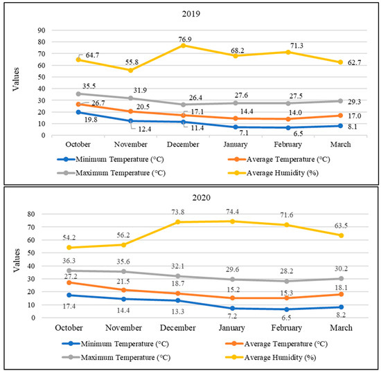
Figure 1.
Temperature and humidity conditions in the study area.
2.2. Plant Material and Nutrient Elements
The plant material used in the study was the Fieldglory F1 white head cabbage, which is suitable for cultivation during the summer and autumn months. The cabbage plants were planted on 18 October 2019 in the first year and on 26 October 2020 in the second year, with a row spacing of 50 cm and 40 cm between rows. The cabbage plants were fertilized with 10–20 kg da−1 N, 10–12 kg da-1 P2O5, and 18–20 kg da−1 K2O by fertigation, in accordance with the methodology proposed by Vural et al. [34].
2.3. Experimental Design and Treatments
A drip irrigation system was used, and the amount of irrigation water was calculated according to evaporation in the Class-A Evaporation Pan. Since evaporation and evapotranspiration are different, the amount of evaporation measured was reduced by keeping the crop coefficient (kc) low. Different irrigation levels were considered for conventional deficit irrigation (I-125, I-100, I-75, I-50) and partial root drying (PRD-125, PRD-100, PRD-75, PRD-50) (Table 2). In the conventional deficit irrigation treatments, laterals with drippers spaced 40 cm apart were placed in each row. In the PRD treatments, two laterals were placed in each row, with a dripper spacing of 80 cm between them. The cabbage seedlings were planted at a distance of 40 cm between the drippers on the row (Figure 2). The plots were 1.28 m2 in area and contained 10 plants each. Eight plants were included in the analysis, with the first and last plants in each row considered as side effects. The research was conducted over a 2-year period, during the autumn seasons of 2019 and 2020, with three replications according to the random plots experimental design.
Table 2.
Description of irrigation treatments.
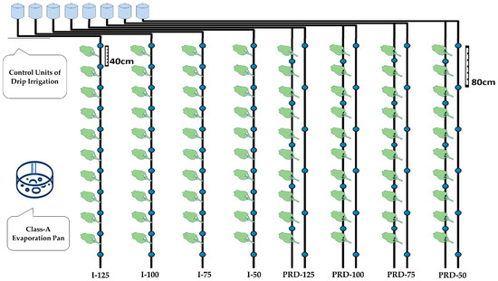
Figure 2.
Design of experimental plots according to irrigation treatments.
2.4. Irrigation Water Amount and Plant Water Consumption
From the planting of the cabbage seedlings in the greenhouse, each plant was provided with an equal amount of water until the commencement of root development. Afterwards, as suggested by Kirda et al. [35] and Topcu et al. [36], a Class-A Evaporation Pan was placed in the greenhouse and the amount of irrigation water applied to the I-100 treatment was calculated using the Equation (1) taking the evaporation measurements into account:
I = kp × kc × Ep × A
In the equation: I: irrigation water (l plant−1); kp: Class-A Evaporation Pan coefficient, 1 was taken; kc: the percentage cover value started from 0.30 and increased up to a coefficient of 0.45 depending on the plant development; Ep: total evaporation measured from the Class-A Evaporation Pan corresponding to the irrigation interval (mm); and A: area of a plant (m2).
The seasonal effect was considered in the study. In other words, in the first year of the study (2019), plant water consumption was low, and irrigation was scheduled not to exceed 0.20 L per plant. In the second year (2020), plant water consumption was higher, and irrigation was scheduled not to exceed 0.31 L per plant.
2.5. Evapotranspiration (ET), Water Use Efficiency (WUE), Irrigation Water Use Efficiency (IWUE), and Yield Response Factor (ky)
Plant evapotranspiration (ET) was calculated based on the water budget using the Equation (2):
In the equation: ET is the plant evapotranspiration (mm); I is the amount of irrigation water applied (mm); and ΔS is the change in water content between the beginning and the end of the season (mm).
There was no capillary water inflow as the study was carried out in an area with no groundwater problems. In addition, the study was conducted in the greenhouse, so the precipitation had no effect. For these reasons, capillary water inlet, surface runoff, and precipitation, etc., were not included in the plant evapotranspiration equation.
By calculating the plant evapotranspiration and recording the yield values, the water use efficiency (WUE) for each irrigation regime was calculated using the Equation (3):
In the equation: WUE is water use efficiency (kg m−3); Y is yield (kg da−1); and ET is plant evapotranspiration (mm).
Along with recording the irrigation water and yield values applied during the season, the efficiency of irrigation water use (IWUE) for each irrigation regime was calculated using the Equation (4):
In the equation: IWUE is the irrigation water usage efficiency (kg m−3); Y is the yield (kg da−1); and I is the irrigation water applied during the season (mm).
The yield response factor (ky) is an important parameter in the planning of irrigation applications. Ky, which is an indicator of the effect of water deficiency on plant yield, was calculated using the Equation (5) proposed by Doorenbos and Kassam [37] and Stewart et al. [38]:
In the equation: Ya is the actual yield (t ha−1), which corresponds to the actual plant evapotranspiration in the environments where the plant is cultivated; Ym is the yield obtained through maximum evapotranspiration in the environments where no water shortage is experienced through the growth season (t ha−1); ky is the yield response factor, which shows the decrease in the yield due to a unit decrease in the evapotranspiration; ETa is the actual evapotranspiration in environments where the plant is cultivated (mm); and ETm is the maximum evapotranspiration in environments where the plant is exposed to no water deficit through the growing season of the plant (mm).
2.6. Criteria Evaluated in the Study
In the study, head diameter (cm), head height (cm), stem diameter (mm), total and marketable yield (t ha−1) of cabbage, Lightness (L*), chroma (C*), and hue (h°) colour values of cabbage leaves were determined, and total soluble solids contents (SSC, %), pH, and titratable acidity (TA) criteria were analyzed in juices of cabbage leaves. In addition, water use efficiency (WUE, kg m−3) and irrigation water use efficiency (IWUE, kg m−3), evapotranspiration (mm), yield response factor (ky), and irrigation water amount (mm) values were determined according to total and marketable yield. To determine the marketable yield, the outer, inedible leaves of the lettuce were removed after harvest and the marketable yield was determined. L*, C*, h° colour values were measured with a Minolta CR400 colour chromameter, SSC digital refractometer [39]. TA was determined by the titration method and was expressed as g citric acid kg−1 [40].
2.7. Statistical Analysis
A statistical analysis was conducted using JMP Pro 17 software, which is part of the SAS program. This was employed to compare the data obtained from the various treatments and to perform an analysis of variance. The means were compared using the least significant difference (LSD) test. Furthermore, correlation coefficient-based analyses were conducted using MINITAB 21 software.
3. Results
3.1. Irrigation Water (I), Evapotranspiration (ET), Yield, Water Use Efficiency (WUE), Irrigation Water Use Efficiency (IWUE), and Yield Response Factor (ky)
The irrigation water (I, mm) and plant water consumption (ET, mm) values are given in Table 3. In the first year, a total of 29 irrigations were made, including life water, and 27 irrigations were made in the second year. However, in the second year, the water requirements of the plants increased due to the climatic conditions (Figure 1). This is because the average temperature in the second year was higher than in the first. As a result, the amount of irrigation water varied between 28.37 mm and 39.94 mm in the first season and between 32.32 mm and 46.40 mm in the second season (Table 3). ET values were calculated between 47.69 mm and 60.78 mm in the first season and between 80.11 mm and 101.37 mm in the second season (Table 3).
Table 3.
Amount of irrigation water and evapotranspiration in different treatments of the study.
As mentioned in the methods section, ET was calculated according to Equation (2). ET is one of the important parameters in water-yield relationships. When the ET values for four different irrigation levels (125%, 100%, 75%, and 50%) and the PRD technique were considered, as expected, they showed significant changes for both seasons. As seen in Table 3, for regions where water is scarce and expensive, it is important to consider 75% irrigation levels.
In general, a decrease in ET values was observed as the irrigation water level decreased. On the other hand, according to the data in Table 3, the increase in ET values in response to the irrigation program and the amount of water applied is the most important indicator that there is no deep infiltration (surface runoff was not observed anyway) and that the irrigation management is correct. This situation proves that water is used most efficiently in cabbage cultivation.
It was found that the values of total and marketable yield (t ha−1) were statistically affected by the irrigation program applied, and the details are given in Table 4. In the first season, the highest total yield of 124.40 t ha−1 was recorded in I-125 and the lowest yield of 94.53 t ha−1 was recorded in PRD-50. However, the yield values of I-125, I-100, I-75, PRD-125, and PRD-100 plots were statistically similar. In the second season, the highest total yield was found as 72.33 t ha−1 in PRD-125 and the lowest yield was found as 37.58 t ha−1 in I-50. Statistically, I-125, I-100, and PRD-125 subjects showed statistical similarity in terms of total yield (Table 4).
Table 4.
Total and marketable yield values.
The marketable yield values were calculated as follows: In the first season, the highest value was 91.93 t ha−1 in I-125 and the lowest value was 63.17 t ha−1 in PRD-50 treatment (Table 4). I-125, I-100, PRD-125, and PRD-100 subjects were in the same group with the highest marketable yield values. In the second season, the total highest value was 49.92 t ha−1 in PRD-125 while the lowest yield was 24.94 t ha−1 in I-50. However, I-125, I-100, and PRD-125 had statistically equal and the highest marketable yield values. In general, similar results were obtained for the irrigated treatments in terms of total and marketable yields. As the amount of irrigation water decreased (Table 3), a decrease in yield values (Table 4) was also observed.
Water use efficiency (WUE) and irrigation water use efficiency (IWUE) values were statistically influenced by irrigation programs and amount, and the results are shown in Table 5. The WUE and IWUE, which are the most important parameters and can be used to show the effectiveness of water-saving methods, played a very important role. In the study, there were changes in yield, evaporation, and water amounts due to seasonal effects that affected the WUE and IWUE values. For total yield, the highest WUE value (252.31 kg m−3) was calculated in PRD-100 and the lowest (185.19 kg m−3) in PRD-50 in the first year (Table 5). The highest WUE value (71.35 kg m−3) was found in PRD-125 and the lowest (44.90 kg m−3) in PRD-100 in the second year. For the marketable yield, the highest WUE value (182.65 kg m−3) was calculated in PRD-100 and the lowest (123.76 kg m−3) in PRD-50 in the first year (Table 5). In the second year, the highest WUE value (51.44 kg m−3) was found in I-100 and the lowest (30.36 kg m−3) in PRD-100.
Table 5.
WUE (kg m−3) and IWUE (kg m−3) values for the total and marketable product in different experimental treatments.
For total yield, the highest IWUE value (390.13 kg m−3) was calculated for I-50 in the first year and the lowest (309.88 kg m−3) was determined for PRD-125 (Table 5). The highest WUE value (155.89 kg m−3) was obtained for PRD-125 and the lowest (102.68 kg m−3) for PRD-100 in the second year. For the marketable yield, the highest IWUE value (273.20 kg m−3) was calculated for I-50 in the first year and the lowest (220.81 kg m−3) for PRD-125 (Table 5). The highest IWUE value (112.62 kg m−3) was recorded for I-100 and the lowest (69.43 kg m−3) for PRD-100 in the second year.
To more clearly demonstrate the water-yield relationships for cabbage in the study, visual representations of total and marketable yield, irrigation water, and evapotranspiration (ET) values are presented in Figure 3. The finding that evapotranspiration (ET) values were higher than the amount of irrigation water applied throughout the study provides compelling evidence that the water was used in an optimal manner, with no losses such as deep infiltration into the soil. The irrigation management was appropriate and effective. On the other hand, it was found that the reduction in the amount of irrigation water also led to a reduction in yield (Figure 3).
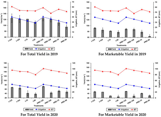
Figure 3.
Cabbage yield (t ha−1), irrigation water (mm), and ET (mm). The vertical line bars show means (n = 3) ± SD.
As illustrated in Figure 4, the correlation between conventional irrigation (I-125, I-100, I-75, and I-50) and yield demonstrated a notable increase in yield values (Table 4) with the application of increased irrigation water. This finding also lends support to the observed increase in water potential (IWUE) (Table 5, Figure 3).
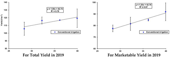
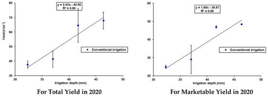
Figure 4.
Correlations between irrigation water (mm) and cabbage yield (t ha−1) in conventional irrigation.
As with Figure 4, the correlation between the PRD technology (PRD-125, PRD-100, PRD-75, and PRD-50) and yield can be observed in Figure 5. It can be generally stated that the observed increase in yield values (Table 4) is attributable to the increase in irrigation water. Furthermore, this resulted in an increase in the IWUE values (Table 5, Figure 3). While not identical to Figure 4 and Figure 5, it is evident that the relationship between evapotranspiration (ET, mm) and yield (t ha−1) is influenced by the quantity of irrigation water applied (Figure 6 and Figure 7).
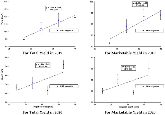
Figure 5.
Correlations between irrigation water (mm) and cabbage yield (t ha−1) in partial root drying irrigation.
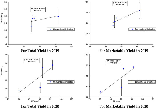
Figure 6.
Correlations between evapotranspiration (ET, mm) and cabbage yield (t ha−1) in conventional irrigation.
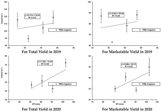
Figure 7.
Correlations between evapotranspiration (ET, mm) and cabbage yield (t ha−1) in partial root drying irrigation.
“ky” values were calculated as an indicator of the effect of the proportional decrease in plant water use (ET) on the proportional decrease in cabbage yield. The relationship between seasonal plant water use and yield values was determined using regression analysis (Figure 8). As in Table 4, Figure 3, Figure 6 and Figure 7, the decrease in yield values was generally found to be significant in response to the decrease in ET values (Figure 8).
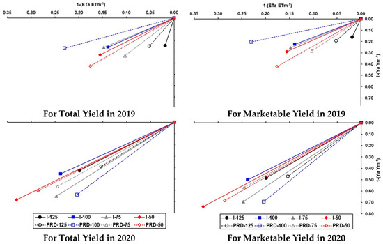
Figure 8.
Relative cabbage yield reduction as a function of relative ET deficit.
3.2. Cabbage Head Height, Head Diameter, and Stem Diameter
The effects of different irrigation levels on cabbage head height, head diameter, and stem diameter (Figure 9) were statistically significant in both growth periods (p < 0.05). For head height and head diameter, I-125 gave the highest values in the first year, I-125 and PRD-125 in the second year. For head height, the I-125 treatment gave an increase of 0.6% and 2.3%, respectively, over the control (I-100) in both growth periods, while for head diameter, the I-125 treatment gave an increase of 2.1% over I-100 in the first year and 7.6% in the second year. Furthermore, the plants cultivated during the first year exhibited greater height and width than those cultivated during the subsequent year, particularly in terms of head height and diameter. With regard to stem diameter, the PRD treatments (PRD-125, PRD-100, and PRD-75) exhibited higher values than the other irrigation treatments in the first year, whereas the I treatments (I-125, I-100, and PRD-125) demonstrated higher values in the second year. The deficit irrigation treatment (PRD-75) exhibited values that were 6.4% higher than those observed for the control treatment (I-100) during the first year. The deficit irrigation treatment PRD-75 had 6.4% higher values than I-100 in the first year. In the second year, I-100 and I-125 together with PRD-125 showed similar responses. The PRD-50 treatment had the lowest stem diameter values in both years.
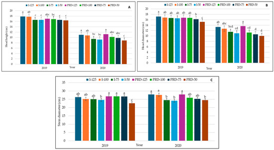
Figure 9.
Effects of different irrigation levels on head height (A), head diameter (B), and stem diameter (C) of cabbage plants in the first and second years of the study. (Columns with different letters indicate the significance at p < 0.05 levels).
3.3. L*, C*, and h° Colour Values of Cabbage Leaves
There were significant differences between L* and C* colour values of cabbage leaves in both growth periods according to different irrigation levels (except h°) (Table 6). The numerical L* value was highest in the PRD-50 treatment in both the first and second years. For the C* colour value, the highest value was found in PRD-125 in the first year and in I-125 in the second year. The hue angle values, which did not show significant differences, varied between 128.14–132.48 in the first year and 132.28–139.76 in the second year.
Table 6.
Effects of different irrigation levels on colour values in cabbage plants.
3.4. Soluble Solid Contents, pH, and Titratable Acidity in Cabbage Juices
The effect of the different irrigation regimes on the soluble solids contents in cabbage leaf juices was significant (Table 7). In both growth periods, the highest soluble solids were recorded in PRD-50, with values of 8.74% and 12.85%, respectively. A comparison of these values with I-100 revealed an increase in SSC of 16.06% and 36.27%, respectively. While no significant difference was observed in the pH values of the lettuce juices in the first year, significant differences were evident between the treatments in the second year. The pH of the lettuce juices in the PRD-125 treatments was the highest, while the other treatments exhibited no statistically significant differences. With regard to titratable acidity, the various irrigation regimes had no significant impact.
Table 7.
Effects of different irrigation levels on SSC, pH, and TA in cabbage juices.
3.5. Pearson Correlation Analyses
The positive or negative proportional effect of different irrigation applications on the criteria studied in cabbage was evaluated using Pearson correlation analysis (p < 0.05). In the correlation analysis, the mean values of the studied criteria according to the treatments were used. The correlation analysis and its coefficients are shown in Figure 10.
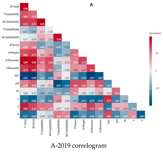
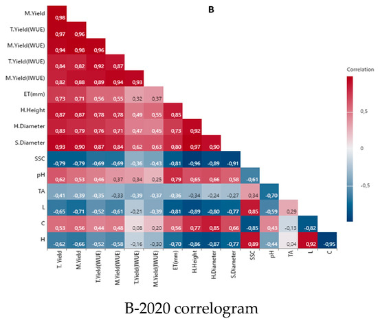
Figure 10.
Results of the correlation analysis of the criteria examined in the study for the year 2019 (A) and the year 2020 (B).
Correlation coefficients showed a positive relationship between total yield and marketable yield, head diameter and C color parameters, stem diameter, and WUE for the first-year marketable yield. However, there was a negative relationship between total yield and SSC, L* and h∘ color parameters. While a positive relationship was determined between marketable yield and head and stem diameter, WUE for marketable yield and head height, a negative relationship was determined with SSC, L*, and h° color parameters. WUE for total yield had a strong positive relationship with WUE for marketable yield. IWUE for total yield had a strong positive relationship with IWUE for marketable yield. However, its relationship with pH was strong and negative. IWUE determined for marketable yield had a significant negative relationship only with pH of cabbage juices. Similarly, a negative relationship was determined for ET with H color parameter. Head height was related to stem diameter (positive) and colour parameter L (negative), stem diameter was related to colour parameters SSC (negative), L* (negative), and C (positive), stem diameter was related to SSC (negative) and L* (negative), SSC was related to L (positive), and colour parameter C (negative) was related to h°.
Upon evaluation of the significance of the correlation for the second year in terms of the parameters studied, it was observed that there were mutually strong positive relationships between marketable yield, WUE, and IWUE for total and marketable yield. ET appeared to have a positive relationship with total and marketable yield. It would appear that head height had a positive relationship with total and marketable yield, as well as with their WUE-IWUE and ET. As shown in Figure 10, head diameter, stem diameter, and pH had some positive significant relationships. SSC had negative significant relationships with some other parameters. While the significant relationships of L* color parameter were negative, its relationship with SSC was a strong positive relationship. There were also positive and negative relationships for C* and h° color parameters.
3.6. Principle Component Analysis (PCA)
Principal component analyses were performed on the criteria examined in the study over a 2-year period (Figure 11). The results of the investigation were analyzed in order to ascertain whether there were any notable differences in the averages of the various criteria according to the different irrigation regimes. The colors of the arrows on the graphs indicate the parameters with negative and positive loads included in the components. The graph shows two components for the first and second years. Although two components are shown in the second year, the parameter of the third component with the third higher load is also included in the graph. The red color indicates the first component, the blue colour indicates the second component and the green color indicates the third component. In the PCA carried out in the first year (Figure 11A), it can be seen that the first principal component accounts for 52.4%, the second principal component 23.6%, and the total variation 76%. In the PCA carried out in the second year (Figure 11B), the first component reached 68.9%, the second component reached 15.8%, and the total variation reached 84.7%.
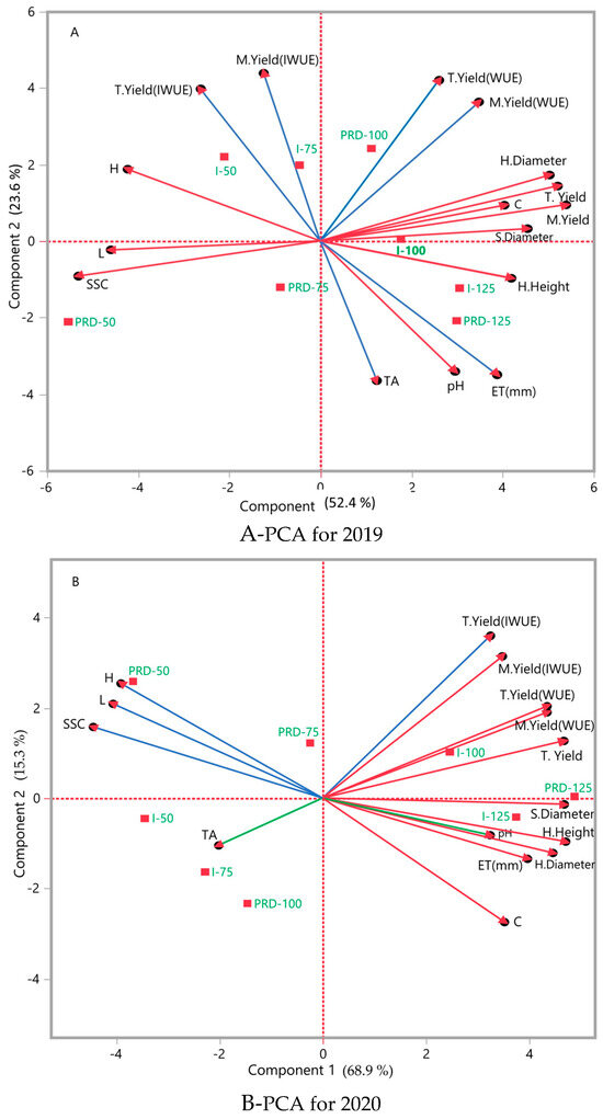
Figure 11.
Principal component analyses of the criteria examining the effects of different irrigation practices for 2019 (A) and 2020 (B).
In the first year of the research, the first component included marketable yield, total yield, head diameter, stem diameter, head height, C* colour, pH, and water use efficiency according to marketable yield criteria according to factor loadings, while the second component included irrigation water use efficiency according to marketable yield, irrigation water use efficiency according to total yield, and water use efficiency according to marketable yield. In the PCA analysis conducted for the second year of the research, the first component consisted of the following factors: head height, stem diameter, total yield, marketable yield, head diameter, water use efficiency by total yield, water use efficiency by marketable yield, total evaporation, chroma colour value, irrigation water use efficiency by marketable yield, irrigation water use efficiency by total yield, and pH criteria. In the second component, irrigation water use efficiency by total yield, irrigation water use efficiency by marketable yield, and h colour value came to the fore. In both the first and second years of the study, the SSC, L*, and h° parameters in the component were the ones with strong negative loadings.
4. Discussion
Recent climate change and drought have highlighted the importance of water use in vegetable production. The main objective of crop production is to achieve the highest yield and quality. Therefore, it is of great importance to produce vegetables with less irrigation water without losing yield and quality [41]. There are many studies on traditional deficit irrigation and water-saving applications known as partial root drying (PRD).
In our study, conventional deficit irrigation (I-125, I-100, I-75, I-50) and PRD techniques were compared in cabbage production, as also mentioned by Sadras [21]. Although there are studies on conventional deficit irrigation in cabbage, PRD technique in cabbage was investigated in very few studies so far. This study has attracted attention in this regard. In this study, the yield values of cabbage were affected by different irrigation water levels. In the first year, the highest total yield values were recorded in I-125 and PRD-125. In the second year, this was followed by PRD-125, I-125, and I-100. In the first year, the marketable yield was highest in I-125, PRD-125, and PRD-100, while in the second year, it was highest in PRD-125, I-125, and I-100. As anticipated, the lowest numerical yield was observed in I-50 and PRD-50, which received the least irrigation water. The analysis of variance indicates that the yield values in the I-75 and PRD-75 treatments are comparable to those in I-100 and PRD-100. Although the yield values obtained for the first and second years were parallel according to the irrigation treatments, the yield values were lower in the second year. The reason for this was that temperatures above seasonal norms were observed during the vegetative development of the cabbage plants in the second year. Therefore, it is assumed that the plants could not benefit from the irrigation water, despite the fact that more water was given to the plants due to increased evapotranspiration.
The results of some studies investigating different irrigation levels are in parallel with our results. For example, Xu and Leskovar [42] obtained the highest cabbage yield with 100% irrigation using the conventional deficit irrigation technique. Saha et al. [43] obtained the highest head yield in 25% soil moisture reduction and full irrigation treatments, and higher ET was determined with the higher irrigation regime. The results of the water-yield relationship are consistent with our study, and similar results were observed in some other studies [43,44,45]. There is no study investigating the response of cabbage plants to PRD in cabbage.
It is worth noting that there were statistically significant differences in WUE and IWUE values. Differences in WUE and IWUE were found between irrigation treatments and years. It was particularly noteworthy that WUE and IWUE reached the highest values for total and marketable yield in the deficit irrigation treatments PRD-75, PRD-50, I-75, and I-50. This indicates that satisfactory yields can be achieved with less irrigation under water-scarcity conditions. There are similar and different results in some previous studies. Buyukcangaz [25] evaluated that variety selection, climate, and soil structure may affect the differences in WUE and IWUE over the years. In a 2-year study on cauliflower by Abdelkhalik et al. [12], a 37% difference in productivity was found between years with irrigation strategies similar to our study, so IWUE was higher with more irrigation in the year when yield decreased. Although there was no difference in yield between water-stress applications, the highest effect in terms of IWUE was found in the highest water-stress application (50%). Ayas et al. [46] obtained the highest yield with full irrigation, while when irrigation water was reduced by 25%, similar yield values were obtained and the highest WUE was determined. Seymen et al. [47] observed that the highest yield was achieved through the application of full irrigation in cauliflower. While there was a correlation between the amount of water applied and the WUE values, it is notable that the lowest value was observed in the highest water-stress application (60%). Buyukcangaz and Ayas [48] obtained the highest total yield of cauliflower with full irrigation, while marketable yield was obtained with full and 25% reduced irrigation. The highest WUE and IWUE were obtained with the 25% reduced application. Although there is no research on PRD in cabbage, in lettuce, a cool-climate vegetable whose leaves are consumed like cabbage, Demir et al. [49] reported that total and marketable yields were similar under regular deficit irrigation and PRD applications and varied with the amount of irrigation water. Under the PRD technique, some vegetables such as tomato [35,50,51], cucumber [52], pepper [53], capia pepper [54], and eggplant [55] were comparatively studied with conventional deficit irrigation and PRD techniques, and the water-yield relationships of cabbage were similar to the results of these vegetables.
This study suggests that the growth characteristics of cabbage may be influenced by irrigation treatments, with results that appear to align with those of previous studies. For instance, Seymen et al. [44] have suggested that water deficiency may potentially lead to notable reductions in the growth of cabbage plants. Buyukcangaz and Ayas [48] obtained values from a full dose with 25% water restriction in the head height of cauliflower in a 2-year study. It would seem that the highest value in terms of head diameter was obtained from the full dose. Similar results were obtained from broccoli by Ayas et al. [46]. Çerez and Şahin [56] observed that the head diameter of lettuce was comparable to the full dose and 120% irrigation when a 20% water restriction was applied. Xu and Leskovar [42] observed a moderate reduction in head height and head width when irrigation was applied at 75% of evapotranspiration. In a study where irrigation was applied according to soil moisture loss, it was observed that head height and head diameter of cabbage reached maximum values at 0% and 25% evaporation. Abdelkhalik et al. [12] observed that a 50% reduction in water intake during the juvenile stage of cauliflower resulted in reduced crown formation and plant size. Furthermore, when the same 50% water restriction was applied throughout the growing season, crown size was found to be significantly reduced. Souza et al. [57] reported that plant height and leaf number of cauliflower decreased under 40% water stress compared to higher irrigation levels.
Acar et al. [58] reported that the differences in head height and head diameter were not significant between 40% and 20% water-deficit conditions and full irrigation, but SSC was higher under full irrigation. Chen et al. [59] reported that SSC of tomato increased with decreasing water application. Blanch et al. [60] measured SSC approximately 2 and 1 times higher in lettuce exposed to severe and moderate water deficits, respectively, compared to the control. Bozkurt Çolak et al. [61] found that SSC increased with decreasing irrigation in eggplant in both DI and PRD treatments. Casa and Rouphael [50] found that DI and PRD treatments in tomato increased TA and Brix, but there were no significant differences in pH. Although there were no statistically significant differences between irrigation regimes, when titratable acid concentrations were compared with one another in the first year of the study, there was a slight numerical increase in PRD applications. Sun et al. [62] and Xu et al. [63] found that titratable acid concentrations in tomatoes were higher in PRD applications. Kuşçu et al. [64] determined that different irrigation levels in watermelon juices did not affect SSC and pH, and titratable acidity levels increased as water restriction increased. Demirel et al. [65] determined that pH and SSC were higher in applications where 33% of usable water was given, and no irrigation was applied to capia pepper compared to other irrigation levels.
In both years of the study, the L values read on cabbage leaves increased as deficit irrigation increased. This may be related to the increase in the waxy layer on the leaves. Because the waxy layer increased with drought stress and this turned into a white color, the L value was high. The C value, which expresses the tone of the green color, was determined at the lowest PRD-50. In terms of color tone, the plants in 75% conventional water deficit and full irrigation were similar. Abdelkhalik et al. [12] found a similar result for the L value in cauliflower and noted that it increased the marketability of cauliflower, but the C and ho values were lower. PCA is a statistical tool used to interpret the measured values according to stress factors. There are many previous studies on abiotic stress [66], water-yield relationship under deficit irrigation conditions, and determination of biochemical properties [1,44,67].
5. Conclusions
The study indicated that the irrigation treatments had a notable impact on both the total and marketable cabbage yields in both growing seasons. It is worth noting that the ET values were found to be higher than the amount of irrigation water applied throughout the study. This suggests that the water was used effectively, with minimal losses such as deep infiltration in the soil. It would seem that the highest total and marketable yields were found in the I-125, PRD-125, I-100, and PRD-100 treatments. As a general observation, it seems that a reduction in the volume of irrigation water has resulted in a corresponding decline in yield.
Although cabbage growth characteristics varied between years, in general the I-125, PRD-125, I-100, PRD-100, I-75, and PRD-75 treatments gave better results. It was found that as deficit irrigation increased, the waxy layer on cabbage leaves increased, which increased the L value. It was also measured that SSC increased with increasing deficit irrigation. The fact that the partial root drying (PRD) technique has not been considered in previous studies, especially for cabbage, significantly increases the original value of this study. The main purpose of the PRD technique is to increase water use efficiency without reducing yield. It was important that WUE and IWUE values reached their highest levels in full irrigation and 25% more irrigation treatments as well as in deficit irrigation treatments. If there is a need to reduce irrigation water, I-75 and PRD-75 are also recommended. However, if the percentage of “kc” plant coefficient cover is increased, it is predicted that I-50 and PRD-50 subjects may also provide advantages. In conclusion, the research suggests that further irrigation-yield relationships would be beneficial.
Author Contributions
Conceptualization, H.D., H.K., İ.S. and İ.H.A.; Data curation, H.D., H.K., İ.S., İ.H.A. and U.U.; Formal analysis, H.D. and İ.S.; Funding acquisition, H.D., H.K., İ.S., İ.H.A. and U.U.; Investigation, H.D., H.K., İ.H.A. and U.U; Methodology, H.D., H.K., İ.S., İ.H.A. and U.U.; Project administration, H.D. and H.K.; Resources, H.D. and H.K.; Writing—original draft preparation, H.D., İ.S. and H.K.; Writing—review and editing, H.D., H.K. and İ.S.; Supervision, H.D. and H.K. All authors have read and agreed to the published version of the manuscript.
Funding
This research received no external funding.
Data Availability Statement
Data related to the research are reported in the paper. Any additional data may be acquired from the first corresponding author upon request.
Conflicts of Interest
The authors declare no conflict of interest.
References
- Yavuz, D.; Seymen, M.; Yavuz, N.; Çoklar, H.; Ercan, M. Effects of water stress applied at various phenological stages on yield, quality, and water use efficiency of melon. Agric. Water Manag. 2021, 246, 106673. [Google Scholar] [CrossRef]
- Nadeem, M.; Li, J.; Yahya, M.; Sher, A.; Ma, C.; Wang, X.; Qiu, L. Research progress and perspective on drought stress in legumes: A review. Int. J. Mol. Sci. 2019, 20, 2541. [Google Scholar] [CrossRef] [PubMed]
- Tester, M.; Langridge, P. Breeding technologies to increase crop production in a changing world. Science 2010, 327, 818–822. [Google Scholar] [CrossRef] [PubMed]
- Hatamian, M.; Rezaei Nejad, A.; Kafi, M.; Souri, M.K.; Shahbazi, K. Growth characteristics of ornamental Judas tree (Cercis siliquastrum L.) seedling under different concentrations of lead and cadmium in irrigation water. Acta Sci. Pol. Hortorum Cultus 2019, 18, 87–96. [Google Scholar] [CrossRef]
- Ebrahimi, M.; Souri, M.K.; Mousavi, A.; Sahebani, N. Biochar and vermicompost improve growth and physiological traits of eggplant (Solanum melongena L.) under deficit irrigation. Chem. Biol. Technol. Agric. 2021, 8, 19. [Google Scholar] [CrossRef]
- Bute, A.; Iosob, G.A.; Antal-Tremurıcı, A.; Brezeanu, C.; Brezeanu, P.M.; Crıstea, T.O.; Ambăruș, S. The Most Suitable Irrigation Methods in Cabbage Crops (Brassica oleracea var. capitata): A review. Sci. Papers. Ser. B Hortic. 2021, LXV, 399–405. [Google Scholar]
- Jiménez-Ariasa, D.; García-Machado, F.J.; Morales-Sierra, S.; Luis, J.C.; Suarez, E.; Hernández, M.; Valdés, F.; Borges, A.A. Lettuce plants treated with L-pyroglutamic acid increase yield under water deficit stress. Environ. Exp. Bot. 2019, 158, 215–222. [Google Scholar] [CrossRef]
- Souri, M.K.; Römheld, V. Split daily applications of ammonium cannot ameliorate ammonium toxicity in tomato plants. Hortic. Environ. Biotechnol. 2009, 50, 384–391. [Google Scholar]
- Souri, M.K.; Hatamian, M. Aminochelates in plant nutrition: A review. J. Plant Nutr. 2019, 42, 67–78. [Google Scholar] [CrossRef]
- Hatamian, M.; Rezaei Nejad, A.; Kafi, M.; Souri, M.K.; Shahbazi, K. Nitrate improves hackberry seedling growth under cadmium application. Heliyon 2020, 6, e03247. [Google Scholar] [CrossRef]
- Fereres, E.; Soriano, M.A. Deficit irrigation for reducing agricultural water use. J. Exp. Bot. 2007, 58, 147–159. [Google Scholar] [CrossRef]
- Abdelkhalik, A.; Pascual, B.; Nájera, I.; Baixauli, C.; Pascual-Seva, N. Deficit Irrigation as a Sustainable Practice in Improving Irrigation Water Use Efficiency in Cauliflower under Mediterranean Conditions. Agronomy 2019, 9, 732. [Google Scholar] [CrossRef]
- Chai, Q.; Gan, Y.; Zhao, C.; Xu, H.L.; Waskom, R.M.; Niu, Y.; Siddique, K.H.M. Regulated deficit irrigation for crop production under drought stress. A review. Agron. Sustain. Dev. 2016, 36, 3. [Google Scholar] [CrossRef]
- Capra, A.; Consoli, S.; Scicolone, B. Deficit irrigation: Theory and practice. In Agricultural Irrigation Research Progress; Chapter: 4; Alonso, D., Iglesias, H.J., Eds.; Nova Science Publishers, Inc.: New York, USA, 2008; pp. 53–82. [Google Scholar]
- Giuliani, M.M.; Gatta, G.; Nardella, E.; Tarantino, E. Water saving strategies assessment on processing tomato cultivated in Mediterranean region. Ital. J. Agron. 2016, 11, 69–76. [Google Scholar] [CrossRef]
- English, M.J.; Raja, S.N. Perspectives on deficit irrigation. Agric. Water Manag. 1996, 32, 1–14. [Google Scholar] [CrossRef]
- Hernandez-Santana, V.; Fernández, J.E.; Cuevas, M.V.; Perez-Martin, A.; Diaz-Espejo, A. Photosynthetic limitations by water deficit: Effect on fruit and olive oil yield, leaf area and trunk diameter and its potential use to control vegetative growth of super-high-density olive orchards. Agric. Water Manag. 2017, 184, 9–18. [Google Scholar] [CrossRef]
- Padilla-Díaz, C.M.; Rodriguez-Dominguez, C.M.; Hernandez-Santana, V.; Perez-Martin, A.; Fernández, J.E. Scheduling regulated deficit irrigation in a hedgerow olive orchard from leaf turgor pressure related measurements. Agric. Water Manag. 2016, 164, 28–37. [Google Scholar] [CrossRef]
- Zegbe, J.A.; Behbouidan, M.H.; Clothier, B.E. Responses of ‘Petopride’ processing tomato to partial rootzone drying at different phenological stages. Irrig. Sci. 2006, 24, 203–210. [Google Scholar] [CrossRef]
- Ahmadi, S.H.; Andersen, M.N.; Plauborg, F.; Poulsen, R.T.; Jensen, C.R.; Sepaskhah, A.R.; Hansen, S. Effects of irrigation strategies and soils on field grown potatoes: Gas exchange and xylem (ABA). Agric. Water Manag. 2010, 97, 1486–1494. [Google Scholar] [CrossRef]
- Sadras, V.O. Does partial root-zone drying improve irrigation water productivity in the field? A meta-analysis. Irrig. Sci. 2009, 27, 183–190. [Google Scholar] [CrossRef]
- Savic, S.; Liu, F.; Stikic, R.; Jacobsen, S.E.; Jensen, C.R.; Jovanovic, Z. Comparative effects of partial root-zone drying and deficit irrigation on growth and physiology of tomato plants. Arch. Biol. Sci. 2009, 61, 801–810. [Google Scholar] [CrossRef]
- Kirda, C.; Topcu, S.; Cetin, M.; Dasgan, H.Y.; Kaman, H.; Topaloglu, F.; Derici, M.R.; Ekici, B. Prospects of partial root-zone irrigation for increasing irrigation water use efficiency of major crops in the Mediterranean region. Ann. Appl. Biol. 2007, 150, 281–291. [Google Scholar] [CrossRef]
- Ismail, M.R.; Phizackerley, S. Effects of partial rootzone and controlled deficit irrigation on growth, yield and peroxidase activity of tomatoes (Lycopersicon esculentum Mill.). Intern. J. Agric. Res. 2009, 4, 46–52. [Google Scholar] [CrossRef][Green Version]
- Buyukcangaz, H. Deficit Irrigation Effects on Cabbage (Brassicaceae oleracea var. capitata L. Grandslam F1) Yield in Unheated Greenhouse Condition. Turk. J. Agric. Food Sci. Technol. 2018, 6, 1251–1257. [Google Scholar] [CrossRef][Green Version]
- Nikzad, M.; Aravinda Kumar, J.S.; Anjanappa, M.; Amarananjundeswara, H.; Dhananjaya, B.N.; Basavaraj, G. Effect of fertigation, levels on growth and yield of cabbage (Brassica oleracea L. var. capitata). Int. J. Curr. Microbiol. App. Sci. 2020, 9, 1240–1247. [Google Scholar] [CrossRef]
- Hasan, M.R.; Sani, M.N.H.; Tahmina, E.; Uddain, J. Growth and yield responses of cabbage cultivars as influenced by organic and inorganic fertilizers. Asian Res. J. Agric. 2018, 9, 1–12. [Google Scholar] [CrossRef]
- Adeniran, K.A.; Amodu, M.F.; Amodu, M.O.; Adeniji, F.A. Water requirements of some selected crops in Kampe dam irrigation project. Aust. J. Agric. Eng. 2010, 1, 119–125. [Google Scholar]
- Nyatuame, M.; Ampiaw, F.; Owusu-Gyimah, V.; Ibrahim, B. M. Irrigation scheduling and water use efficiency on cabbage yield. Int. J. Agron. Agri. Res. 2013, 3, 29–35. [Google Scholar]
- FAO. Crops and Livestock Products. 2022. Available online: https://www.fao.org/faostat/en/#data/QCL (accessed on 16 October 2024).
- TUIK. Bitkisel Üretim İstatistikleri. 2023. Available online: https://data.tuik.gov.tr/Bulten/Index?p=Bitkisel-Uretim-Istatistikleri-2023-49535 (accessed on 16 October 2024).
- Kacar, B. Bitki ve toprağın kimyasal analizler: III. Toprak Analizleri. In Ankara Üniversitesi Ziraat Fakültesi; Araştırma ve Geliştirme Vakfı Yayınları: Ankara, Türkiye, 1995; Volume 3, p. 705. (In Turkish) [Google Scholar]
- Kacar, B.; Kovancı, D. Bitki, toprak ve gübrelerde kimyasal fosfor analizleri ve sonuçlarinin değerlendirilmesi. In Ege Üniversitesi Ziraat Fakültesi Yayınları; Ege University Faculty of Agriculture Publications: İzmir, Türkiye, 1982; p. 352. (In Turkish) [Google Scholar]
- Vural, H.; Esiyok, D.; Duman, I. Kültür Sebzeleri (Sebze Yetiştirme). In Cultured Vegetables (Growing Vegetables); Ege University Press: Bornova, İzmir, 2000; p. 440. (In Turkish) [Google Scholar]
- Kirda, C.; Cetin, M.; Dasgan, Y.; Topcu, S.; Kaman, H.; Ekici, B.; Derici, M.R.; Ozguven, A.I. Yield response of greenhouse grown tomato to partial root drying and conventional deficit irrigation. Agric. Water Manag. 2004, 69, 191–201. [Google Scholar] [CrossRef]
- Topcu, S.; Kirda, C.; Dasgan, Y.; Kaman, H.; Cetin, M.; Yazici, A.; Bacon, M.A. Yield response and N-fertiliser recovery of tomato grown under deficit irrigation. Eur. J. Agron. 2007, 26, 64–70. [Google Scholar] [CrossRef]
- Doorenbos, J.; Kassam, A.H. Yield Response to Water; Paper No. 33; FAO Irrigation and Drainage: Rome, Italy, 1979; p. 193. [Google Scholar]
- Stewart, J.I.; Cuenca, R.H.; Pruitt, W.O.; Hagan, R.M.; Tosso, J. Determination and Utilization of Water Production Functions for Principal California Crops; W67 CA Contributing Project Report; University of California: Davis, CA, USA, 1977. [Google Scholar]
- Siomas, A.S.; Papadopoulou, P.P.; Gogras, C.C. Quality of Romaine and Leaf Lettuce at Harvest and during Storage. Proc.2nd Balkan Symposium on Vegetables and Potatoes. Acta Hortic. 2002, 579, 641–646. [Google Scholar] [CrossRef]
- Kurubas, M.S.; Maltas, A.S.; Dogan, A.; Kaplan, M.; Erkan, M. Comparison of organically and conventionally produced Batavia type lettuce stored in modified atmosphere packaging for postharvest quality and nutritional parameters. J. Sci. Food Agric. 2019, 99, 226–234. [Google Scholar] [CrossRef] [PubMed]
- Yuan, B.Z.; Sun, J.; Nishiyama, S. Effect of drip irrigation on strawberry growth and yield inside a plastic greenhouse. Biosyst. Eng. 2004, 87, 237–245. [Google Scholar] [CrossRef]
- Xu, C.; Leskovar, D.I. Growth, physiology and yield responses of cabbage to deficit irrigation. Hortic. Sci. 2014, 41, 138–146. [Google Scholar] [CrossRef]
- Saha, C.; Bhattacharya, P.; Sengupta, S.; Dasgupta, S.; Patra, S.K.; Bhattacharyya, K.; Dey, P. Response of cabbage to soil test-based fertilization coupled with different levels of drip irrigation in an inceptisol. Irrig. Sci. 2022, 40, 239–253. [Google Scholar] [CrossRef]
- Seymen, M.; Yavuz, D.; Eroğlu, S.; Arı, B.Ç.; Tanrıverdi, Ö.B.; Atakul, Z.; Issı, N. Effects of Different Levels of Water Salinity on Plant Growth, Biochemical Content, and Photosynthetic Activity in Cabbage Seedling UnderWater-Deficit Conditions. Gesunde Pflanz. 2023, 75, 871–884. [Google Scholar] [CrossRef]
- Sabah, S.H.; Karim, T.H.; Tahir, H.T. Effect of Deficit Irrigation with Saline Water on Chemical Properties for Red Cabbage (Brassica oleracea var. capitata L.) under Drip Irrigation. Al-Qadisiyah J. Agric. Sci. 2023, 13, 28–39. [Google Scholar]
- Ayas, S.; Orta, H.; Yazgan, S. Deficit irrigation effects on broccoli (Brassica oleracea L. var. Monet) yield in unheated green-house condition. Bulg. J. Agric. Sci. 2011, 17, 551–559. [Google Scholar]
- Seymen, M.; Erçetin, M.; Yavuz, D.; Kıymacı, G.; Kayak, N.; Mutlu, A.; Kurtar, E.S. Agronomic and physio-biochemical responses to exogenous nitric oxide (NO) application in cauliflower under water stress conditions. Sci. Hortic. 2024, 331, 113116. [Google Scholar] [CrossRef]
- Buyukcangaz, H.; Ayas, S. Deficit irrigation effects on cauliflower (Brassica oleracea L. var. Skywalker F1) yield under unheated greenhouse conditions. Fresenius Environ. Bull. 2019, 28, 1775–1784. [Google Scholar]
- Demir, H.; Kaman, H.; Sönmez, İ.; Mohamoud, S.S.; Polat, E.; Üçok, Z. Yield, quality and plant nutrient contents of lettuce under different deficit irrigation conditions. Acta Sci. Pol. Hortorum Cultus 2022, 21, 115–129. [Google Scholar] [CrossRef]
- Casa, B.R.; Rouphael, Y. Effects of partial root-zone drying irrigation on yield, fruit quality, and water-use efficiency in processing tomato. J. Hortic. Sci. Biotech. 2014, 89, 389–396. [Google Scholar] [CrossRef]
- Giuliani, M.M.; Nardella, E.; Gagliardi, A.; Gatta, G. Deficit Irrigation and Partial Root-Zone Drying Techniques in Processing Tomato Cultivated under Mediterranean Climate Conditions. Sustainability 2017, 9, 2197. [Google Scholar] [CrossRef]
- Kaman, H.; Özbek, Ö.; Polat, E. Response of greenhouse grown cucumber to partial root zone drying and conventional deficit irrigation. Kahramanmaraş Sütçü İmam Univ. J. Agric. Nat. 2022, 25, 337–347. [Google Scholar]
- Bozkurt Çolak, Y.; Yazar, A.; Yıldız, M.; Tekin, S.; Gönen, E.; Alghawry, A. Assessment of crop water stress index and net benefit for surface- and subsurface-drip irrigated bell pepper to various deficit irrigation strategies. J. Agric. Sci. 2023, 161, 254–271. [Google Scholar] [CrossRef]
- Sezen, S.M.; Yazar, A.; Tekin, S. Physiological response of red pepper to different irrigation regimes under drip irrigation in the Mediterranean region of Turkey. Sci. Hortic. 2019, 245, 280–288. [Google Scholar] [CrossRef]
- Bozkurt Çolak, Y.; Yazar, A.; Sesveren, S.; Çolak, İ. Evaluation of yield and leaf water potantial (LWP) for eggplant undervarying irrigation regimes using surface and subsurface drip systems. Sci. Hortic. 2017, 219, 10–21. [Google Scholar] [CrossRef]
- Çerez, N.E.; Şahin, M. Effects of Irrigation Water Levels on Lettuce Yield and Water Use Efficiencies under Unheated Greenhouse Conditions. Gesunde Pflanz. 2022, 75, 1315–1324. [Google Scholar] [CrossRef]
- Souza, A.P.; da Silva, A.C.; Tanaka, A.A.; de Souza, M.E.; Pizzatto, M.; Felipe, R.T.A.; Martim, C.C.; Ferneda, B.G.; da Silva, S.G. Yield and water use efficiency of cauliflower under irrigation different levels in tropical climate. Afr. J. Agric. Res. 2018, 13, 1621–1632. [Google Scholar]
- Acar, B.; Paksoy, M.; Türkmen, Ö.; Seymen, M. Irrigation and nitrogen level affect lettuce yield in greenhouse condition. Afr. J. Biotechnol. 2008, 7, 4450–4453. [Google Scholar]
- Chen, J.; Kang, S.; Du, T.; Qiu, R.; Guo, P.; Chen, R. Quantitative response of greenhouse tomato yield and quality to water deficit at different growth stages. Agric. Water Manag. 2013, 129, 152–162. [Google Scholar] [CrossRef]
- Blanch, M.; Dolores Alvarez, M.; Sanchez-Ballesta, M.T.; Escribano, M.I.; Merodio, C. Water relations, short-chain oligosaccharides and rheological properties in lettuces subjected to limited water supply and low temperature stress. Sci. Hortic. 2017, 225, 726–735. [Google Scholar] [CrossRef]
- Bozkurt Çolak, Y.; Yazar, A.; Gönen, E.; Eroğlu, E.Ç. Yield and quality response of surface and subsurface drip-irrigated eggplant and comparison of net returns. Agric. Water Manag. 2018, 206, 165–175. [Google Scholar] [CrossRef]
- Sun, Y.; Holm, P.E.; Liu, F. Alternate partial root-zone drying irrigation improves fruit quality in tomatoes. Hortic. Sci. 2014, 41, 185–191. [Google Scholar] [CrossRef]
- Xu, H.L.; Qin, F.F.; Du, F.L.; Xu, Q.C.; Wang, R.; Shah, R.P.; Zhao, A.H.; Li, F.M. Application of xerophytophysiology in plant production—Partial root drying improves tomato crops. J. Food Agric. Environ. 2009, 7, 981–988. [Google Scholar]
- Kuşçu, H.; Turhan, A.; Özmen, N.; Aydınol, P.; Demir, A.O. Effects of different irrigation regimes on water use efficiency, yield and fruit quality of watermelon under Bursa ecological conditions. Mediterr. Agric. Sci. 2015, 28, 21–26. [Google Scholar]
- Demirel, K.; Genç, L.; Saçan, M. Effects of Different Irrigation Levels on Pepper (Capsicum Annum Cv. Kapija) Yield and Quality Parameters in Semi-Arid Conditions. J. Tekirdag Agric. Fac. 2012, 9, 7–15. [Google Scholar]
- Seymen, M.; Yavuz, D.; Dursun, A.; Kurtar, E.S.; Türkmen, Ö. Identification of drought-tolerant pumpkin (Cucurbita pepo L.) genotypes associated with certain fruit characteristics, seed yield, and quality. Agric. Water Manag. 2019, 221, 150–159. [Google Scholar] [CrossRef]
- Yavuz, D.; Seymen, M.; Süheri, S.; Yavuz, N.; Türkmen, Ö.; Kurtar, E.S. How do rootstocks of citron watermelon (Citrullus lanatus var. citroides) affect the yield and quality of watermelon under deficit irrigation? Agric. Water Manag. 2020, 241, 106351. [Google Scholar] [CrossRef]


Disclaimer/Publisher’s Note: The statements, opinions and data contained in all publications are solely those of the individual author(s) and contributor(s) and not of MDPI and/or the editor(s). MDPI and/or the editor(s) disclaim responsibility for any injury to people or property resulting from any ideas, methods, instructions or products referred to in the content. |
© 2024 by the authors. Licensee MDPI, Basel, Switzerland. This article is an open access article distributed under the terms and conditions of the Creative Commons Attribution (CC BY) license (https://creativecommons.org/licenses/by/4.0/).