FEI-YOLO: A Lightweight Soybean Pod-Type Detection Model

Abstract

Identifying and statistically analyzing soybean pod types are crucial for seed evaluation and yield estimation. Traditional visual assessment by breeding personnel is time-consuming, labor-intensive, and prone to subjective bias, especially with large datasets. Automatic assessment methods usually struggle with the highly confusing pod types with two and three seeds, affecting the model’s identification accuracy. To address these issues, we propose to improve the standard YOLOv5s object detection model to enhance the differentiation between pod types and to boost the model’s efficiency in prediction. To reduce the number of parameters and the computational load, we propose to introduce the FasterNet Block module in the FasterNet model into the original C3 module, leading to improvements in both detection accuracy and speed. To strengthen the feature extraction and representation for specific targets, the Efficient Multi-Scale Attention (EMA) module is incorporated into the C3 module of the backbone network, improving the identification of similar pod types. The Inner-IoU is combined with the CIoU as the loss function to further enhance detection accuracy and generalization. Experiments comparing FEI-YOLO with the baseline YOLOv5s show that FEI-YOLO achieves an $mAP@0.5$ of 98.6% and an $mAP@\left[0.5:0.95\right]$ of 81.1%, with improvements of 1.5% and 1.4%, respectively. Meanwhile, the number of parameters is reduced by 13.2%, and FLOPs decreased by 10.8%, demonstrating the model’s effectiveness and efficiency, enabling rapid and accurate identification of soybean pod types from images.

1. Introduction

Soybeans are one of the world’s important grain and oil crops and a primary source of high-quality protein for humans [1]. Soybean pods, as homologous organs of leaves, are crucial factors in determining grain yield and quality. Obtaining morphological measurement phenotypic parameters of soybean pods is essential for soybean breeding and yield estimation, making it a critical aspect of soybean cultivation [2]. Soybean yield depends on four main factors: the number of plants per unit area, the number of pods per plant, the number of seeds per pod, and the weight of the individual soybeans. Among these, the number of seeds per pod is the least affected by environmental factors [3,4,5]. Therefore, in the process of soybean variety selection and breeding, the number of seeds per soybean pod can be used as an indicator to assess the quality of the soybean variety and the health of the soybean plants [6]. Hence, it is crucial to develop an intelligent and accurate method for automatic pod typing based on the number of seeds it has. This has significant practical implications for improving breeding efficiency and increasing soybean yield. Exploring such a method addresses the substantial need to alleviate the labor burden on breeding researchers.

The traditional process of collecting pod-type statistics is mostly carried out manually. Breeding experts detach pods, classify them, and record data, making the process labor-intensive and inefficient. Additionally, the data are prone to errors and cannot be accurately assessed. Electronic seed counting devices, using vibration-sorting and photoelectric sensors, usually have slow counting speeds and are costly and complex [7]. In contrast, digital image-processing technology combined with machine learning has been proposed as a promising solution for automatic crop phenotype detection and measurement [8,9,10]. For example, Sharma et al. [11] used image processing to discover the relationship between wheat weight and area. Zhang et al. [12] developed an image-processing algorithm to detect and count citrus fruits. Bu et al. [13] proposed a novel classification model based on residual networks (ResNets) to evaluate the freshness of soybeans. Paulo et al. [14] compared feature extraction-based algorithms with those not requiring them, finding that VGG-16 is the most effective in distinguishing corn and soybeans. Classical image-processing techniques are limited by their sensitivity to texture and lighting, resulting in restricted stability, effectiveness, and generalization in recognition tasks [15,16].

With the rapid development of deep learning technology in recent years, the integration of artificial intelligence and big data in plant phenotyping research has accelerated the progress of crop individual plant phenotypic measurements [17]. Since pod type is a critical phenotype, many researchers have already achieved significant research outcomes in this area. Lu et al. [18] improved the standard YOLOv3 model to detect soybean pod types, achieving an accuracy of 90.3% and providing insights into the application of YOLO series models in the pod-type detection task. Uzal et al. [19] proposed a Convolutional Neural Network (CNN)-based classification model to identify the number of seeds in pods. This model was tested on a dataset of scattered pod images and achieved an accuracy of 86.2%. Yan et al. [20] compared different network models to identify and classify individual pods. The results showed that the VGG-16 network combined with the Adam optimizer performed the best. Image segmentation was used to divide the whole image into individual pod images. However, the model’s ability to distinguish easily confused pods was not strong enough, i.e., the accuracies in identifying two-seed pods and three-seed pods were the lowest.

Apart from accuracy, efficiency is another significant factor for real-world applications. Deep neural networks with more layers and nodes make the computational process more complex, requiring more time and hardware resources to operate. For example, the aforementioned VGG-16-based models are well known for their high demands in computational costs. Early object detection models such as YOLOv3 [21] and YOLOv4 [22], although having made significant progress in real-time performance and accuracy, may experience declines in detection accuracy when handling dense scenes, leading to missed detections or false positives [23]. Moreover, these models perform poorly when dealing with targets that have complex structures or subtle features [24]. This is because they tend to divide the entire image into larger grids, which may result in the neglect or insufficient processing of local information, thereby affecting the accuracy and stability of pod detection.

Hence, this paper aims to improve detection accuracy, especially for easily confused pod types, and detection speed and reduce the model size in pod detection by designing a pod-type identification algorithm based on an improved YOLOv5s model—FEI-YOLO. Three improvements to the model structure are proposed in this paper:

• Introducing the EMA [25] module to focus on important regions that are relevant to the different target types in the image. This optimization enhances the model’s performance in handling local information, thereby increasing the accuracy and robustness of soybean pod-type detection.
• Incorporating the FasterNet [26] model into the YOLOv5s model to enable model lightweighting and reduce computational load and the number of parameters, thus enhancing model speed. This paper proposes to replace the BottleNeck modules in the YOLOv5s model’s C3 module with the FasterNet Block modules from FasterNet. With this substitution, the number of parameters and computational load is significantly reduced while the model’s effectiveness in extracting important and representative features is retained.
• Combining the Inner-IoU loss function [27] with the CIoU loss function, resulting in the combined loss function Inner-CIoU. With the Inner-IoU loss function, FEI-YOLO learns to control the size of the auxiliary bounding boxes through the scale factor ratio, while retaining the focus on the target’s center, enhancing the model’s generalization capability to different yet confusing pod types.

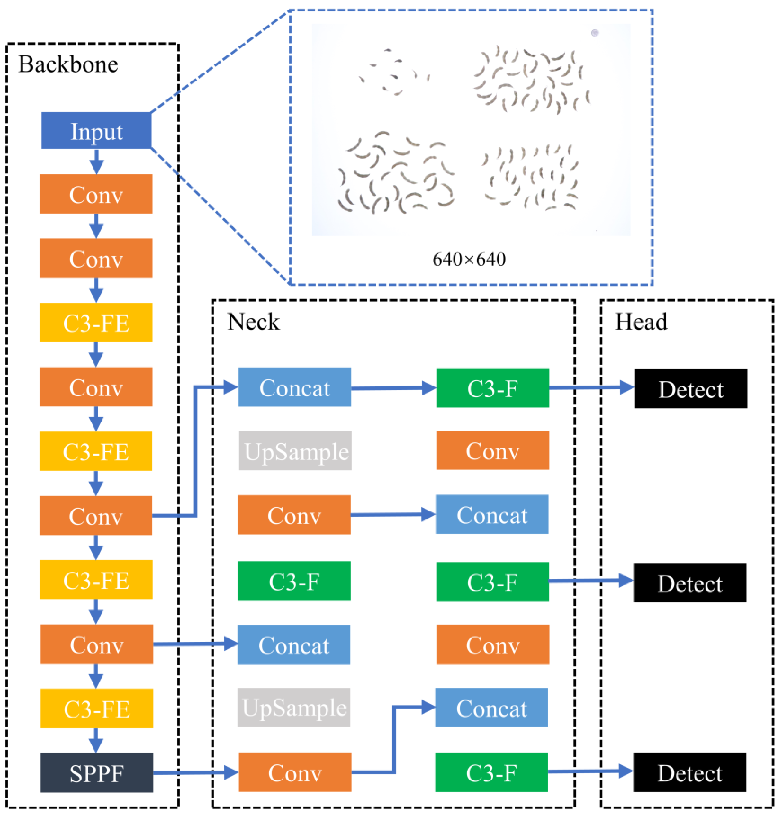
2. Methodology

2.1. FEI-YOLO

The YOLO (You Only Look Once) series models [28] are state-of-the-art models with relatively good performance in general object detection tasks. This series of models uses a regression method for bounding box detection and classification. Among them, the YOLOv5 model performs relatively well and is stable.

Yet it usually needs task-specific adaption to obtain optimal performance. YOLOv5 is mainly divided into four parts: Input, Backbone, Neck, and Head. The Input section standardizes image input sizes and performs data augmentation. The Backbone section discards the Focus structure used in previous series models and employs a traditional 64 × 64 convolutional layer to reduce the number of parameters. Although the Neck layer in YOLOv5 and YOLOv4 both use the Feature Pyramid Network (FPN) [29] and the Path Aggregation Network (PAN) [30], YOLOv5 employs the CSP2 structure based on Cross Stage Partial Networks (CSPNet) [31], which effectively enhances the network’s feature fusion capability. The Head section is used to predict and output the extracted and learned features on the image.

To improve the detection accuracy of pod types and enhance detection speed, this paper proposes to improve the YOLOv5s model from three aspects. Firstly, the C3 modules in the backbone and neck networks are enhanced using the FasterNet structure since they are the most costly and important components. Then, the EMA is incorporated into the C3 modules within the backbone network to optimize the model’s detection performance of the easily confused pod types. Finally, Inner-IoU loss with the CIoU standard loss is carried out to further improve the detection accuracy and generalization of the model. The overall structure of FEI-YOLO is shown in Figure 1.

2.2. Model Lightweighting with FasterNet

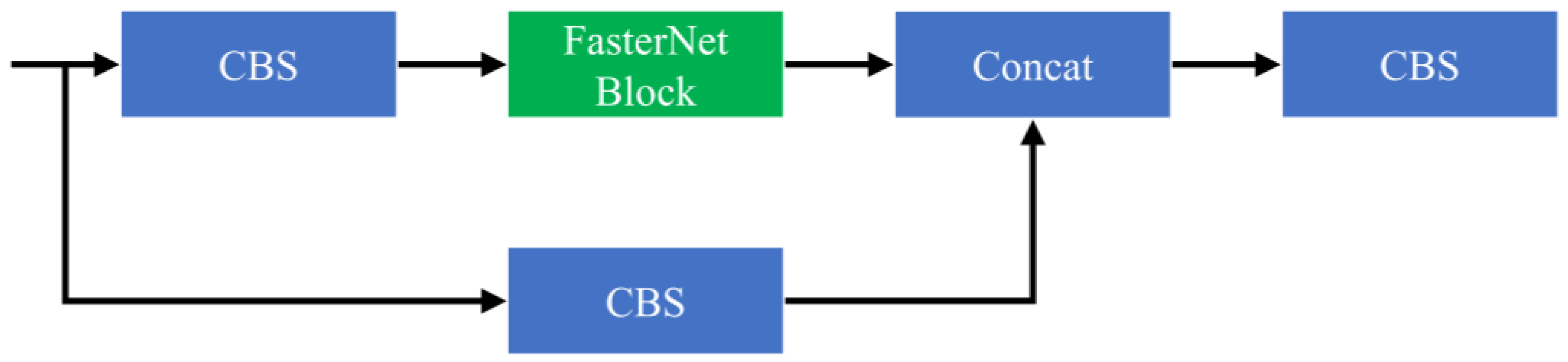
The original C3 module in YOLOv5 contains one or more BottleNeck modules, each comprising a 1 × 1 convolution and a 3 × 3 convolution layer. Although this design enables the C3 module to learn rich feature representations, it also increases the computational load and complexity of the model.

To lightweight the model and enhance detection speed, this paper replaces the BottleNeck modules in the C3 module with the FasterNet Block modules from FasterNet, resulting in the C3-F module, as shown in Figure 1. With this substitution, we significantly reduce the number of parameters and computational load while maintaining the model’s effectiveness in extracting important and representative features, thereby accelerating the inference speed of the original network. The detailed structure of the C3-F module is shown in Figure 2.

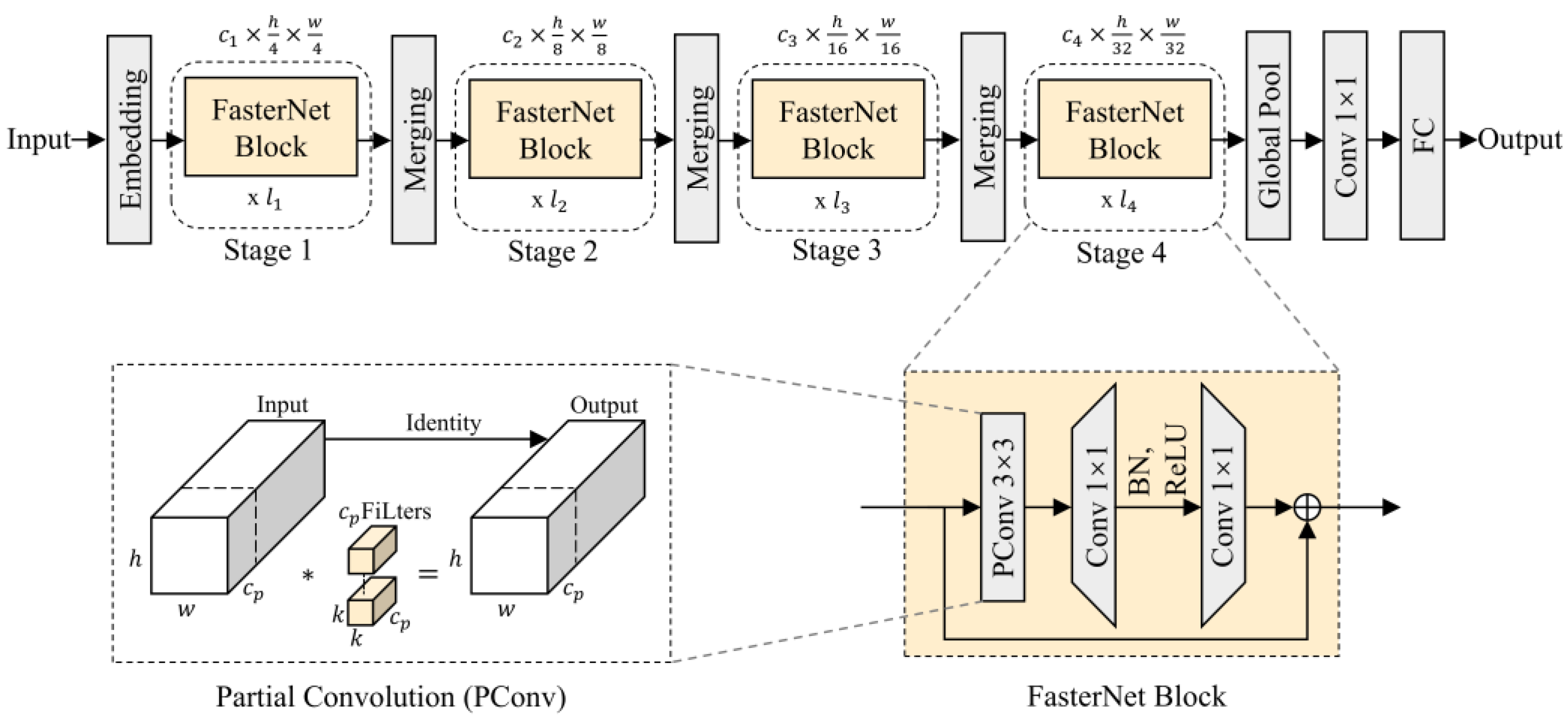
FasterNet [26] is a new neural network structure for visual tasks proposed in 2023. This network structure offers faster operation speed without compromising the accuracy of various tasks. The structure of FasterNet is shown in Figure 3.

The most significant modification introduced by FasterNet is the Partial Convolution (PConv) module, which applies standard convolution to only a proportion of the input channels to extract spatial features, instead of all the channels. PConv is highly parallelizable, allowing all pixels to be processed simultaneously, which enables efficient acceleration on GPUs. By using fewer operations to achieve the same accuracy, it reduces redundant computations and memory access, thereby improving the extraction of target features. For continuous memory access, only the first or last consecutive $c_p$ channels are used to represent the entire feature map. Without loss of generality, we only consider the case where the input and output feature maps have the same number of channels. The floating-point operations (FLOPs) calculation for PConv is shown in Equation (1), and the memory usage calculation is shown in Equation (2), where $h$ and $w$ are the height and width of the feature map, and $k$ is the size of the convolution kernel.

$$h\times w\times k^2\times {c_p}^2$$

(1)

$$h\times w\times 2c_p+k^2\times {c_p}^2\approx h\times w\times 2c_p$$

(2)

When using the common value ${\displaystyle \frac{c_p}{c}}={\displaystyle \frac{1}{4}}$, meaning only 1/4 of the channels undergo partial convolution, the FLOPs of PConv are only 1/16 of those of a standard convolution, and the memory access is 1/4 of that of a standard convolution.

As shown in Figure 3, the FasterNet Block consists of one PConv module and two Pointwise Convolution (PWConv) modules, with normalization layers and activation functions placed between the two PWConv modules to maintain feature diversity and achieve low latency. PWConv is used to restore the number of channels in the feature map and can encode the relationships between channels. This integration of spatial and channel information generated by PConv enhances the network’s expressive capability. Finally, the input feature map is added to the output feature map to obtain the final output result. The PWConv module contains only 1 × 1 convolutional kernels, which changes the number of feature channels without altering the size of the feature map, effectively reducing computational complexity.

2.3. Enhancing Type-Distinctive Representation with EMA

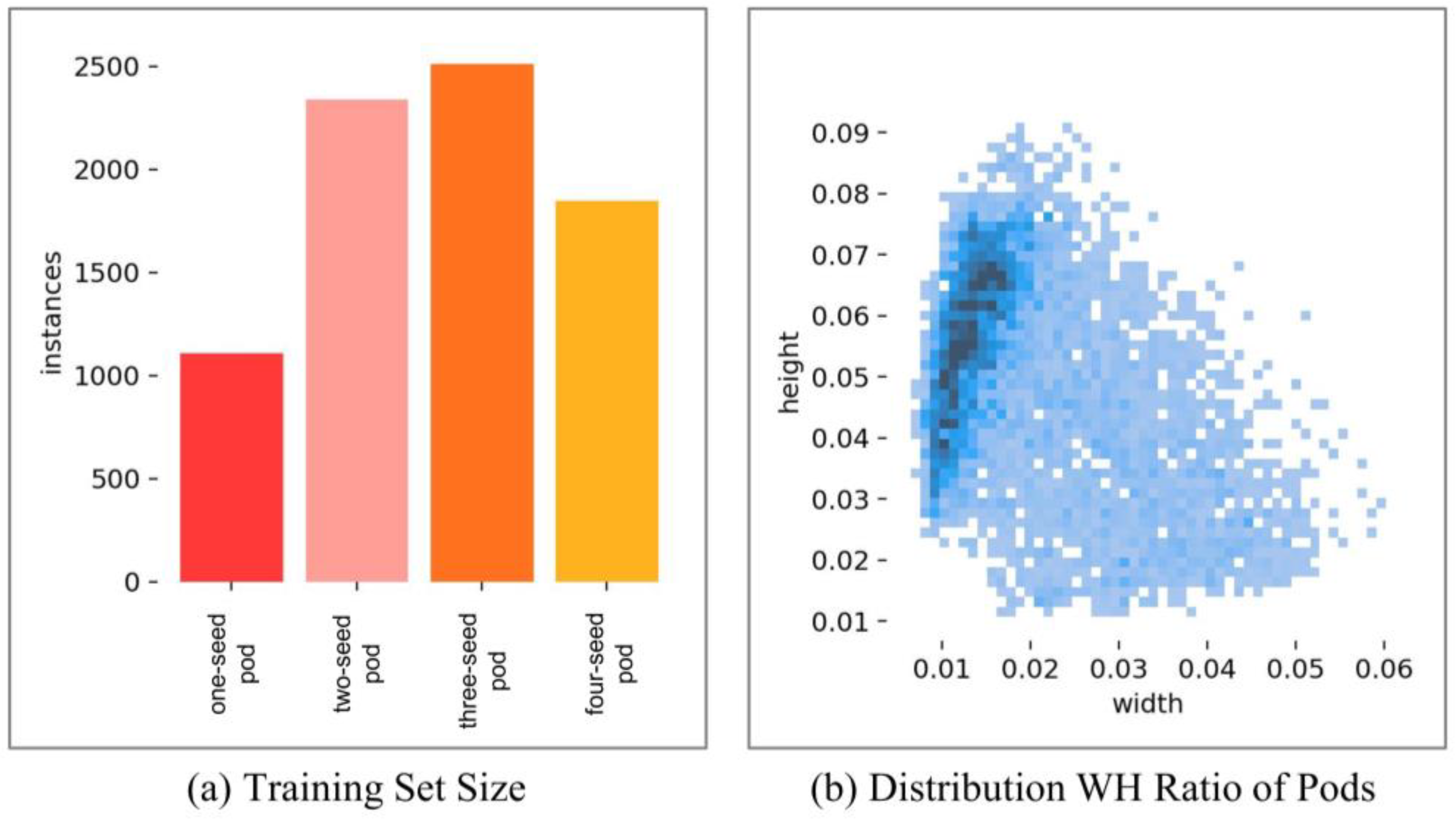
There is a significant difference in the number of pods with various numbers of seeds. Pods with two seeds and three seeds are the majority, yet they are also the most confusing pod types. Moreover, their visual phenotypic features can vary across different soybean plant varieties. The sample distribution of the dataset is shown in Figure 4, where Figure 4a represents the type distribution in the training set, and Figure 4b shows the width-to-height (WH) ratio of the target objects to the entire image.

As shown in Figure 4a, there exists a significant imbalance between different pod types. The number of three-seed pod samples is the highest, approximately 2.5 times the number of one-seed pod samples. As shown in Figure 4b, due to the different pod types, the size of the detection boxes is also unbalanced. Most pods have a width-to-image ratio between 0.01 and 0.02, and a height-to-image ratio between 0.05 and 0.07. However, many pods still have a wide range of width-to-height ratios, which is unfavorable for model training.

Therefore, to adapt to changes in image scale and capture the distinguishing features of different types of pods, this paper introduces the Efficient Multi-Scale Attention (EMA) [25] module. This module ensures the retention of information in each channel without the need for dimensionality reduction and reduces the computational burden. It can reconfigure a portion of the channels into batch dimensions and group them into multiple sub-features, ensuring uniform spatial semantic feature distribution within each feature group. Compared to the alternative Squeeze-and-Excitation (SE), Convolutional Block Attention Module (CBAM), and Coordinate Attention (CA) mechanisms, the EMA module not only offers better performance but is also more efficient in terms of required parameters. This paper incorporates the EMA module into the C3 module of the backbone network, combining it with the previously mentioned C3-F to form C3-FE. The structure is illustrated in Figure 5. This structure retains the advantages of the C3-F module in processing local features while incorporating the strengths of the EMA module in capturing global contextual information. This improvement enhances the model’s ability to focus on target-specific features, enabling it to more accurately extract characteristic information from the target objects in the image.

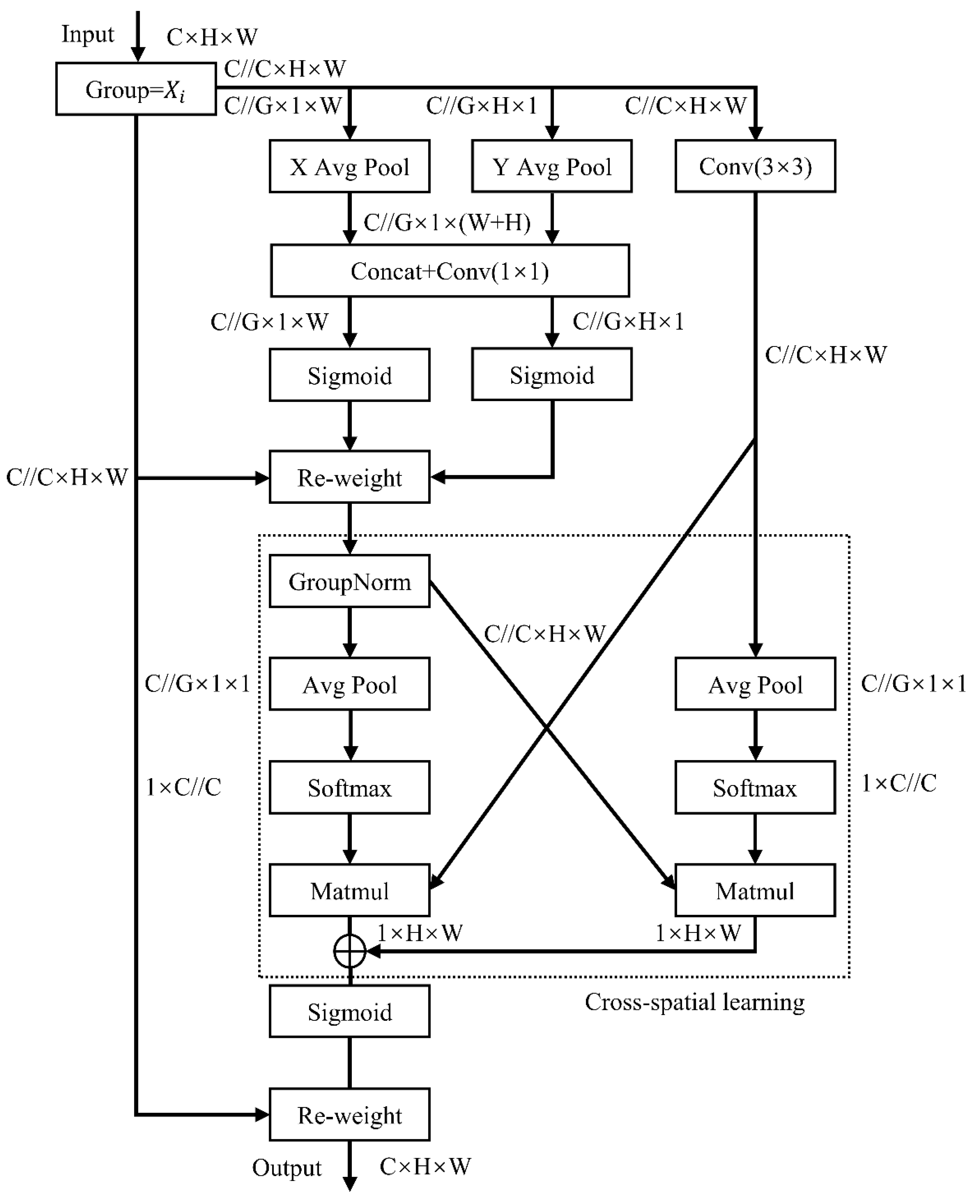
The detailed structure of the EMA module is shown in Figure 6. Let $C$ represents the number of channels, $G$ represents the number of groups, $H$ the height, $W$ the width, ‘$\ll$’ indicates much less than, and ‘$//$’ indicates floor division. For the input feature $X{R}^{C\times H\times W}$, the EMA module first divides it into $G$ sub-features along the channel dimension $X=[X_0,\dots ,X_i,\dots {,X}_{G-1}]$, where $X_i{R}^{C//C\times H\times W}$, with $G\ll C$. Each sub-feature $X_i$ is enhanced through learned attention weights. For each sub-feature, the EMA module extracts the attention weights of the grouped feature maps through three parallel branches. The first two branches include 1 × 1 convolutions and use adaptive global average pooling to encode the channels along the $X$ and $Y$ directions, respectively. The two encoded features are then concatenated, and a shared 1 × 1 convolution is applied, followed by linear fitting using the Sigmoid activation function. The third branch includes a 3 × 3 convolution aimed at capturing multi-scale feature representations. In the cross-spatial learning section, the EMA module aggregates cross-spatial information from different spatial dimensions. First, the global information output by the 1 × 1 branch is normalized. Next, 2D global average pooling is used to encode the global spatial information from both the 1 × 1 and 3 × 3 branches. The Softmax function is then employed to fit a linear transformation, directly converting the channel features of the branch with the smallest output into the corresponding dimensional shape to achieve cross-spatial information aggregation. Finally, the cross-spatial interaction module aggregates the two-channel attention weight values, capturing pixel-level pairwise relationships. The features are output through the Sigmoid activation function, thereby enhancing the original input features and producing the final output feature map.

2.4. Enhancing CIoU with Inner-IoU

Loss function is the guide for a learning model. Models for the target detection typically use the Intersection over Union (IoU) [32] loss function, which is a crucial component of mainstream loss functions. The IoU is defined as follows: $B$ and $B^{gt}$ represent the predicted box and the ground truth (GT) box, respectively.

$$IoU={\displaystyle \frac{\left|B\cap B^{gt}\right|}{\left|B\cup B^{gt}\right|}}$$

(3)

$$L_{IoU}=1-IoU$$

(4)

The bounding box regression loss function family based on the IoU have continuously evolved, including variants such as the Generalized IoU (GIoU), Distance IoU (DIoU), Complete IoU (CIoU), Extended IoU (EIoU), and Scalable IoU (SIoU).

The default loss function used by YOLOv5 is the CIoU, a loss function commonly used in classification problems [33]. It measures the accuracy of object detection models in terms of detecting the position and size of the target, effectively handling the overlap and misalignment between bounding boxes, thereby improving the performance evaluation of the model.

The CIoU is defined as follows: Let $b$ and $b^{gt}$ represent the predicted box and the GT box, respectively. ${\displaystyle \frac{{\rho }^2\left(b,b^{gt}\right)}{C^2}}$ represents the distance between their center points. The greater the distance, the higher the penalty. This mechanism ensures that the predicted box not only overlaps in area but is also positioned closer to the ground truth box. The term $av$ represents the aspect ratio consistency penalty mechanism. The greater the difference, the higher the penalty. This mechanism ensures that the predicted box matches the shape of the ground truth box as closely as possible. $v$ includes the aspect ratio to be predicted, and $a$ is a positive weighting parameter. $w^{gt}$ and $h^{gt}$ denote the width and height of the ground truth box, while $w$ and $h$ denote the width and height of the predicted box.

$$L_{CIoU}=1-IoU+{\displaystyle \frac{{\rho }^2\left(b,b^{gt}\right)}{C^2}}+av$$

(5)

$$v={\displaystyle \frac{4}{{\pi }^2}}{(arctan{\displaystyle \frac{w^{gt}}{h^{gt}}}-arctan{\displaystyle \frac{w}{h}})}^2$$

(6)

$$a={\displaystyle \frac{v}{\left(1-IoU\right)+v}}$$

(7)

The CIoU has certain limitations. On one hand, it has a weaker ability to evaluate objects with large aspect ratios and irregular shapes. On the other hand, it cannot adaptively adjust to various detection tasks and targets, and it does not account for the balance between different samples. When there is substantial variability among samples, it can also constrain the convergence speed of the model [32,34].

In this dataset, the $w$ and $h$ of the pods are relatively small with significant ratio differences, which increases the aspect ratio consistency penalty term in the CIoU, thereby reducing the CIoU value. This causes the CIoU to fail to reflect the real situation and may optimize similarity in an unreasonable way. To address these limitations, this paper introduces the Inner-IoU [27] loss function based on auxiliary bounding boxes. The Inner-IoU is a more detailed and target-center-focused performance evaluation metric. By using the scale of auxiliary bounding boxes, it enhances the accuracy and efficiency of object detection tasks, aligning well with practical needs. In the Inner-IoU, the scale factor ratio is introduced to control the size of the auxiliary bounding boxes. Calculating the IoU using smaller-scale auxiliary bounding boxes aids in the regression of high-IoU samples, accelerating convergence. Using larger-scale auxiliary bounding boxes for IoU loss calculation speeds up the regression process of low-IoU samples. Employing auxiliary bounding boxes of different scales for different datasets and detectors overcomes the limitations of existing methods in terms of generalization capability.

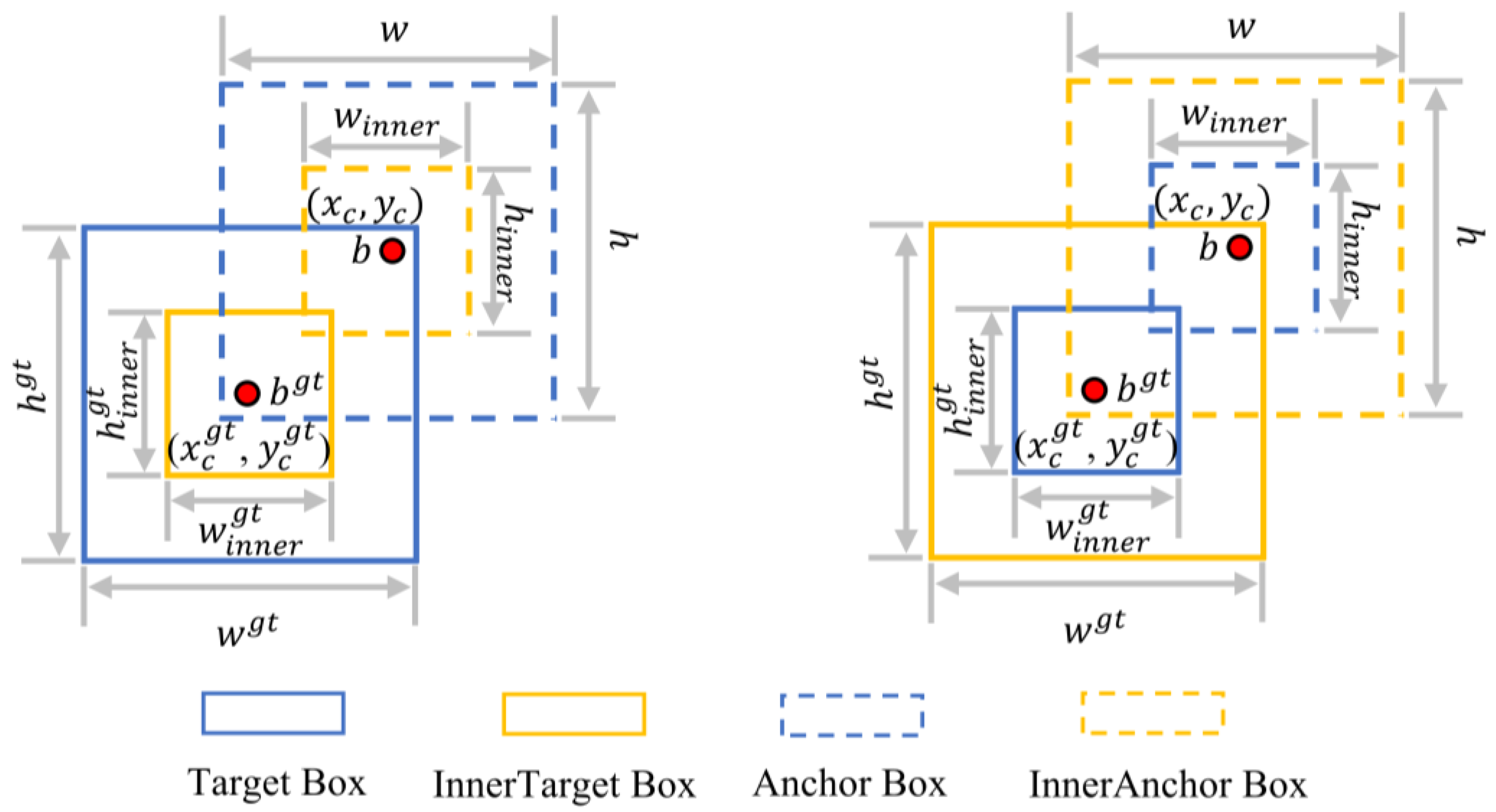
The Inner-IoU is defined as follows: $b$ and $b^{gt}$ represent the predicted box and the GT box, respectively, as illustrated in Figure 7. $w$ and $h$ are the width and height of the predicted box, and $w^{gt}$ and $h^{gt}$ are the width and height of the GT box, respectively. ${(x}_c,y_c)$ represents the center point of the predicted box, and $(x_c^{gt},y_c^{gt})$ represents the center point of the GT box. The variable ratio corresponds to the scale factor, typically ranging from [0.5, 1.5].

$$b_l^{gt}=x_c^{gt}-{\displaystyle \frac{x_c^{gt}\times radio}{2}},b_r^{gt}=x_c^{gt}+{\displaystyle \frac{w^{gt}\times radio}{2}}$$

(8)

$$b_t^{gt}=y_c^{gt}-{\displaystyle \frac{h_c^{gt}\times radio}{2}},b_b^{gt}=y_c^{gt}+{\displaystyle \frac{h^{gt}\times radio}{2}}$$

(9)

$$b_l=x_c-{\displaystyle \frac{w\times radio}{2}},b_r=x_c+{\displaystyle \frac{w\times radio}{2}}$$

(10)

$$b_t=y_c-{\displaystyle \frac{h\times radio}{2}},b_b=y_c+{\displaystyle \frac{h\times radio}{2}}$$

(11)

$$inter=\left(\min \left(b_r^{gt},b_r\right)-\max \left(b_l^{gt},b_l\right)\right)\times \left(\min \left(b_b^{gt},b_b\right)-\max \left(b_t^{gt},b_t\right)\right)$$

(12)

$$union=\left(w^{gt}\times h^{gt}\right)\times {\left(radio\right)}^2+\left(w\times h\right)\times {\left(radio\right)}^2-inter$$

(13)

$${IoU}^{inner}={\displaystyle \frac{inter}{union}}$$

(14)

$$L_{Inner-CIoU}=L_{CIoU}+IoU-{IoU}^{inner}$$

(15)

This paper applies the Inner-IoU to the CIoU, resulting in the loss function Inner-CIoU. This loss function not only retains the advantages of the CIoU but also controls the size of the auxiliary bounding boxes through the scale factor ratio, enhancing the model’s generalization ability. By allowing the model to focus more on the target center, it effectively mitigates the issue of the CIoU value reduction due to significant aspect ratio differences in pods, thereby improving detection accuracy.

2.5. Dataset

The soybean plant samples used in this study were obtained from the experimental field of the College of Agriculture at Yangtze University. The plants were planted in June 2023 and harvested in October 2023, with a maturity period of 82 to 126 days.

To obtain the characteristic information of soybean pods, the LabelImg data annotation tool was used to label the pods in each image. Pods were categorized as one-seed pods, two-seed pods, three-seed pods, and four-seed pods according to the number of seeds they have. An example from each pod type is shown in Figure 8. The collected data were then randomly divided into training, validation, and test sets in a 7:2:1 ratio. The number of targets for each label is shown in

Table 1. Distribution of the subsets and pod types.

Dataset	One-Seed Pod	Two-Seed Pod	Three-Seed Pod	Four-Seed Pod
Train	1103	2337	2512	1844
Val	351	694	720	469
Test	117	316	335	278
Total	1571	3347	3567	2591

. There are a total of 11,076 pod targets. Two-seed pods and three-seed pods are the majority, with 3347 and 3567 targets, respectively. This is followed by the four-seed pod type with 2591 targets. The one-seed pod type has the fewest targets, with 1571 targets.

2.6. Experimental Setup

All experiments in this paper were conducted on the same platform. The operating system was Windows 10, with Python 3.9, PyTorch 2.0.1, CUDA 11.8, an Intel i5-12600KF CPU, an NVIDIA RTX 3090Ti GPU, and 32 GB of memory. Both the original and improved models used the same hyperparameters, as shown in

Table 2. Experimental hyperparameter setting.

Epochs	Batch-Size	Workers	Imgsize	Optimizer	Momentum	Lr0	Ratio
500	8	8	640	SGD	0.937	0.01	0.75

. The hyperparameters of this experiment are all set by default.

2.7. Performance Indicator

To evaluate the stability and recognition performance of the network model, this study employs classic object detection performance metrics, including Precision ($P$), Recall ($R$), and mean Average Precision ($mAP$).

$$P={\displaystyle \frac{TP}{TP+FP}}$$

(16)

$$R={\displaystyle \frac{TP}{TP+FN}}$$

(17)

$$AP=\sum _{i=1}^{N}P\left(i\right)∆R\left(i\right)$$

(18)

$$mAP={\displaystyle \frac{{\sum }_{i=1}^{k}A{P}_i}{k}}$$

(19)

Positive samples: pod types correctly identified by the model; negative samples: pod types incorrectly identified by the model. True Positives ($TP$): correctly identified as positive samples. True Negatives ($TN$): correctly identified as negative samples. False Positives ($FP$): incorrectly identified as positive samples. False Negatives ($FN$): incorrectly identified as negative samples. $N$ represents the number of images, $AP$ represents the average precision for the current type, and $k$ denotes the number of types in the detection task.

3. Results and Analysis

3.1. Baseline Model Prior Experiments

To explore the best baseline model, this paper evaluates the performance of three versions of the YOLOv5 baseline model. In the metrics presented in

Table 3. Baseline model prior experiments.

Model	$\mathit{m}\mathit{A}\mathit{P}\mathbf{@}\mathbf{0.5}$/%	$\mathit{m}\mathit{A}\mathit{P}\mathbf{@}\mathbf{[}\mathbf{0.5}\mathbf{:}\mathbf{0.95}\mathbf{]}$/%	FLOPs/G	Params/M	FPS
YOLOv5n	96.1	75.8	7.2	2.45	152
YOLOv5s	97.1	79.7	24.0	8.91	103
YOLOv5m	97.2	79.9	64.4	24.5	78

, floating-point operations (FLOPs) and the number of parameters (Params) are evaluation standards for lightweight models. FLOPs represent the number of floating-point operations required for a model to perform inference, reflecting the model’s computational complexity. Lower FLOPs indicate faster inference speeds. Params is a key metric for evaluating the model’s size; lower Params indicate that the model requires less memory space. Frames per second (FPS) is used to evaluate model speed. Higher FPS indicates a faster detection rate.

The experimental results indicate that, although the YOLOv5n model has the smallest computational load and the fastest detection speed, its average detection accuracy is considerably lower. While the YOLOv5m model shows some improvement in average detection accuracy, it has a significantly higher computational load and slower detection speed compared to the YOLOv5n and YOLOv5s models. Balancing these factors, the YOLOv5s model, despite sacrificing some detection speed, can largely maintain a high detection accuracy. Therefore, this paper adopts the YOLOv5s model as the baseline model.

3.2. Model Comparison Experiment

To further verify the detection performance of FEI-YOLO, it was compared with current mainstream object detection models, including SSD, Faster RCNN, YOLOv3, YOLOv5s, YOLOv7, YOLOv8s, YOLOv9s and YOLOv10s. The detection results of each model are shown in

Table 4. Performance comparison of different models.

Model	$\mathit{m}\mathit{A}\mathit{P}\mathbf{@}\mathbf{0.5}$/%	$\mathit{m}\mathit{A}\mathit{P}\mathbf{@}\mathbf{[}\mathbf{0.5}\mathbf{:}\mathbf{0.95}\mathbf{]}$/%	FLOPs/G	Params/M	FPS
SSD	14.8	3.3	62.7	26.29	71
Faster RCNN	15.2	4.3	370.2	137.09	34
YOLOv3	87.9	54.7	12.9	8.48	145
YOLOv5s	97.1	79.7	24.0	8.91	103
YOLOv7	97.4	76.8	105.2	36.33	84
YOLOv8s	96.9	78.2	28.4	10.6	98
YOLOv9s	97.2	79.5	39.6	9.29	92
YOLOv10s	92.7	77.3	24.8	8.69	106
FEI-YOLO	98.6	81.1	21.4	7.73	127

.

As shown in the table, FEI-YOLO has significant advantages in detection accuracy and Params. Its $mAP@0.5$ and $mAP@\left[0.5;0.95\right]$ are 98.6% and 81.1%, respectively, the highest among all models, and its Params is 7.73 M, the smallest among all models. The FLOPs of FEI-YOLO is 21.4 G, which is slightly higher than YOLOv3’s 12.9 G but lower than the FLOPs of all other models. Its FPS reaches 127, second only to YOLOv3. Despite slightly higher FLOPs and lower FPS compared to YOLOv3, FEI-YOLO significantly outperforms it in detection accuracy. These results indicate that, compared to mainstream object detection models, FEI-YOLO can maintain detection accuracy while achieving model lightweighting. YOLOv7’s $mAP@0.5$ is 0.3% higher than YOLOv5s, but its FLOPs and Params are 4.4 times and 4.1 times those of YOLOv5s, respectively. This poses challenges for fast image processing and model deployment. Experiments show that YOLOv8s performs worse than YOLOv5s in both $mAP@0.5$ and $mAP@\left[0.5;0.95\right]$, while its FLOPs and parameters are larger, and FPS is lower, making it a less favorable option. Although YOLOv9s is comparable to YOLOv5s in both $mAP@0.5$ and $mAP@\left[0.5;0.95\right]$; its FLOPs are 1.7 times higher, and it falls short in terms of parameters and FPS. As for YOLOv10s, it offers no advantage in detection accuracy compared to other models in the YOLO series, so it is not considered further. This paper chooses YOLOv5s as the baseline model, ensuring detection accuracy, achieving model lightweighting, and maintaining processing speed.

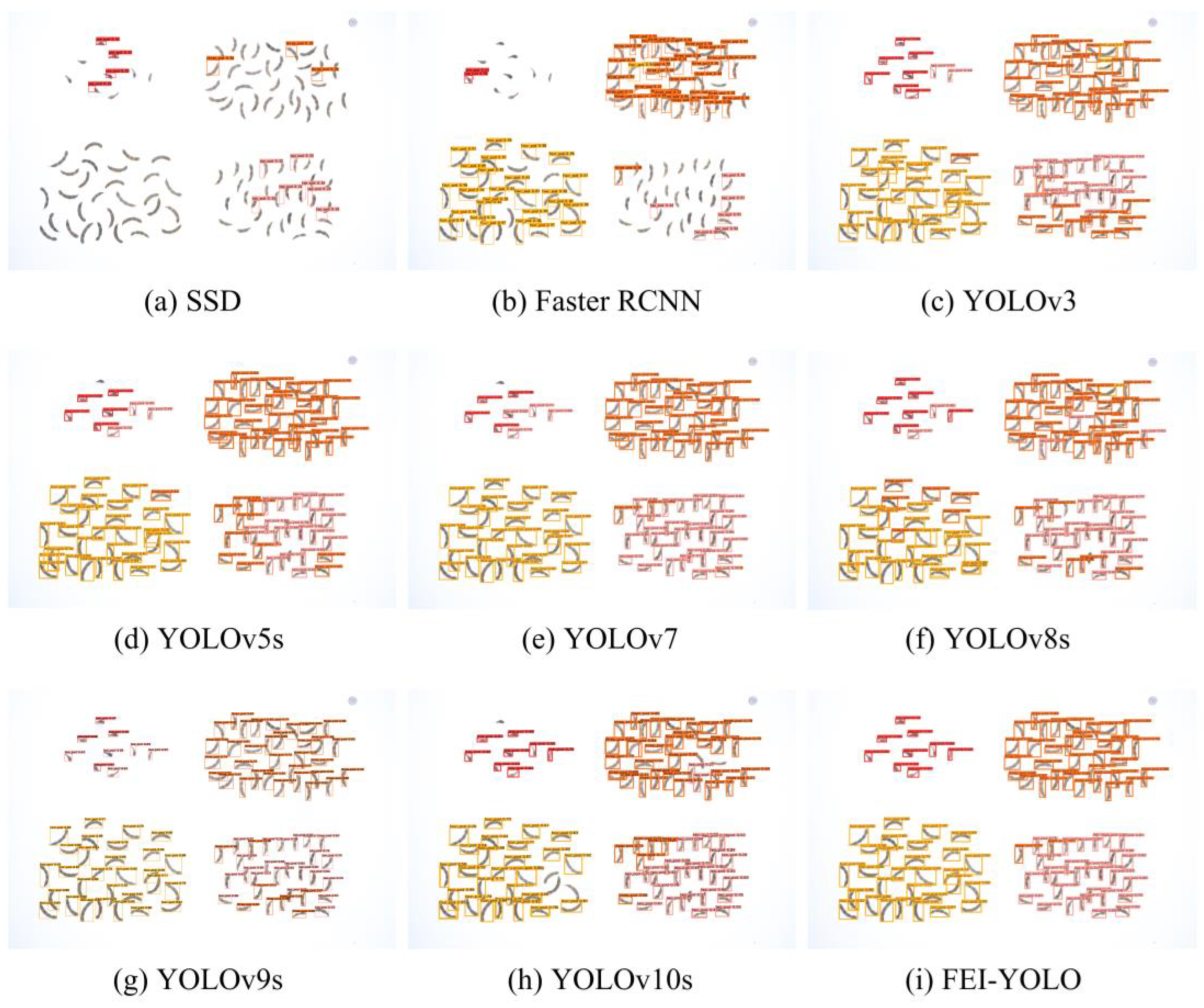
To intuitively display the detection performance of each model, Figure 9 compares the detection results of various models on the same image. As shown in the figure, SSD has the worst detection performance, with a high miss detection rate for all pod types. This indicates that the SSD model may not have learned the corresponding features. Faster RCNN shows a significant improvement in detecting three-seed pod and four-seed pod types, but it remains insensitive to one-seed pod and two-seed pod features, failing to achieve a higher accuracy over all pod types. Although YOLOv3 can detect all types of pods, it has a relatively high error rate in classification, particularly for the two-seed pod type. YOLOv5s performs relatively well in terms of recognition, but there are some errors in one-seed pod and two-seed pod types. YOLOv7 and YOLOv9s have detection errors for one-seed pod types, with YOLOv9s also showing errors in the two-seed pod type. YOLOv8s and YOLOv10s exhibit errors in the detection of two-seed, three-seed, and four-seed pod types. Compared to the aforementioned YOLO series models, FEI-YOLO can accurately detect all pods in the one-seed pod type and shows significant improvement in the misdetection of two-seed pod and three-seed pod types.

The prediction results of a model are the most intuitive way to evaluate its performance.

Table 5. Comparison of $TP$, $FP$, and $FN$ counts for different models on the same image.

Model	One-Seed Pod			Two-Seed Pod			Three-Seed Pod			Four-Seed Pod
	$TP$	$FP$	$FN$	$TP$	$FP$	$FN$	$TP$	$FP$	$FN$	$TP$	$FP$	$FN$
SSD	4	0	5	2	5	26	3	0	32	0	0	29
Faster RCNN	1	1	8	5	1	23	19	14	16	24	1	5
YOLOv3	7	0	2	19	5	9	30	15	5	27	6	2
YOLOv5s	5	0	4	20	4	8	33	12	2	28	2	1
YOLOv7	4	0	5	27	2	1	33	4	2	28	1	1
YOLOv8s	7	0	2	22	6	6	32	14	3	24	3	5
YOLOv9s	4	0	5	21	6	7	33	8	2	28	1	1
YOLOv10s	8	0	1	22	3	6	29	10	6	25	4	4
FEI-YOLO	9	0	0	27	1	1	33	2	2	28	2	1

quantifies the detection results shown in Figure 9 by comparing the corresponding number of $TP$, $FP$, and $FN$ for different models. This comparison provides an instance of the predictive performance of each model based on the counts of $TP$, $FP$, and $FN$.

Table 6. Comparison of FEI-YOLO and YOLOv5s performance on different pod types.

Model	$\mathit{A}\mathit{P}$/%				$\mathit{m}\mathit{A}\mathit{P}\mathbf{@}\mathbf{0.5}$/%	$\mathit{m}\mathit{A}\mathit{P}\mathbf{@}\mathbf{[}\mathbf{0.5}\mathbf{:}\mathbf{0.95}\mathbf{]}$/%
	One-Seed Pod	Two-Seed Pod	Three-Seed Pod	Four-Seed Pod
YOLOv5s	97.7	97.1	96.0	97.5	97.1	79.7
FEI-YOLO	98.8	98.6	98.3	98.6	98.6	81.1

compares the recognition performance of FEI-YOLO and YOLOv5s across different pod types. Compared to YOLOv5s, FEI-YOLO’s AP was improved by 1.1%, 1.5%, 2.3%, and 1.2% for one-seed pod, two-seed pod, three-seed pod, and four-seed pod types, respectively. Overall, the accuracy of all types was improved after the modifications. The most significant improvement was observed in the three-seed pod type, followed the by two-seed pod type. The reason for this is that these two types are easily confused. The inclusion of the EMA module in FEI-YOLO enhances the model’s ability to extract features from target regions more accurately. This leads to better feature acquisition of the targets to be detected, resulting in improved accuracy for smaller targets like the one-seed pod. Additionally, it becomes easier to distinguish between the easily confused two-seed pod and three-seed pod types, thereby improving the overall detection accuracy.

3.3. Ablation Experiment

To verify the effectiveness of the improvements made to the FEI-YOLO modules, ablation experiments were conducted using the YOLOv5s model as the baseline. The specific results are shown in

Table 7. Ablation experiment results.

Model	$\mathit{m}\mathit{A}\mathit{P}\mathbf{@}\mathbf{0.5}$/%	$\mathit{m}\mathit{A}\mathit{P}\mathbf{@}\mathbf{[}\mathbf{0.5}\mathbf{:}\mathbf{0.95}\mathbf{]}$/%	FLOPs/G	Params/M	FPS
YOLOv5s	97.1	79.7	24.0	8.91	101
YOLOv5s + InnerIOU	97.7	80.3	24.0	8.91	104
YOLOv5s + FasterNet	97.4	80.1	20.9	7.71	138
YOLOv5s + FasterNet + InnerIOU	98.1	80.5	20.9	7.71	140
YOLOv5s + FasterNet + EMA	98.2	80.8	21.4	7.73	125
FEI-YOLO	98.6	81.1	21.4	7.73	127

.

The data in the table lead to the following conclusions: In the ablation experiments of individual modules, replacing the CIoU with Inner-IoU improved the model’s detection accuracy, with both $mAP@0.5$ and $mAP@[0.5:0.95]$ increasing by 0.6%. By improving the YOLOv5s model’s C3 module with FasterNet, specifically using the C3-F module, the model’s FLOPs were reduced by 13% and Params by 13.5%, indicating a significant lightweighting effect. Meanwhile, $mAP@0.5$ increased by 0.3% and $mAP@[0.5:0.95]$ increased by 0.4%, ensuring the detection accuracy of the model. The improvement of the EMA module is based on the FasterNet-enhanced C3 module. After further enhancing the C3-F module in the backbone network with the EMA module, the model’s FLOPs and Params increased slightly, but $mAP@0.5$ improved by 0.8%, $mAP@[0.5:0.95]$ and improved by 0.7%, showing a clear improvement. On the premise of using the C3-F module, replacing CIoU with Inner-IoU resulted in an increase of 0.7% in $mAP@0.5$ and a 0.4% increase in $mAP@[0.5:0.95]$.

The ablation experiments show that all three improvement methods are effective, each providing a certain degree of enhancement compared to the baseline YOLOv5s model. The FEI-YOLO model, compared to the YOLOv5s algorithm, achieves a 10.8% reduction in FLOPs, a 13.2% reduction in Params, a 1.5% increase in $mAP@0.5$, a 1.4% increase in $mAP@[0.5:0.95]$, and a 25.7% elevation in FPS, making it the optimal solution for both lightweighting and detection accuracy.

To comprehensively study the performance of FEI-YOLO, Figure 10 shows the performance differences between FEI-YOLO and YOLOv5s under the same parameter settings. As shown in Figure 10a, compared to YOLOv5s, FEI-YOLO not only has an improvement in detection accuracy but also converges faster. The $mAP@0.5$ value of YOLOv5s stabilizes around 450 iterations, whereas the accuracy of FEI-YOLO stabilizes significantly before 400 iterations. The comparison in Figure 10b between FEI-YOLO and YOLOv5s in terms of $mAP@[0.5:0.95]$ further demonstrates that FEI-YOLO achieves higher detection accuracy and faster convergence.

4. Discussion

The following will discuss the FEI-YOLO model from three aspects: its innovation and modification compared with the benchmark model, its comparison with related research, and its potential as an automated tool for agricultural research and production.

1.

All the improvements upon the standard YOLO model proposed in this article focus on lightweighting the model and improving detection accuracy on easily confused pod types, and the experimental results show that all the improvements are effective. By replacing the Bottleneck component in the C3 module of the benchmark model with the FasterNet Block in FasterNet, the proposed FEI-YOLO model successfully reduces the FLOPs of the model by 12.9% and the number of parameters by 13.5%. The FEI-YOLO model is effectively lightweight. At the same time, $mAP@0.5$ and $mAP@[0.5:0.95]$ are increased by 0.3% and 0.4% respectively, ensuring the detection accuracy of the lightweight model. Furthermore, the EMA attention mechanism is integrated into the backbone network to enhance the model’s focus on target features, particularly on the easily confused pod types. With this enhancement, the FEI-YOLO model’s $mAP@0.5$ and $mAP@0.5$ values are increased by 0.8% and 0.5%, significantly improving detection accuracy. Last but not least, the Inner-IoU loss function was used to improve the CIoU loss function, the model’s $mAP@0.5$ and $mAP@[0.5:0.95]$ values both increased by 0.6% as compared with the benchmark model YOLOv5s.

2.

The proposed FEI-YOLO model’s detection accuracy surpasses counterpart models in related work. For example, Lu et al. [18] achieved a detection accuracy of 90.3% for pod types using an improved YOLOv3 model, while Uzal et al. [19] attained 86.2% accuracy with a CNN-based model. In contrast, the FEI-YOLO model demonstrated a significantly higher accuracy of 98.6%, showcasing superior detection performance. Another feature of the FEI-YOLO model is that it can directly process multiple pods within a single image, without requiring the image to be cropped into fragments of individual pod images first [20]. For the easily confusing two-seed and three-seed pod types, Yan et al. [20] achieved accuracies of 95.8% and 95.6%, respectively, using images that each contain only one single pod. In contrast, the FEI-YOLO model obtained $AP$ scores of 98.6% on two-seed pods and 98.3% on three-seed pods, demonstrating its enhanced capability in detecting these challenging cases. These comparisons indicate that the FEI-YOLO model is more flexible with input images and is more effective at identifying easily confusing pod types.

3.

Based on the above analysis, the proposed FEI-YOLO model can serve as an efficient tool for agricultural researchers, offering valuable insights into soybean seed selection and other crop performance analyses and contributing to the automation and digitization of agricultural research and production.

5. Conclusions

This paper proposes the FEI-YOLO model based on soybean pod-type detection. By integrating FasterNet into the backbone and neck networks, the model achieves lightweighting by reducing the number of parameters while maintaining accuracy, thereby addressing the issue of slow detection speed. The incorporation of the EMA module into the backbone network enhances the model’s feature extraction capability, allowing it to more accurately identify pods with similar features. This solves the problem of confusion between two-seed pods and three-seed pods and improves the overall detection accuracy. Additionally, the loss function is replaced with the Inner-IoU, which accelerates the regression of bounding boxes using auxiliary boxes, leading to better convergence. This further enhances the model’s detection accuracy and generalization capability. Based on the analysis of the experimental results, the following conclusions can be drawn:

1.

Model Detection Accuracy: FEI-YOLO achieved $mAP@0.5$ and $mAP@[0.5:0.95]$ scores of 98.6% and 81.1%, respectively, which are the highest scores among all compared models. Compared to the baseline YOLOv5s model, FEI-YOLO’s detection accuracy obtained 1.5% and 1.4% increases, respectively. These results indicate that FEI-YOLO can infer more accurately than the baseline YOLOv5s model.

2.

Model Size and Detection Speed: While improving detection accuracy, FEI-YOLO successfully reduced the model size of the YOLOv5s, reducing the number of parameters by 13.2%. Meanwhile, FEI-YOLO also improved the detection speed, reducing FLOPs by 10.8% and increasing FPS by 25.7%. These results indicate that FEI-YOLO can infer faster and is a more lightweight model than the baseline YOLOv5s model.

Future work will focus on further enhancing the model’s generalization capability to ensure reliable performance across diverse environmental and background conditions, making it more applicable in real-world agricultural scenarios. However, challenges remain, such as difficulties in accurately detecting pods in complex situations, like occlusion or overlap. Future efforts will aim to improve the model’s robustness in these challenging conditions.