Abstract
Reference evapotranspiration (ET0) is one important agrometeorological parameter for hydrological studies and climate risk zoning. ET0 calculation by the FAO Penman–Monteith method requires several input data. However, the availability of climate data has been a problem in many places around the world, so the study of scenarios with different combinations of climate data has become essential. The aim of this study was to evaluate the performance of artificial neural network (ANN), random forest (RF), support vector machine (SVM), and multiple linear regression (MLR) approaches to estimate monthly mean ET0 with different input data combinations and scenarios. Three scenarios were evaluated: at the state level, where all climatological stations were used (Scenario I–SI), and at the regional level, where the Minas Gerais state was divided according to the climatic classifications of Thornthwaite (Scenario II–SII) and Köppen (Scenario III–SIII). ANN and RF performed better in ET0 estimation among the models evaluated in the SI, SII, and SIII scenarios with the following data combinations: (i) latitude, longitude, altitude, month, mean, maximum and minimum temperature, and relative humidity and (ii) latitude, longitude, altitude, month, mean temperature, and relative humidity. SVM and MLR models are recommended for all scenarios in situations with limited climatic data where only air temperature and relative humidity data are available. The results and information presented in this study are important for the agricultural chain and water resources in Minas Gerais state.
1. Introduction
Evapotranspiration is essential information in agriculture. The agriculture sector is found to be a major water consumer in most countries. The proportion of water withdrawn for agriculture in developing counties is estimated at nearly 81%, while it accounts for 71% of water withdrawal globally. Information on evapotranspiration is important in order to estimate crop water requirements and irrigation water requirements and control several hydrological processes [1,2,3]. Evapotranspiration (ET) is an agrometeorological parameter that can be measured using a lysimeter or water balance approach. These methods for measuring ET are not always possible to use. The lysimeter and water balance approaches are time-consuming methods and need precisely and carefully planned experiments [4]. Therefore, the use of evapotranspiration estimation methods is very important, and, for that, an adequate meteorological database is necessary to achieve good estimates [5,6].
The concept of evapotranspiration is related to the transfer rate of water from the soil–plant system to the atmosphere. In this study, we focus on the use of reference evapotranspiration (ET0), which is related to the rate of water consumption from a reference crop surface (grass or alfafa). ET0 can be used for a large area, e.g., for climatic classification of a region [7,8], or for small areas, e.g., for obtaining crop water requirements or crop evapotranspiration (ETc) [9,10,11]. The standard model used today for reference evapotranspiration estimation is the Penman–Monteith evapotranspiration model. This model is considered more realistic physically, but it requires some additional meteorological variables when compared with other methods [8]. This dependence on several meteorological variables combined with the limitations of weather station networks and interruptions and errors in weather databases makes it difficult to measure ET0. Thus, some models are used to estimate ET0. These models seek less dependence on many weather inputs and high predictive power.
Among the models used in the literature, this study focused on the following models: artificial neural network (ANN), random forest (RF), support vector machine (SVM), and multiple linear regression (MLR) models. These models show different levels of predictive capacity for different meteorological variables and in other fields of science [11,12,13,14]. ANN, RF, and SVM models can capture complex relationships between input and output data, which makes them powerful models for modeling. These machine-learning models have been successfully used to estimate ET0 with fewer input meteorological data [12,15,16]. Although the inability of MLR to handle non-linear relationships between dependent and independent variables is evident in some studies, MLR has been successfully used to estimate ET0 [13,17].
Considering the models, ANN is a promising and effective tool for non-linear modeling and complex time series. An ANN’s architecture is composed of three layers—input, hidden, and output layers—and each layer includes an array of processing elements [6,12,16]. Several papers have shown the excellent predictive capacity of ANN models with different architectures in studies with ET0 [14,15,18]. The RF model is a non-parametric statistical data modeling method that is decision-tree-based. RF is a classification and regression technique that has also been adopted to predict agrometeorological parameters such as ET0 [15,19,20]. RF has been found to be a more efficient predicting tool compared with other tools like ANN [11,21]. SVM is a supervised machine-learning algorithm developed by [22]. SVM is used for regression, classification, pattern recognition, and forecasting. This model has been used in meteorological variable estimation and shown high predictive power [23,24]. MLR aims at explaining the collinearity between a dependent variable and an independent variable by means of a linear combination of independent predictor variables (more than one). This regression technique has been adopted in several fields of science, including climatology, hydrology, and irrigation, with varying performance [17].
There is so much literature on evapotranspiration that in this context it is practically impossible to propose even a partial review. Some remarkable recent contributions are due to [25,26,27,28,29,30,31,32]. This paper focuses on ET0 estimation in the Minas Gerais state, Brazil, using different models. Agriculture has an important role in this region and ET0 estimation on a monthly scale is extremely important for the agricultural chain. Among its main applications are the following: (i) climatic classification of a region—fundamental in the zoning of climatic risk in agricultural regions; (ii) hydrological processes—knowledge of evapotranspiration is fundamental in the hydrological cycle and, consequently, all studies related to hydrology and water resources; (iii) crop water requirements or crop evapotranspiration (ETc)—essential information in planning and implementing irrigation projects (i.e., determining the water demand of a given crop during the months of the year); and (iv) agrometeorological modeling—several models use ET data as an input variable for estimating productivity and other important variables; among other applications. This study also presents a relevant and innovative contribution through evaluation of the evapotranspiration estimates considering different climatic scenarios for the same state; that is, for regions which cover an extremely large area (such as the Minas Gerais state), there may be a trade-off between generalization capacity and the performance of developed models. Therefore, data partition in the spatial sense aims to achieve the highest efficiency for the evaluated models, thus becomes relevant for the study of different climatic scenarios.
Considering that the presence of gaps or discontinuities in the meteorological data series can delay the state of development, this study proposes to analyze the use of different combinations of input data and climate scenarios for the accurate estimation of ET0, and, especially, with the minimum possible use of input data in these models, this can facilitate the estimation of ET0. The hypothesis of this study is that models based on machine learning are an efficient tool for estimating evapotranspiration, even under conditions of limited climatic data.
ET0 calculated by the FAO Penman–Monteith method requires several input data. This amount of input data makes it difficult to use this method. New technologies can make it easier to obtain ET0 reliably. In this context, the aim of this study was to develop, evaluate, and compare the performance of ANN, RF, SVM, and MLR models in estimating ET0 with four different combinations of input data in three climate scenarios.
2. Materials and Methods
2.1. Study Area and Data Sources
The Minas Gerais state is the fourth-largest in Brazil, with a territorial extent of 586,513.993 km2 [33]. The study was performed with the database of Minas Gerais state, Brazil, between the parallels of 14°13′58″ and 22°54′00″, a southern latitude, and the meridians of 39°51′32″ and 51°02′35″ west of Greenwich. Monthly data from 56 climatological stations of the Brazilian National Institute of Meteorology (INMET) were used. Their respective geographical coordinates, altitudes, and climatic classifications have been presented in Table 1.

Table 1.
Principal climatological stations of the INMET used to estimate ET0.
The input variables that were considered in this study were latitude; longitude; altitude; month; and average monthly data mean, maximum, and minimum air temperatures (Tmean, Tmax, Tmin); relative humidity (RH); atmospheric pressure (P); wind speed (U2); and insolation (n). These data were obtained in climatological stations with at least 10 years of flawless data (no missing or faulty data) from a period between 1989 and 2019 (30 years). This selection criterion led to the inclusion of 56 stations. Due to the removal of inaccurate and inconsistent data, a total of 13,577 data rows (each of these data rows contains all the meteorological variables used in the models) were considered for analysis. Wind speed, measured at a 10 m height, was converted to 2 m [34]. Days with missing or faulty data were removed. Faulty data were identified when Tmin was higher than Tmax or Tmean; Tmean was higher than Tmax; RH was out of the range 0–100%; P was higher than 101.4 kPa; or U2 or n were negative. The output variable was reference evapotranspiration (ET0).
The reasons for using these variables were as follows. Latitude and longitude are the variables related to position. Solar radiation intensity changes as position changes on the terrestrial globe. The altitude variable is regarded as the surface component. It can be stated that the higher the altitude, the lower the temperature. Temperature is the availability of energy in the system, and relative humidity is the difference in gradient; the lower the humidity, the greater the capacity of the environment to absorb humidity. All these factors can influence evapotranspiration.
In general, a more homogeneous region can enhance the accuracy of climatic variable prediction models. According to [12], building models specifically for regions with similar climatic conditions can increase performance. However, in large areas, there may be a trade-off between generalization capacity and the performance of developed models. Data partition in the spatial sense aims to achieve the highest efficiency for evaluated models; thus, different scenarios were created.
The models were developed in three different scenarios (SI, SII and SIII) in order to achieve the maximum predictive capacity for each model. SI—at state level, the models were trained and tested with data from the 56 climatological stations. The resulting model estimates evapotranspiration in any location within the Minas Gerais state. SII—at regional level, the Minas Gerais state was divided into two regions according to the climatic classification system proposed by Thornthwaite [27]: a region with climate classifications of A, B4, B3, B2, and B1 (Tho1—27 climatological stations) and a region with climate classifications of C2, C1, and D (Tho2—29 climatological stations). The models were trained and tested with data from the climatological stations of each climatic region (Figure 1). SIII—at regional level, the Minas Gerais state was divided into two regions: a region with climate classifications of Cwb, Cwa, and Cfb (K1—35 climatological stations) and a region with climate classifications of Aw and As (K2—21 climatological stations) using the climatic classification system proposed by Köppen. The models were trained and tested with data from the climatological stations of each climatic region (Figure 1).
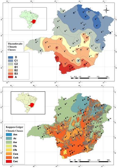
Figure 1.
Climate classifications for Minas Gerais state according to Thornthwaite [35] (source: the authors, 2023) and Köppen classifications [36]. Black pins represent the meteorological station.
2.2. Penman–Monteith FAO Model
The FAO Penman–Monteith equation (FPM) was used to estimate average monthly ET0. This method is described in [34]. It is common practice to use ET0 values estimated by the FPM equation as reference data. The climatological stations used in this study do not provide net solar radiation (Rn) data. The Rn data were obtained from insolation, latitude, day of the year, and other variables. They are calculated using the equations detailed in [26].
Although recommended as a reference method, the equation proposed for FAO has several parameters based on a series of general assumptions about ground cover and vegetation, which means that the FPM equation is a simplification. However, due to the lack of reliable data from lysimeters and the difficulty of handling them, use of the FPM equation is recommended. According to [37], this equation is recommended for estimating ET0 and validating other equations in the absence of experimental measurements; studies that consider FPM targets to train and test models often overlook the implications that arise from this simplification.
2.3. Model Development and Statistical Tests
In this study, different input combinations of the average monthly data were used as inputs to estimate ET0. The input data were geographic coordinates, altitude, month, Tmean, Tmax, Tmin, and RH. In the search for better performance, the four input combinations (In: n is the amount of input data) evaluated in this paper were: (I8) latitude, longitude, altitude, month, Tmean, Tmax, Tmin, and RH; (I6) latitude, longitude, altitude, month, Tmean, and RH; (I3) month, Tmean, and RH; and (I2) Tmean and RH. Combinations were employed to investigate the influence of each meteorological variable on estimation and the resulting impact when a variable was removed. Moreover, average temperature (T) and average relative humidity (RH) data were kept consistent across all combinations, as they are responsible for the energy available in the system and the gradient difference, respectively.
The ANN, RF, SVM, and MLR models were trained for each combination. The models were developed using data from each climate scenario. These combinations were compared with each other in each model.
The predictive quality of each model in terms of variation, precision, accuracy, and performance was evaluated by four statistical criteria. The statistical criteria were mean absolute error (MAE), root-mean-square error (RMSE), coefficient of determination (R2), and Pearson’s correlation coefficient (r) (equations below). MAE and RMSE indicate how close the predicted values were to the observed value. Thus, the accuracy of each model could be predicted. R² represents the percentage of the variation in the dependent variable explained by the independent variable. r indicates the degree of dispersion of the data obtained in terms of the mean.
where Pi is the predicted value (mm), Oi is the observed value (mm), P is the mean of the predicted values (mm), O is the mean of the observed values (mm), and N is the number of data pairs.
2.4. Artificial Neural Networks (ANN)
ANNs have performance characteristics resembling the biology of the human brain. ANNs, in general, have architectures with connections between nodes (neural networks) and methods to determine the connection weights. In this study, an ANN of the feed-forward multilayer perceptron (MLP) type was used [38]. An MLP is a robust choice due to its ability to handle a variety of problems and learn complex nonlinear functions effectively. With multiple hidden layers, MLPs can capture intricate relationships within the data, providing greater flexibility in modeling [12,16]. The training of this ANN involved two phases. In the first phase, or forward pass, the input sign spreads forward layer by layer. In the second phase, or reverse pass, the sign is backpropagated for correction of the error.
ANN was implemented using the Waikato Environment for Knowledge Analysis (WEKA; version 3.8.2 © 1999–2017) developed by the University of Waikato, Hamilton, New Zealand. The input data consisted of different combinations of the latitude, longitude, altitude, month, Tmean, Tmax, Tmin, and RH for each evaluated location, using ET0 as the output variable.
All adjustments were performed by cross-validation. According to [14], the cross-validation approach enables successful results. The method employed in constructing the models was k-fold cross-validation. This technique uses all available data, which is partitioned into k disjoint subsets roughly equal in size. This partitioning is performed by random sampling of the learning set without replacement. The model is then trained k times, using k-1 subsets for training and the remaining subset for validation and to assess its performance. This procedure is repeated until each of the k subsets has served as the validation set. The average of the performance metrics from all of these interactions is considered the cross-validation performance [39]. This methodology was used due to the limited number of climatological stations within the Minas Gerais state. According to [39], K-fold cross-validation is commonly utilized when the quantity of data is limited, as it helps to maximize the utilization of the available data. In this way, this method makes it possible to work with fewer data and obtain optimal results.
The different ANN configurations and number of folds used in cross-validation are shown in Table 2. In this study, models with one or two hidden layers were utilized (Table 2). Initial tests were performed to determine the best-performing model within each input data combination. Various configurations, including different numbers of neurons in the layers, were tested. The architecture with the highest performance for each data input combination was selected (Figure 2).
Table 2.
WEKA configuration in the ANN implementation.
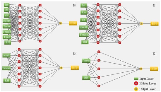
Figure 2.
Network structure scheme built by WEKA to estimate ET0.
However, it is important to note that using multiple hidden layers allows the model to learn more complex representations of the data. While it is possible for a single hidden layer to approximate any function, it may be computationally inefficient or require a large number of neurons in the hidden layer to learn an adequate representation of the data. Additionally, neural networks with a single hidden layer often struggle with generalization, which can lead to inaccurate prediction for unseen data. However, in some situations, it was observed that a single layer performed better than two.
Regarding the initial random assignment of weights, also known as seed, WEKA allows users to change the values as necessary or randomly generate them without the need for an initial introduction. However, if no weight is assigned, the default setting will assign a value of 1 to the seed. Therefore, in this study, the random seed for initialization was set to 1. This allows for consistent comparison of results across different runs of the algorithm and facilitates assessment of the reliability of the results. The other WEKA configuration parameters were kept as standard.
2.5. Support Vector Machine (SVM)
In this study, SVM equations were applied based on Vapnik’s theory [22]. SVMs are separated into two main categories: (i) the classifier model and (ii) the regression model (SVR). SVR is used to take a hyperplane suitable for the data used. The distance to any point in this hyperplane shows the error of that point [14]. SVR can be translated into the following equation:
where x is the input data; φ(x) represents a function that can transfer x into high-dimensional feature spaces; and ω (weight vector) and b are coefficients which are estimated by minimizing the regularized risk function. The error function in the SVM model is minimized based on the mentioned constraints in the equation below. Further details on the application of SVM can be found in [40].
where C is the capacity or penalty parameter, yi is the estimated output by SVM, and ξi and ξ*i are slack variables which must satisfy the function constraints. The SVM model changes the scale of the problem by using kernel functions to solve non-linear problems. SVM provides four different kernel functions: sigmoid, linear, polynomial, and radial basis functions. In this study, during SVM modelling, all kernel functions were tested. The linear kernel function proved to be more efficient for estimating ET0. The linear kernel function is as follows:
where xi and xj are vectors in the input space. The SVM was implemented by WEKA. The input data consisted of different combinations (I8, I6, I4 and I2) and were evaluated in the three different scenarios. The WEKA configuration parameters in the SVM implementation were: SVM Type, ϵ-SVR; cost parameter C, 0.01. The random seed for initialization was set to 1, and gamma was not utilized as the kernel function was linear. The other WEKA configuration parameters were kept as standard for the libsvm library. The libsvm library simplifies the use of SVM in various studies and has enabled its application in pattern recognition and other machine-learning fields [39]. Eighteen folds of the sample set were used in cross-assessment. The same WEKA configuration parameters were used for all input data combinations and in all scenarios.
2.6. Random Forest (RF)
RF is an ensemble learning technique based on a collection of tree predictors [41]. It is a combination of many predictor trees (forest), in which each tree is generated from a random vector and sampled independently, with the same distribution for all trees in the forest. According to [20], there are three simple steps to building an RF model: (i) build n bootstrap samples from the original data; (ii) build an unpruned regression tree; and (iii) predict new data by aggregating the predictions of the n. More details can be found in [20,42] regarding the representation of the steps used in the RF model following the resampling strategy.
RF was implemented by WEKA. The WEKA configuration that resulted in the greatest predictive capacity was a bag size of 100 (the size of each bag, as a percentage of the training set size); 500 iterations (the number of trees in the random forest); unlimited depth for individual trees (as standard); and a random seed for initialization of 1. The other WEKA configuration parameters were kept as standard. All adjustments were performed with cross-validation, and twenty folds of the sample set were used; therefore, the number of splits is not specified. The same WEKA configuration parameters were used in all input data combinations and in all scenarios as they yielded the best results. Adjustments to the hyperparameters aimed at minimizing the root-mean-square error (RMSE) of the validation set. The methodology applied was similar to that employed by [43]; however, it did not involve a separate test set due to the cross-validation approach.
2.7. Multiple Linear Regression (MLR)
MLR was developed to estimate ET0 based on different combinations of the independent variables. The base regression equation can be expressed as:
where Yi is the dependent variable (ET0); lat, lon, alt, month, Tmean, Tmax, Tmin, and RH are independent variables; and β0, β1, β2, β3, β4, β5, β6, β7, and β8 are the regression coefficients.
MLR was implemented using WEKA. The attribute selection method used in the WEKA configuration was the M5 method. This method initially builds the MLR model with all independent variables. Then, the independent variables with the smallest standardized coefficients are removed stepwise until no improvement is observed in the estimate of the error given by the Akaike information criterion (AIC). The AIC seeks the best model in terms of complexity and performance. This technique evaluates different models relative to each other; therefore, when adding more parameters, the AIC of the model may show inadequate performance [44]. The other WEKA configuration parameters were kept as standard. Eighteen folds of the sample set were used in cross-assessment. The same WEKA configuration parameters were used for all input data combinations and in all scenarios.
3. Results and Discussion
The results presented in this study are essential for more adequate water management, since accurate estimation of ET0 is fundamental for water demand quantification. Moreover, the use of different estimation techniques and combinations of input data in the models allowed us to obtain important results at different spatial scales. It must be noted that while daily ET0 values are useful for conducting irrigation, monthly ET0 provides an overview of how much water is required to maintain plant health over a longer period, such as a month or growth cycle. Monthly ET0 is particularly valuable in irrigation planning, as it helps water managers, designers, development planners, and farmers estimate the total water requirements for a successful harvest and make accurate decisions.
According to the results, it was possible to observe linear correlations between the input data and ET0, with the variables Tmean, Tmax, and Tmin showing the best correlation (Figure 3). The other variables have a low (lat, alt and RH) or no (lon and month) correlation with ET0. Behavior inversely proportional to ET0 was observed for the lat, alt, and RH variables. Higher latitudes tend to be cooler regions, with less energy available for the ET0 process. An increase in altitude also results in a decrease in temperature according to the vertical thermal gradient in the troposphere. An increase in RH increases the potential gradient, increasing the water transfer rate from the soil–plant system to the atmosphere. However, proportional behavior was observed between the Tmean, Tmax, and Tmin variables and ET0. An increase in Tmean, Tmax, or Tmin results in more energy being available for ET0. The authors of [14] observed the same behavior in the variables Tmean, Tmax, Tmin, and RH when estimating ET0. The variables Tmean, Tmax, and Tmin were all highly correlated with ET0, and the RH mean was the least correlated variable.
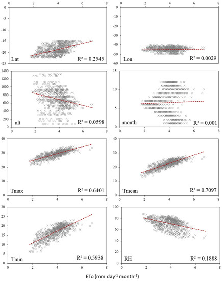
Figure 3.
Correlation analysis between ET0 and each input variable.
In this way, the capability of machine-learning approaches using the variables mentioned above was investigated in different conditions and scenarios. The ANN, RF, SVM, and MLR statistical performance indicators for estimating ET0 in any location within the Minas Gerais state (SI: data from the 56 climatological stations—100% of the input data available) are presented in Table 3.
Table 3.
Statistical performance indicators of the ANN, RF, SVM, and MLR models in SI.
All the models developed with the I8 and I6 input combinations exhibited better performance than versions developed with I3 and I2. The lowest predictive capacity was observed when the RF model was used with the I8 input combination. The greatest predictive capacity, in SI, was observed when the RF and ANN models were used with the I6 and I8 input combinations, respectively. The SVM and MLR models exhibited better performance than ANN and RF when only Tmean and RHmean (I2) were used as input data.
When comparing combination I8 with I6, the average r, MAE, and RMSE values for all models do not show high variation. Removal of the geographic coordinates (I6 to I3) resulted in greater performance reduction for the SVM and MLR models. The greatest impact on performance was observed for ANN and RF when the month variable was removed (I3 to I2). Average r decreased by 8%; MAE and RMSE increased by 52.2% and 43.9%, respectively. The removal of month did not impact the SVM and MLR models’ performance.
In the case of SII, a scenario in which the state of Minas Gerais was divided into two areas (Tho1 and Tho2), the statistical performance indicators of the models used in ET0 estimation are shown in Table 4.
Table 4.
Statistical performance indicators of the ANN, RF, SVM, and MLR models in SII.
Tho1 and Tho2 had 48.2% and 51.8%, respectively, of the data available as input data. The highest predictive capacities in the Tho1 and Tho2 areas were observed when the ANN model was used with the I8 input combination and RF model was used with the I6 input combination, respectively. The removal of Tmax and Tmin input data (I6) did not increase the models’ predictive capacities in the Tho1 area, except for the RF model. This behavior is similar to that observed in SI. However, all models performed better in the Tho2 area when the I6 input combination was used (better results).
Removal of the month variable (I3 to I2) resulted in the greatest impact on the ANN and RF models’ quality. When comparing combination I8 with I3, the average r values of the ANN and RF models decreased by 7.2% and 5.7%, respectively. The MAE values of the ANN and RF models increased by 36.4% and 31.6%, respectively. However, no expressive variation was observed in the performance of the SVM and MLR models.
In the case of SIII, the statistical performance indicators of the models for this scenario are presented in Table 5, where the Minas Gerais state was divided in areas K1 and K2, which were characterized by 62.5% and 37.5% of the climatological stations, respectively.
Table 5.
Statistical performance indicators of the ANN, RF, SVM, and MLR models in SIII.
In general, the ANN and RF models were better than the SVM and RLM models with the input combinations I8, I6, and I3. When the I2 combination was used, the SVM and RLM models were superior. The model with highest predictive capacity in the K1 area was ANN with the I8 input combination. The RF model with the I6 input combination showed the highest predictive capacity in the K2 area.
In the K1 area, removal of the month variable resulted in the greatest impact on the ANN and RF models’ performance. Removal of the alt, lat, and lon variables resulted in the highest impact on the SVM and MLR models’ performance. In the K2 area, the behavior of RF, SVM, and MLR was similar to that observed in the K1 area. However, withdrawal of the alt, lat, and lon variables resulted in the highest impact on ANN in the K2 area.
The ANN and RF models showed greater predictive capacity in all scenarios when compared with the SVM and MLR models. This high capacity is achieved with the data input combinations I8 and I6. Both models had similar performance, but, on average, RF showed slight superiority. In [12,15], the authors evaluated the performance of different machine-learning models in ET0 estimation in Brazil. In these studies, it was observed that, in general, ANN performed slightly better than the other traditional machine-learning models (i.e., RF and extreme gradient boosting—XGBoost). However, in some studies, the RF model performed slightly better than other models (i.e., generalized regression neural networks—GRNN) in estimating ET0 [20,45]. There are papers suggesting better performance than other machine-learning models in different situations and regions [24,46]. Therefore, there is a need for studies that address more than one model.
The SVM and MLR models showed similar statistical indices and responses in all scenarios. These results can be explained by the use of the linear kernel function in SVM, which probably presented behavior similar to an MLR. Tests with the nonlinear kernel function did not result in improvements in prediction. Possibly, the data used does not present complexity that justifies the use of SVM.
The SVM and MLR models showed greater predictive capacity in all scenarios when the input data were limited to only Tmean and RH (I2). This result may indicate a low predictive capacity of the ANN and RF models in situations of low variability in the input data. This low variability may hinder the search for patterns that justify variations in ET0.
In some scenarios, the removal of Tmax and Tmin improved the ET0 estimation results. According to [14], the authors observed an increase in the accuracy of the support vector regression (SVR) and Gaussian process regression (GPR) models with the removal of some input data, including Tmax and Tmin.
Although Tmax and Tmin showed a good correlation with ET0 (Figure 3), the weight of Tmax and Tmin is diluted in the calculation of Tmean used in the calculation of ET0. Thus, adding Tmax and Tmin can make ET0 estimation more complex or confusing. This fact can decrease the accuracy of the models, and the removal of this input data can improve the prediction. Determining the input data is critical to the success of the models. This selection can facilitate the training and testing process, improving the understanding of the system [47,48]. However, this result shows that linear regression alone is not sufficient to decide which input data should be removed in order to increase predictive performance.
When the independent variables lat, lon, and alt were removed (I3), a reduction in the statistical indexes of all models was observed. These variables are related to the spatial location of the observed data. Although the correlation observed between these variables and ET0 is low (Figure 4), the joint removal of these data negatively impacted the model’s performance. The air temperature and solar radiation variables are among the main data impacting ET0 [1,46]. Several studies have indicated the influence of lat, lon, and alt variables on air temperature and solar radiation [49,50]. Therefore, variations in lat, lon, and alt may indirectly impact ET0. This can explain these observed results.
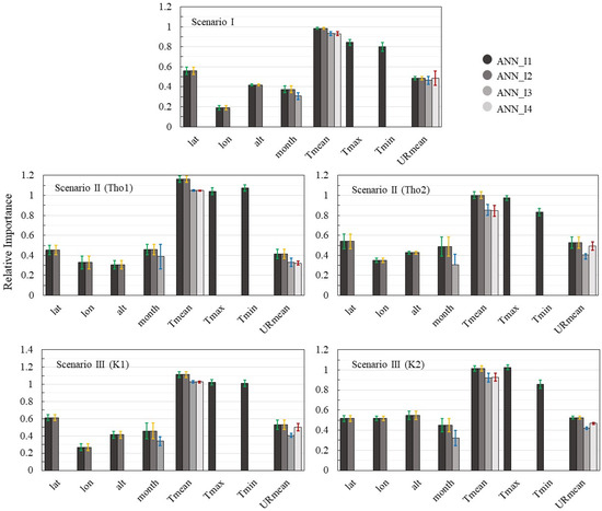
Figure 4.
Importance of the input variables in ANN models. The bars represent standard deviation.
The division of the input data into two areas with climatic similarity aimed to increase the performance of the models. The division presented in SII and SIII managed to slightly increase the capacities of the models in relation to SI. However, this increase was only observed in the Tho1 and K1 areas. Thus, we can infer that, although the division into areas with climatic similarity can reduce the amount of input data for training, in some situations this division is valid, and the models can respond more accurately. Machine-learning models developed for broader scenarios (e.g., SI) typically have reduced predictive capacity due to the high nonlinearity and low similarity of their input data; however, these models have greater ability to generalize [24]. According to [12], although the models developed locally perform better, these models may have low predictive capacity when used in other regions, since they may be highly specific to the location.
Regarding the importance of each input variable to the response variable of the evaluated algorithms, WEKA was used to select the attributes (Figure 4, Figure 5 and Figure 6). Attributes were selected using the “ClassifierAttributeEval” tool associated with the “Ranker” method. These tools rank attributes by their individual evaluations. Correlation coefficient was the measure used to evaluate the performance of attribute combinations in the Ranker configuration. The same ranking method in WEKA was used by [51] in order to verify the importance of each input variable in solar radiation prediction.
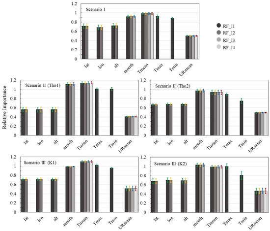
Figure 5.
Importance of the input variables in RF models. The bars represent standard deviation.
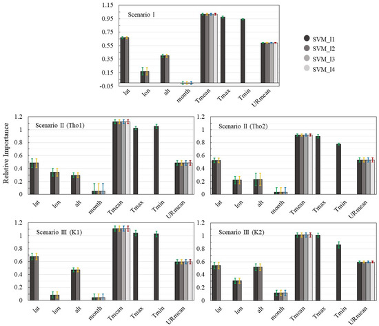
Figure 6.
Importance of the input variables in SVM models. The bars represent standard deviation.
Different ANN settings were used for different input data (Table 2). These ANN settings resulted in different weights for each input attribute (Figure 4). However, similar behavior was observed in the different configurations. In all scenarios, Tmean, Tmax, and Tmin had greater weight in producing the estimate. In SIII K2, the relative importance of Tmax surpassed Tmed (Figure 4). This result may explain the decrease in ANN’s performance in this scenario when Tmax and Tmin were removed (Table 4). The variables lat and month had a similar weight in all scenarios. Although similar, the removal of the month variable resulted in a greater reduction in ANN’s performance when compared with the removal of the variables lat, lon, and alt.
The ranked values of each input variable in RF are shown in Figure 5. The Tmean and month variables had a higher weight in the ET0 estimate. In SII Tho1 and SIII K2, the month variable was more important than the Tmean variable. This result may explain the drop in the RF model’s performance when it removed the month variable (I3 to I2). The Tmax and Tmin variables also had a high weight in the ET0 estimate. However, the removal of these variables increased the capacity of the RF model as observed (Table 3, Table 4 and Table 5) and discussed previously.
The relative importance of each input variable in SVM is shown in Figure 6. It was possible to observe that the Tmean, Tmax, and Tmin variables had a higher weight in the ET0 estimate, followed by HR and lat. The month variable was of low importance in the ET0 estimate. In SI, the month showed a negative weight. Therefore, this input data can negatively impact the ET0 estimate. In the performance results for the SVM model (Table 3, Table 4 and Table 5), there was no significant variation in performance when the month variable was removed. Both results make it possible to highlight that, for this region, the month variable does not contribute to the performance of the SVM model.
Although each model has a different pattern in the ranking of the input variables (Figure 4, Figure 5 and Figure 6), air temperature was the most important attribute. The observed correlation between air temperature and ET0 (Figure 4) may explain the importance of air temperature in this estimate. This behavior was not observed in SIII K2 or SII Tho2. However, in these scenarios, no significant difference was observed between the month and Tmean variables. Studying the ranking of the importance of meteorological variables based on the RF method, the three most important variables were insolation (n), Tmax, and RH [20]. The high relative importance observed corroborates the results of the present study.
The other variables presented different weights according to each model applied. These results indicate a peculiarity of the models. Hence, new research and applications can be based on these results, choosing the best method to suit the conditions of the input data. However, it is recommended that the models be previously experimented with using different input data; as noted, some variables may have a relatively high weight in the ET0 estimate, but their use can decrease the predictive performance of the model. This behavior was observed when using the RF model. In this model, removal of the variables Tmax and Tmin increased predictive capacity, although these variables have shown high relative importance.
It is important to note that the month variable was highly important in estimation with RF. However, low importance was observed when the SVM model was used, since this variable was not correlated with ET0 (Figure 3). These results highlight the need for more techniques to select the meteorological variables used in modeling. Linear regression alone is not sufficient to identify the relevance of the input data. Furthermore, different models may present different behaviors regarding classification of the importance of the input variable and still present satisfactory results.
Differently from the evaluation of the importance of the ANN, RF, and SVM attributes, for the MLR method, the attribute selection method was applied (the M5 method), which indicates the importance of each input attribute in the generated model. The adjusted coefficients are shown in Table 6. It was observed that, in some models, the method used (the M5 method) excluded the month variable. This behavior indicates a low importance of this variable in the MLR estimate. This result was similar to that observed in the analysis of the importance of the input variables in SVM. The exclusion of lat and Tmax was also observed in some cases.
Table 6.
Coefficients of the multiple linear regression models in SI, SII, and SIII.
The results presented in this study reveal that, for locations in Minas Gerais state, these models can be used safely. The ANN and RF models are recommended to estimate ET0 when considering a wider range of input data, as they have better predictive capacity in this situation. The SVM and MLR models are recommended in situations where only temperature and relative humidity data are available. However, between these two models, MLR is recommended because it requires less computational effort. These models, although they have a high predictive capacity, cannot be perfect. Other meteorological variables not considered as input data (e.g., solar radiation, wind speed, and vapour-pressure deficit) and other factors (e.g., data recorded in error) contributed to a decrease in the predictive capacity of these models.
No statistical method or machine-learning method can produce results that are the same as the observed and/or recorded data. There will always be some error, no matter how small. Therefore, it is important that the meteorological stations function continuously. As in all studies, some limitations were noted in this study. One of the main limitations is related to difficulties in the availability of quality meteorological data. The malfunction and limited collection of meteorological data has been a limitation in several countries. Another limitation that can be observed is the difficulty and complexity of using some models. In this context, it is recommended to evaluate and use models with good results and that present greater simplicity in their use.
The models developed in this study are expected to help decision-making by different professionals, mainly farmers. Agricultural companies are responsible for a considerable part of the Brazilian gross domestic product [52], and the Minas Gerais state had the third-largest gross domestic product in Brazil in 2018 [33]. The results of these models can assist in irrigation management, climatic zoning, and the construction of productivity models, among other applications. In addition, the approaches used in the present study have the potential to benefit the development of other types of models and studies from other regions.
4. Conclusions
The results and information presented in this study are important for planning and determining the use of the best model to estimate ET0 for a region with limited climate data. The use of input data combination I6 (alt, lat, lon, month, Tmean, and RH) in the scenarios SI, SII, and SIII provided in general the best results in ET0 estimation between the evaluated models, so this data combination is recommended to be used. The RF and ANN models presented the highest predictive ability for the ET0 estimate. Both models, in best-case scenarios, with the input data combination I6 or I8, explain more than 96% of the variability of the variables estimated using the independent dataset. If experimental data are available, machine-learning algorithms represent a powerful tool able to provide accurate predictions. The SVM and MLR models are recommended for all scenarios in situations with limited climatic data where only air temperature and relative humidity data are available. Although dividing into scenarios results in less input data for model training, the SII and SIII scenarios showed slightly better results in the southern areas of the Minas Gerais state.
Air temperature was the meteorological input variable that presented the greatest relative importance, while the month variable presented the greatest variation in importance in relation to the model used. Therefore, it is concluded that although temperature is fundamental for the estimation of ET0, other variables can present different levels of importance in the prediction of ET0.
The results presented in this study contribute relevant information, and, together with other studies, can serve as a basis for the estimation of reference evapotranspiration. However, new studies are necessary in order to evaluate new models and their performance with limited climate data, based on other machine-learning algorithms that contemplate different climatic conditions and that subsequently take into account the effects of climate change.
Author Contributions
Conceptualization, P.A.B.d.S. and F.S.; methodology and formal analysis, L.G.d.C., V.B.d.S.B., D.B.M., and G.A.e.S.F.; data curation, P.A.B.d.S., D.B.M., and F.S.; writing—original draft preparation, P.A.B.d.S.; writing—review and editing, L.C., G.B., G.R., and F.S.; visualization, D.B.M. and V.B.d.S.B.; supervision, G.A.e.S.F., L.C., G.B., G.R., and F.S.; project administration, P.A.B.d.S. All authors have read and agreed to the published version of the manuscript.
Funding
The authors would like to thank the Coordination for the Improvement of Higher Education Personnel (CAPES—Finance Code 001) for the research and study grants.
Data Availability Statement
The data presented in this study are available on request from the corresponding author. The data are not publicly available.
Conflicts of Interest
The authors declare no conflict of interest.
References
- Souza, L.S.B.; Silva, M.T.L.; Alba, E.; Moura, M.S.B.; Cruz Neto, J.F.; Souza, C.A.A.; Silva, T.G.F. New method for estimating reference evapotranspiration and comparison with alternative methods in a fruit-producing hub in the semi-arid region of Brazil. Theor. Appl. Climatol. 2022, 149, 593–602. [Google Scholar] [CrossRef]
- Wen, X.; Si, J.; He, Z.; Wu, J.; Shao, H.; Yu, H. Support-vector-machine-based models for modeling daily reference evapotranspiration with limited climatic data in extreme arid regions. Water Resour. Manag. 2015, 29, 3195–3209. [Google Scholar] [CrossRef]
- Yassin, M.A.; Alazba, A.A.; Mattar, M.A. Artificial neural networks versus gene expression programming for estimating reference evapotranspiration in arid climate. Agric. Water Manag. 2016, 163, 110–124. [Google Scholar] [CrossRef]
- Kumar, M.; Raghuwanshi, N.S.; Singh, R.; Wallender, W.W.; Pruitt, W.O. Estimating evapotranspiration using artificial neural network. J. Irrig. Drain. Eng. 2002, 128, 224–233. [Google Scholar] [CrossRef]
- Ning, M.; Jozsef, S.; Zhang, Y. Calibration-free complementary relationship estimates terrestrial evapotranspiration globally. Water Resour. Res. 2021, 57, e2021WR029691. [Google Scholar]
- Yu, L.; Qiu, G.Y.; Yan, C.; Zhao, W.; Zou, Z.; Ding, J.; Xiong, Y. A global terrestrial evapotranspiration product based on the three-temperature model with fewer input parameters and no calibration requirement. Earth Syst. Sci. Data 2022, 14, 3673–3693. [Google Scholar] [CrossRef]
- Almorox, J.; Quej, V.H.; Martí, P. Global performance ranking of temperature-based approaches for evapotranspiration estimation considering Köppen climate classes. J. Hydrol. 2015, 528, 514–522. [Google Scholar] [CrossRef]
- Yang, Q.; Ma, Z.; Zheng, Z.; Duan, Y. Sensitivity of potential evapotranspiration estimation to the Thornthwaite and Penman–Monteith methods in the study of global drylands. Adv. Atmos. Sci. 2017, 34, 1381–1394. [Google Scholar] [CrossRef]
- Ewaid, S.H.; Abed, S.A.; Al-Ansari, N. Crop water requirements and irrigation schedules for some major crops in Southern Iraq. Water 2019, 11, 756. [Google Scholar] [CrossRef]
- Xiang, K.; Li, Y.; Horton, R.; Feng, H. Similarity and difference of potential evapotranspiration and reference crop evapotranspiration—A review. Agric. Water Manag. 2020, 232, 106043. [Google Scholar] [CrossRef]
- Benali, L.; Notton, G.; Fouilloy, A.; Voyant, C.; Dizene, R. Solar radiation forecasting using artificial neural network and random forest methods: Application to normal beam, horizontal diffuse and global components. Renew. Energy 2019, 132, 871–884. [Google Scholar] [CrossRef]
- Ferreira, L.B.; Cunha, F.F.; Oliveira, R.A.; Fernandes Filho, E.I. Estimation of reference evapotranspiration in Brazil with limited meteorological data using ANN and SVM–A new approach. J. Hydrol. 2019, 572, 556–570. [Google Scholar] [CrossRef]
- Malik, A.; Kumar, A.; Ghorbani, M.A.; Kashani, M.H.; Kisi, O.; Kim, S. The viability of co-active fuzzy inference system model for monthly reference evapotranspiration estimation: Case study of Uttarakhand State. Hydrol. Res. 2019, 50, 1623–1644. [Google Scholar] [CrossRef]
- Sattari, M.T.; Apaydin, H.; Band, S.S.; Mosavi, A.; Prasad, R. Comparative analysis of kernel-based versus ANN and deep learning methods in monthly reference evapotranspiration estimation. Hydrol. Earth Syst. Sci. 2021, 25, 603–618. [Google Scholar] [CrossRef]
- Ferreira, L.B.; Da Cunha, F.F. New approach to estimate daily reference evapotranspiration based on hourly temperature and relative humidity using machine learning and deep learning. Agric. Water Manag. 2020, 234, 106–113. [Google Scholar] [CrossRef]
- Yin, Z.; Wen, X.; Feng, Q.; He, Z.; Zou, S.; Yang, L. Integrating genetic algorithm and support vector machine for modeling daily reference evapotranspiration in a semi-arid mountain area. Hydrol. Res. 2017, 48, 1177–1191. [Google Scholar] [CrossRef]
- Martí, P.; González-Altozano, P.; Gasque, M. Reference evapotranspiration estimation without local climatic data. Irrig. Sci. 2011, 29, 479–495. [Google Scholar] [CrossRef]
- Nourani, V.; Elkiran, G.; Abdullahi, J. Multi-station artificial intelligence based ensemble modeling of reference evapotranspiration using pan evaporation measurements. J. Hydrol. 2019, 577, 123958. [Google Scholar] [CrossRef]
- Feng, Y.; Cui, N.; Gong, D.; Zhang, Q.; Zhao, L. Evaluation of random forests and generalized regression neural networks for daily reference evapotranspiration modelling. Agric. Water Manag. 2017, 193, 163–173. [Google Scholar] [CrossRef]
- Wang, S.; Lian, J.; Peng, Y.; Hu, B.; Chen, H. Generalized reference evapotranspiration models with limited climatic data based on random forest and gene expression programming in Guangxi, China. Agric. Water Manag. 2019, 221, 220–230. [Google Scholar] [CrossRef]
- Zhou, X.; Zhu, X.; Dong, Z.; Guo, W. Estimation of biomass in wheat using random forest regression algorithm and remote sensing data. Crop. J. 2016, 4, 212–219. [Google Scholar]
- Vapnik, V. The Nature of Statistical Learning Theory; Springer: Berlin/Heidelberg, Germany, 2013; p. 188. [Google Scholar]
- Mohammadrezapour, O.; Piri, J.; Kisi, O. Comparison of SVM, ANFIS and GEP in modeling monthly potential evapotranspiration in an arid region (Case study: Sistan and Baluchestan Province, Iran). Water Supply 2019, 19, 392–403. [Google Scholar] [CrossRef]
- Shiri, J.; Nazemi, A.H.; Sadraddini, A.A.; Landeras, G.; Kisi, O.; Fard, A.F.; Marti, P. Comparison of heuristic and empirical approaches for estimating reference evapotranspiration from limited inputs in Iran. Comput. Electron. Agric. 2014, 108, 230–241. [Google Scholar] [CrossRef]
- Valipour, M.; Gholami Sefidkouhi, M.A.; Raeini−Sarjaz, M. Selecting the best model to estimate potential evapotranspiration with respect to climate change and magnitudes of extreme events. Agric. Water Manag. 2017, 180, 50–60. [Google Scholar] [CrossRef]
- Wang, Z.; Xie, P.; Lai, C.; Chen, X.; Wu, X.; Zeng, Z.; Li, J. Spatiotemporal variability of reference evapotranspiration and contributing climatic factors in China during 1961–2013. J. Hydrol. 2017, 544, 97–108. [Google Scholar] [CrossRef]
- Dou, X.; Yang, Y. Evapotranspiration estimation using four different ma-chine learning approaches in different terrestrial ecosystems. Comput. Electron. Agric. 2018, 148, 95–106. [Google Scholar] [CrossRef]
- Pozníková, G.; Fischer, M.; van Kesteren, B.; Orság, M.; Hlavinka, P.; Žalud, Z.; Trnka, M. Quantifying turbulent energy fluxes and evapotranspiration in agricultural field conditions: A comparison of micrometeorological methods. Agric. Water Manag. 2018, 209, 249–263. [Google Scholar] [CrossRef]
- Tang, D.; Feng, Y.; Gong, D.; Hao, W.; Cui, N. Evaluation of artificial intelligence models for actual crop evapotranspiration modeling in mulched and non-mulched maize croplands. Comput. Electron. Agric. 2018, 152, 375–384. [Google Scholar] [CrossRef]
- Zhang, Z.; Gong, Y.; Wang, Z. Accessible remote sensing data based reference evapotranspiration estimation modelling. Agric. Water Manag. 2018, 210, 59–69. [Google Scholar] [CrossRef]
- Granata, F. Evapotranspiration evaluation models based on machine learning algorithms—A comparative study. Agric. Water Manag. 2019, 217, 303–315. [Google Scholar] [CrossRef]
- Chen, Z.; Zhu, Z.; Jiang, H.; Sun, S. Estimating daily reference evapotran-spiration based on limited meteorological data using deep learning and classical machine learning methods. J. Hydrol. 2020, 591, 125286. [Google Scholar] [CrossRef]
- IBGE. Instituto Brasileiro de Geografia e Estatística. 2022. Available online: https://cidades.ibge.gov.br/brasil/mg (accessed on 28 April 2022).
- Allen, R.G.; Pereira, L.S.; Raes, D.; Smith, M. Crop Evapotranspiration—Guidelines for Computing Crop Water Requirements; FAO Irrigation and Drainage Paper 56; FAO: Rome, Italy, 1998; 297p. [Google Scholar]
- Thornthwaite, C.W. An approach toward a rational classification of climate. Geogr. Rev. 1948, 38, 55–94. [Google Scholar] [CrossRef]
- Alvares, C.A.; Stape, J.L.; Sentelhas, P.C.; Gonçalves, J.D.M.; Sparovek, G. Köppen’s climate classification map for Brazil. Meteorol. Z. 2013, 22, 711–728. [Google Scholar] [CrossRef] [PubMed]
- Martí, P.; González-Altozano, P.; López-Urrea, R.; Mancha, L.A.; Shiri, J. Modeling reference evapotranspiration with calculated targets. Assessment and implications. Agric. Water Manag. 2015, 149, 81–90. [Google Scholar] [CrossRef]
- Fausett, L. Fundamentals of Neural Networks: Architectures, Algorithms, and Applications; Pearson Education India Editora: Chennai, India, 1994; 461p. [Google Scholar]
- Berar, D. Cross-validation. In Encyclopedia of Bioinformatics and Computational Biology; Elsevier: Amsterdam, The Netherlands, 2019; pp. 542–545. [Google Scholar]
- Chang, C.C.; Lin, C.J. LIBSVM: A library for support vector machines. ACM Trans. Intell. Syst. Technol. 2011, 2, 1–27. [Google Scholar] [CrossRef]
- Xu, Y.; Knudby, A.; Ho, H.C. Estimating daily maximum air temperature from MODIS in British Columbia, Canada. Int. J. Remote Sens. 2014, 35, 8108–8121. [Google Scholar] [CrossRef]
- Wang, H.; Lei, M.; Chen, Y.; Li, M.; Zou, L. Intelligent identification of maceral components of coal based on image segmentation and classification. Appl. Sci. 2019, 9, 3245. [Google Scholar] [CrossRef]
- Schumacher, B.L.; Burchfield, E.K.; Bean, B.; Yost, M.A. Leveraging Important Covariate Groups for Corn Yield Prediction. Agriculture 2023, 13, 61. [Google Scholar] [CrossRef]
- Samadianfard, S.; Asadi, E.; Jarhan, S.; Kazemi, H.; Kheshtgar, S.; Kisi, O.; Manaf, A.A. Wavelet neural networks and gene expression programming models to predict short-term soil temperature at different depths. Soil Tillage Res. 2018, 175, 37–50. [Google Scholar] [CrossRef]
- Feng, Q.; Wen, X.; Li, J. Wavelet analysis-support vector machine coupled models for monthly rainfall forecasting in arid regions. Sustain. Water Resour. Manag. 2015, 29, 1049–1065. [Google Scholar] [CrossRef]
- Mehdizadeh, S.; Behmanesh, J.; Khalili, K. Using MARS, SVM, GEP and empirical equations for estimation of monthly mean reference evapotranspiration. Comput. Electron. Agric. 2017, 139, 103–114. [Google Scholar] [CrossRef]
- Bowden, G.J.; Dandy, G.C.; Maier, H.R. Input determination for neural network models in water resources applications. Part 1—Background and methodology. J. Hydrol. 2005, 301, 75–92. [Google Scholar]
- Maier, H.R.; Dandy, G.C. Neural networks for the prediction and forecasting of water resources variables: A review of modelling issues and applications. Environ. Model Softw. 2000, 15, 101–124. [Google Scholar] [CrossRef]
- Alvares, C.A.; Stape, J.L.; Sentelhas, P.C.; Moraes Gonçalves, J.L. Modeling monthly mean air temperature for Brazil. Theor. Appl. Climatol. 2013, 113, 407–427. [Google Scholar] [CrossRef]
- Ozgoren, M.; Bilgili, M.; Sahin, B. Estimation of global solar radiation using ANN over Turkey. Expert. Syst. Appl. 2012, 39, 5043–5051. [Google Scholar] [CrossRef]
- Yadav, A.K.; Malik, H.; Chandel, S.S. Selection of most relevant input parameters using WEKA for artificial neural network based solar radiation prediction models. Renew. Sust. Energ. Rev. 2014, 31, 509–519. [Google Scholar] [CrossRef]
- Brugnaro, R.; Bacha, C.J.C. Analysis of increased participation of agriculture in the Brazilian GDP from 1994 a 2004. In Proceedings of the Congress of the European Regional Science Association, Volos, Greece, 30 August–3 September 2006; Volume 46, p. 19. [Google Scholar]
Disclaimer/Publisher’s Note: The statements, opinions and data contained in all publications are solely those of the individual author(s) and contributor(s) and not of MDPI and/or the editor(s). MDPI and/or the editor(s) disclaim responsibility for any injury to people or property resulting from any ideas, methods, instructions or products referred to in the content. |
© 2023 by the authors. Licensee MDPI, Basel, Switzerland. This article is an open access article distributed under the terms and conditions of the Creative Commons Attribution (CC BY) license (https://creativecommons.org/licenses/by/4.0/).