Abstract
Different varieties of fresh lotus seeds have varying levels of amylose content. It has a direct impact on the following processing and final product quality, so the non-destructive detection of amylose content is meaningful before lotus seed production. This study proposed a non-destructive method to detect the amylose content of fresh lotus seeds. Hyperspectral images of 120 fresh lotus seeds of three different varieties were obtained, and different pretreatments were applied to the average spectra obtained from the region of interest (ROI). The calibration and prediction set were divided by the sample set joint x–y distances algorithm (SPXY). Then, the partial lease square regression (PLSR) method was established for modeling, with Savitzky–Golay pretreatment-based PLSR showing the best results. To further improve the stability of the predictive model, different methods of feature variables selection were compared. The results showed that the best PLSR model was established with the inputs of 15 feature bands selected from 472 bands by the successive projection algorithm (SPA). The correlation coefficient of the prediction set (Rp), root mean square error of the prediction set (RMSEP), and residual predictive deviation (RPD) were 0.890, 15.154 mg g−1, and 2.193, respectively. Meanwhile, this study visualized the amylose content distribution maps from which it could estimate the content level directly. This study could provide a reference for further development of portable detection equipment for the amylose content of fresh lotus seeds.
1. Introduction
Lotus, a perennial herbaceous aquatic plant of the genus Nelumbo, is found in Asia (Nelumbo nucifera Gaertn.) and America (Nelumbo lutea) [1]. Lotus seed is the mature seed from the seed lotus. As the shelf-life of fresh lotus seeds is short, only some of the lotus seeds are consumed fresh; the majority are processed into various products, such as dried lotus, lotus juice, canned lotus, and lotus porridge, among others [2].
Lotus seeds have abundant starch; amylose is a type of starch made up of linear or helical chains joined by a sequence of α-d-(1,4)-glucosidic linkages [3]. Amylose content can easily affect the quality of lotus production, which can influence water absorption, swelling, solid substance solubility, color, luster, viscosity, and softness of lotus seed production [2,4]. Using lotus seed juice as an example, amylose is easier to retrograde than amylopectin [5]. Therefore, lotus seeds with low amylose content are a better choice for lotus seed juice production. Alternatively, to ensure the quality of the juice product, employ a procedure on the lotus seeds with high amylose content. Studies [6] have shown that the amylose content of lotus seeds varied greatly, not only among different lotus cultivars. So, it is necessary to detect its content before processing to improve production quality.
The traditional method to detect amylose content is the iodine colorimetric method [7], which is both time-consuming and labor-wrecking, as the sample pretreatment often takes more than 16 h. Obviously, the traditional amylose detection methods are difficult in batch detection, and are not suitable for industrial production and processing. To tackle this issue, some researchers have explored the use of the spectral non-destructive method for amylose content detection in powder form. For example, Fertig et al. [8] determined the amylose content in starch mixture by near-infrared (NIR) spectroscopy at 1700–1800 nm, while Zhang et al. [9] employed NIR in 1100–2500 nm to analyze the amylose content in rice flour. Peiris et al. [10] developed partial least squares regression (PLSR) models on NIR spectra to estimate starch and amylose contents in intact grain sorghum samples. The calibration model achieved an R2 of 0.84 and an RMSECV of 2.96%, predicting the amylose content with a value of R2 of 0.76 and RMSEP of 2.60%.
Due to advancements in technology, hyperspectral imaging (HIS) has gained popularity for the non-destructive detection of food and agricultural products with rich spectral and image information [11]. HSI technology is effective in internal quality detection and offers spatial substance content analysis. It is an effective means to avoid single-point measurement of spectroscopy. HIS has been widely used in the detection of internal substances, such as soluble solid content [12], fatty acid content [13], phenol [14], and so on. Huang et al. [15] have successfully utilized HSI for the rapid and non-destructive prediction of amylose and amylopectin contents in different sorghum varieties. However, there is still a lack of research on the detection of lotus seed amylose based on HSI technology. And there is potential for HSI or spectroscopy in determining amylose contents in lotus seeds, according to former studies.
HIS has the advantage of being informative, but still contains irrelevant information. It usually needs to adopt different preprocessing methods and feature selection algorithms before modeling in order to reduce the complexity of the model and improve its accuracy [16]. In addition, human interaction with hyperspectral images is essential for image interpretation and analysis [17], so the internal ingredient visualization by rendering them as RGB color images could help to discriminate the amylose content directly or further development of online detection equipment.
This study aims to evaluate the feasibility of hyperspectral imaging to determine the amylose in lotus seeds. By reducing variables and visualizing the amylose content, the detection speed and comprehensibility of the process can be improved, aiding in the processing of lotus seeds.
2. Materials and Methods
2.1. Samples
Lotus seeds at their maturity stage, belonging to three different varieties (Guangchang, Jianxuan, and Xiang), were collected from the institute of lotus seed in Jian Ning, Fujian province, China (116°83′ E, 26°83′ N), along with their cupules. They were transported to the lab immediately through a cold chain and, upon arrival, were stored at 25 °C and 65% relative humidity for 2 h. Subsequently, the Testa Nelumbini of lotus seeds was peeled off. Then, the hyperspectral images were obtained by selecting a total of 120 lotus seeds, with 40 samples for each variety.
2.2. Hyperspectral Imaging System
The hyperspectral imaging system (Figure 1) was manufactured by Shanghai ISUZU Optics Technology Co., Ltd. in Shanghai, China. The spectrograph (ImSpector V10E, SPECIM, Spectral Imaging Ltd. Oulu, Finland) covers the spectral range of 380–1030 nm, and the spectral resolution is 2.8 nm (using a 30 µm slit). The resolution of the CCD camera is 1392 × 1040 (spatial × spectral) pixels. The linear light source contains two 150 W quartz tungsten halogen lamps (Oriel Instruments, Newport Corporation, Irvine, CA, USA). The acquired images were corrected with white and dark references using Equation (1) [18]:
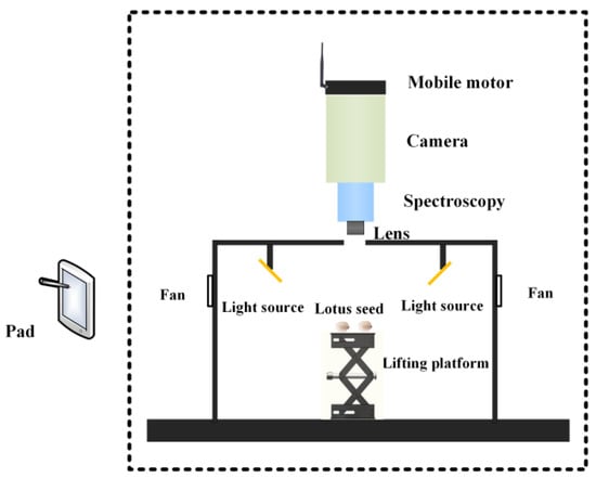
Figure 1.
The hyperspectral imaging system.
Iraw was the collected hyperspectral image, Idark was the dark reference image, and Iwhite was the white reference image (Teflon whiteboard with 99% reflectance).
2.3. Amylose Detection
After obtaining the hyperspectral images, the amylose content of the samples was determined by an amylose kit (Suzhou Comin Biotechnology Co., Ltd., Suzhou, Fujian, China). For each lotus seed, 0.01 g of dried sample was ground in a mortar. After homogenization, extraction, and centrifugation, 20 μL supernatant was placed in a 96-well plate, and a chromogenic agent was added. The absorbance value at 620 nm was measured by a microplate reader (MD SpectraMax M5, Molecular Devices, San Jose, CA, USA), and then the content of lotus seed amylose was calculated as Equation (2). Each sample was determined by three repetitions.
: the absorbance of the sample; : the absorbance of the plate; : the sample volume, 0.02 mL; V2: the extracting solution, 1 mL; W: the sample weight, g.
2.4. Sample Partition
A total of 120 samples were divided into calibration and prediction sets by a sample set partitioning based on joint x–y distances (SPXY) [19]. This partitioning method was developed from the Kennard–Stone algorithm, which is based on the Euclidean distance. SPXY will consider spectral variables and chemical values at the same time. In this study, the ratio of calibration and prediction was set as 2:1. The calculation is as follows:
N is the number of variables in x, and N is the number of samples. and are the kth variables for samples m and n, respectively; N is the number of variables in y and and are the kth variables for samples m and n, respectively; is the Euclidean distance between sample m and n based on spectral variables; is the Euclidean distance between sample m and n based on chemical values; is the distance between sample m and n.
2.5. Spectral Preprocessing
Preprocessing of spectral data is considered an important step before chemometric modeling [20]. Savitzky–Golay smoothing (SG smoothing), standard normal variate (SNV), first-order derivative (1st-D), and multiple scatter correction (MSC) methods were used for the spectra pretreatment. They have been used widely and proved useful in eliminating random noise, removing the multiplicative signal effects, eliminating the baseline drift, and correcting the scattering, respectively [21].
2.6. Variables Selection
Uninformative variable elimination (UVE) is based on the stability of the variable in modeling to eliminate the variables without information [22]. During the UVE calculation, artificial random variables are added to the spectral matrix, and PLSR models are established. Then, the stability of each variable is calculated by the regression coefficient vector of PLSRs. In this study, the cutoff was set as Equation (6) [23]:
is the mean value of the spectra–noise matrix and is the standard deviation of the spectra–noise matrix. t means the single-sided Student t parameter for a probability level and n − 1 freedom degrees. n refers to the total number of random variables. The value of p is usually 0.95, 0.9, 0.85, 0.75, etc. The greater the value of p, the more variables within the cutoff.
The competitive adaptive reweight sampling method (CARS) utilizes the ‘survival of the fittest’ principle to select feature variables [24]. Two main steps constitute CARS wavelength selection. Firstly, employ decreasing function (EDF) is utilized to remove the wavelengths with relatively small absolute regression coefficients by force. Second, adaptive reweighted sampling (ARS) is employed to further eliminate wavelengths competitively. Cross-validation is used to evaluate the variable subset, and the optimal subset has the lowest RMSECV.
A successive projection algorithm (SPA) has been widely used in feature variable selection in spectral detection-related work [21]. Its function is to find a small, representative set of spectral variables to minimize collinearity and eliminate redundant information in the original spectra.
2.7. Partial Least Squares Regression (PLSR)
PLSR is a frequently used algorithm for linearly fitting in chemometrics. The main difference between the PLSR and common multiple linear regression is that it exacts several new variables (also known as components). This method integrates the function of multiple linear regression analysis, correlation analysis, and principal component analysis.
2.8. Data Analysis
Spectral preprocessing is conducted in Unscrambler X 10. 1® (Camo, Oslo, Norway). ENVI (Version 4.7, ITT Visual Information Solutions, Boulder, CO, USA) was applied to collect the images’ spectra from the region of interest (ROI). The variables selection and modeling are carried out in Matlab R2020b (The MathWorks, Natick, MA, USA).
2.9. Evaluation of Model Performance
The evaluation of regression model performance primarily includes the correlation coefficient (R), root mean square error (RMSE), and residual predictive deviation (RPD). RPD was calculated as the ratio of standard deviation (SD) of the reference values to the root mean square error of prediction (RPD = SD/RMSEP). The RPD should be larger than 2.0, and the model will be considered to have a high degree of robustness and may be used for regression prediction [25,26].
3. Results
3.1. Spectra
The ROI of the images yielded average spectra. After removing the wavelengths which have noticeable noises at the beginning and end of the spectra, the spectral curves range from 400 to 1000 nm (472 bands), as shown in Figure 2a. Notably, according to Figure 2b, there is a conspicuous increase in reflectance between 460 and 570 nm, the distinct absorbance in the wavelengths at 450, 680, and 950 nm, respectively. The O-H second overtone is at 950 nm. These ROI spectra were subsequently utilized for additional processing.
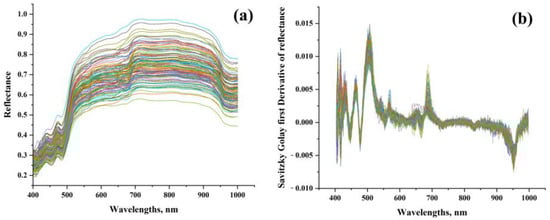
Figure 2.
Average spectra of the 120 samples at ROI. (a) Original spectra; (b) processed spectra by the Savitzky–Golay first derivative.
3.2. Lotus Seeds
Table 1 displays the physical parameters and amylose content of 120 lotus seeds that were split into a calibration set and a prediction set through SPXY partitions, with 80 and 40 samples, respectively. Despite all the samples having similar sizes and weights, there were considerable differences in their amylose content. The minimum amylose content was 46.238 mg g−1, but the maximum was 216.748 mg g−1. The maximum was more than four times bigger than the minimum. These findings indicate the importance of preparing lotus seeds before processing them for other products. The average amylose content did not differ significantly between the calibration and prediction sets after SPXY partitions. Furthermore, the amylose content of the prediction set fell within the range of amylose content. It indicates that after using the SPXY algorithm, the division of the correction set and the prediction set is reasonable.

Table 1.
Statistical results of lotus seed index.
3.3. Spectral Preprocessing
Table 2 presents the results of PLSRs based on the spectra subjected to various pretreatments. Among them, Rc and Rp are the correlation coefficients of the correction set and the prediction set, respectively. The closer their values are to 1, the higher the accuracy of the model. The smaller the root mean square error of calibration (RMSEC) and RMSEP, the more stable the model is. Upon examination of Table 1, it is evident that there is minimal difference in the modeling effect between the PLSR model built with raw data and after four pretreatments. The results of Savitzky–Golay smoothing-based PLSR are very close to deviation-based PLSR, with the former having a slightly lower RMSEP than the latter. We considered that the best PLSR model was established with the spectra after Savitzky–Golay smoothing preprocessing, whose Rc and RMSEC were 0.920 and 14.456 mg g−1, respectively, and Rp and RMSEP were 0.869 and 18.320 mg g−1, respectively. The SG smoothing preprocessed spectra would be used in further analysis.
Table 2.
PLSR model of lotus seed after different pretreatment.
3.4. Feature Variables Selection
Due to the presence of some noise and redundancy in spectral data, the selection of feature variables can not only improve the speed and efficiency of modeling, but also improve the accuracy and stability of the model. The spectra after SG smoothing were adopted in different variable selection methods, whose idea is mainly based on polynomial fitting to eliminate high-frequency noise and low-frequency interference, thereby preserving the main features. UVE is an effective method to eliminate the variables with non-informative variables. Figure 3a calculated the stability of both 472 spectra variables and 472 random variables. When the cutoff was set during the UVE feature selection, only the corresponding variables outside the dashed line were retained. At a probability level of 0.9, the minimum RMSEC was achieved, and 126 variables were selected. Figure 3b displays the operational effect of the UVE algorithm and the distribution of all wavelengths.
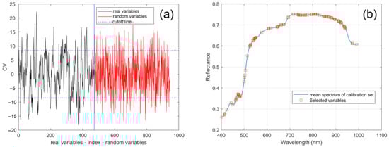
Figure 3.
Feature wavelengths selection by UVE, (a) UVE band selection process, (b) distribution of the wavelengths selected by UVE.
Then, SPA extracted the feature bands based on the SG smoothed spectra and UVE selected variables, respectively. As shown in Figure 4a,c, in the two situations when the RMSEC of the established model was the minimum, 15 variables were selected. Figure 4b,d show the distribution of the chosen feature bands in the lotus seed spectral bands. The extracted 15 feature bands of SG–SPA are 409.14, 412.82, 416.51, 420.2, 423.89, 483.2, 499.34, 515.52, 529.23, 556.74, 584.34, 649.96, 675.35, 910.08, and 973.1 nm, respectively. The feature bands of SG–UVE–SPA are 401.77, 414.05, 423.89, 451.02, 481.96, 515.52, 527.99, 549.23, 571.78, 598.17, 649.96, 684.25, 721.25, 882.65, and 990.25 nm, respectively. From the figures, the locations of these variables are very close but have some differences. Especially the variables at the beginning (400–500 nm), before the UVE application, there were seven variables selected and concentrated, but after applying UVE, only five variables were in this range and dispersed. The whole distribution of the feature variables looks more concentrated in some SG–SPA wavebands than in SG–UVE–SPA.
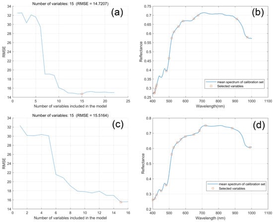
Figure 4.
Feature wavelengths selection by SPA. (a) RMSE trend chart of SG–SPA and the minimum RMSE denoted by red square; (b) feature bands selected by SPA with SG-input; (c) RMSE trend chart of SG–UVE–SPA and the minimum RMSE denoted by red square; and (d) feature bands selected by SPA with SG–UVE input.
CARS also were used to feature band selection based on the preprocessed spectra and variables selected by UVE, as shown in Figure 5. Figure 5a shows the screening process of spectral bands of SG–CARS. Before the sampling time is three, the selected feature bands decrease rapidly and are in the “rough selection” stage. When the sampling times are greater than three, the selected feature bands change slowly and are in the “fine selection” stage. With the increase in sampling times, spectral bands with larger contribution rates are retained, and the number of spectral bands decreases from 472 to 56. Figure 5b shows the change process of RMSECV with the increase in sampling times. For SG–CARS, when the sampling time was 35, the RMSECV value was the minimum, and 56 feature bands were extracted. When the sample number was less than 68, a large amount of irrelevant information was screened out, and the RMSE of the prediction model was decreased. However, when the sample number was greater than 68, a small amount of spectral information related to amylose was also eliminated, resulting in a larger RMSE of the model. It can be seen from Figure 4c that the regression coefficients of 472 full bands change trend with sampling times, and the regression coefficient was also selected when the sampling time was 35. And for SG–UVE–CARS, when RMSECV was minimum, the number of feature wavelengths extracted was 35, which was less than the bands selected by SG–CARS.
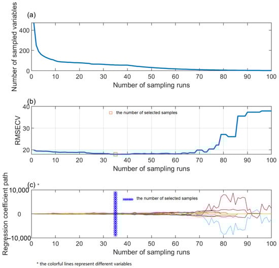
Figure 5.
SG–CARS band selection procedure. (a) the change of the number of sampled variables along with the increase of number of sampling runs; (b) the change of RMSECV along with the increase of the number of sampling runs; (c) the change of regression coefficient along with the increase of the number of sampling runs.
The distribution of the feature bands retained by SG–CARS and SG–UVE–CARS are shown in Figure 6a and b, respectively. Comparing these feature bands, it can be noticed that most of the 35 are also in the 56 feature bands. Amylose has a lot of C–H and some O–H functional groups. Their stretching vibration of the overtones information could be reflected in these feature wavelengths selected. And most of the feature wavelengths are 400–600 nm and 850–950 nm.
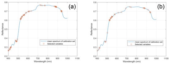
Figure 6.
Distribution of the feature bands selected based on CARS, (a) input with SG pretreated spectra, (b) input with SG–UVE selected.
3.5. PLSR Models
Table 3 shows the results of the PLSR model, which is built from selected characteristic wavelengths. After the prediction model of 15 feature bands selected by SPA, the SPA–PLSR model shows better prediction ability than the full PLSR model, and its Rp reaches 0.890. In the prediction models with 56 and 126 feature bands selected by CARS and UVE algorithms, respectively, the accuracy of the prediction set is even lower than that of the full-band prediction model, which may be due to the elimination of a few feature variables. The Rp of the prediction model established by the UVE algorithm is 0.859, which is better than the accuracy of the model established by the CARS algorithm (Rp = 0.857). Therefore, two models of UVE–CARS–PLSR and UVE–SPA–PLSR are established based on the UVE algorithm. It can be seen that the prediction set accuracy of UVE–CARS–PLSR and UVE–SPA–PLSR models reached 0.888 and 0.868, respectively, which realized the rapid and accurate detection of amylose of lotus seed.
Table 3.
Results of the PLSR model with different extracted characteristic wavelengths.
Figure 7 shows the scatter plots of predicted and measured values of amylose content in the lotus seeds of the SPA–PLSR model. The sample points were closely distributed near the regression line; the Rp was 0.89, the RMSEP was 15.154, and the RPD was 2.19. These results indicate that the model was highly effective in predicting the starch content of lotus seeds with good performance.
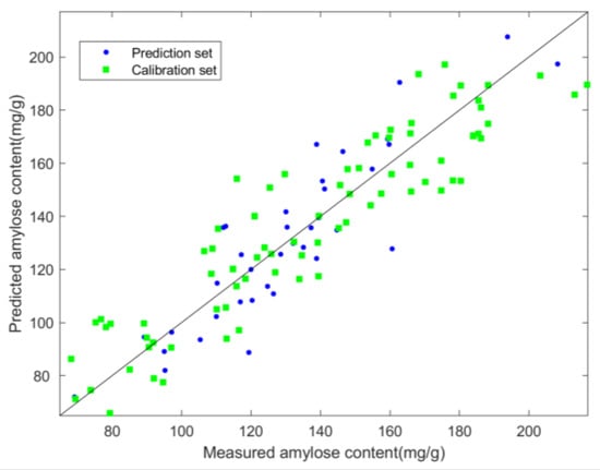
Figure 7.
Scatter plots of predicted versus measured amylose contents obtained from the SPA–PLSR model.
3.6. Visualization of Amylose Content
To facilitate online detection during production, a distribution map of amylose content is useful. To visualize the amylose content, multiple linear regression (MLR) models were established by 15 feature wavelengths selected by SPA to predicate the amylose content of each pixel of the lotus seed. Based on the image and spectra of each pixel in the image, the pseudo-color maps of amylose content were generated. Figure 8 shows some maps and depicts the amylose content in lotus seeds of the three varieties. The color bar indicates a gradual decrease in amylose content from red to blue.
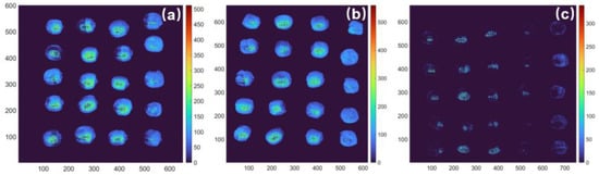
Figure 8.
The distribution maps of the amylose content in lotus seeds of different varieties: (a) Guangchang variety; (b) Jianxuan variety; and (c) Xiang variety.
4. Discussion
This study established different amylose content detection models. All six models could predict the amylose content of lotus seed, and the RMSEP was reduced after feature wavelength selection. The results indicated that either in CARS or UVE–CARS, the Rc and RMSEC are better than other models. Still, Rp and RMSEP did not improve, showing that CARS–PLSR might not be appropriate for this data, as the models exhibited some overfitting. The performance of the UVE-based PLSR model was slightly worse than that of the full-spectra-based PLSR model, possibly because UVE reduced the noise but also eliminated some helpful information. The best prediction model is SPA–PLSR with Rc of 0.916, RMSEC of 15.142/mg g−1, Rp of 0.890, RMSEP of 15.154/mg g−1, and RPD of 2.193, indicating that the SPA algorithm can extract more effective information on characteristic wavelength and has better adaptability to lotus seed spectral data. The RPD > 2.0, which indicated that the model had high reliability and could be used for regression prediction [27]. Only 15 feature wavelengths were used to establish the PLSR prediction model of amylose content in lotus seeds.
In the visualization, it can be seen that the Guangchang and Jianxuan varieties have similar amylose content, with most of the lotus seeds having relatively high content, as shown in Figure 8a,b. However, some lotus seeds in the same variety have significantly lower amylose content, as indicated by the blue pseudo-color of the whole fruit. In contrast, the Xiang variety in Figure 8c shows a significant variation in the amylose content of each lotus seed, with most of the image covered in deep blue, indicating much lower amylose content. These findings are consistent with the measured content of this variety. So, there is a possibility for online detection in lotus seed processing.
5. Conclusions
This work investigates the feasibility of hyperspectral imaging to detect the internal substance in fresh lotus seeds. Hyperspectral images of lotus seeds were obtained for different varieties. A total of 472 spectra variables were reduced into 15 variables by SPA with SG smoothing preprocessed spectra. The PLS models showed promising results, with of 0.916, RMSMEC of 15.142 mg g−1, of 0.890, RMSEP of 15.154, and RPD of 2.193. Based on the selected variables, amylose content distribution maps were also obtained with a satisfactory result. Therefore, the spectra in the vis-NIR range could be considered for the batch evaluation of the amylose content in the lotus seed. The methods developed in this study could serve as a reference for developing online detection equipment.
Author Contributions
Conceptualization, B.Z. and X.W.; methodology, L.H. and S.L.; validation, X.W., D.J. and L.H.; investigation, S.G. and Z.G.; writing—original draft preparation, X.W.; writing—and editing, B.Z.; funding acquisition, X.W. All authors have read and agreed to the published version of the manuscript.
Funding
This research was funded by China Postdoctoral Science Foundation (2019M662216) and interdisciplinary integration to promote the development of intelligent agriculture (horticulture) (000/71202103B).
Data Availability Statement
The data presented in this study are available on request from the corresponding author. The data are not publicly available due to another paper based on that is in preparation.
Conflicts of Interest
The authors declare no conflict of interest.
References
- Sharma, B.R.; Gautam, L.N.S.; Adhikari, D.; Karki, R. A Comprehensive Review on Chemical Profiling of Nelumbo Nucifera: Potential for Drug Development. Phytother. Res. 2017, 31, 3–26. [Google Scholar] [CrossRef]
- Zheng, Y.; Guo, Z.; Zheng, B.; Zeng, S.; Zeng, H. Insight into the Formation Mechanism of Lotus Seed Starch-Lecithin Complexes by Dynamic High-Pressure Homogenization. Food Chem. 2020, 315, 126245. [Google Scholar] [CrossRef] [PubMed]
- Okpala, N.E.; Aloryi, K.D.; An, T.; He, L.; Tang, X. The Roles of Starch Branching Enzymes and Starch Synthase in the Biosynthesis of Amylose in Rice. J. Cereal Sci. 2022, 104, 103393. [Google Scholar] [CrossRef]
- Dhull, S.B.; Chandak, A.; Collins, M.N.; Bangar, S.P.; Chawla, P.; Singh, A. Lotus Seed Starch: A Novel Functional Ingredient with Promising Properties and Applications in Food-A Review. Starch-Starke 2022, 74, 2200064. [Google Scholar] [CrossRef]
- Zheng, M.; Su, H.; You, Q.; Zeng, S.; Zheng, B.; Zhang, Y.; Zeng, H. An Insight into the Retrogradation Behaviors and Molecular Structures of Lotus Seed Starch-Hydrocolloid Blends. Food Chem. 2019, 295, 548–555. [Google Scholar] [CrossRef] [PubMed]
- Sun, H.; Li, J.; Song, H.; Yang, D.; Deng, X.; Liu, J.; Wang, Y.; Ma, J.; Xiong, Y.; Liu, Y.; et al. Comprehensive Analysis of AGPase Genes Uncovers Their Potential Roles in Starch Biosynthesis in Lotus Seed. BMC Plant Biol. 2020, 20, 457. [Google Scholar] [CrossRef]
- Duan, D.X.; Donner, E.; Liu, Q.; Smith, D.C.; Ravenelle, F. Potentiometric Titration for Determination of Amylose Content of Starch—A Comparison with Colorimetric Method. Food Chem. 2012, 130, 1142–1145. [Google Scholar] [CrossRef]
- Fertig, C.C.; Podczeck, F.; Jee, R.D.; Smith, M.R. Feasibility Study for the Rapid Determination of the Amylose Content in Starch by Near-Infrared Spectroscopy. Eur. J. Pharm. Sci. 2004, 21, 155–159. [Google Scholar] [CrossRef]
- Zhang, H.; Miao, Y.; Takahashi, H.; Chen, J.Y. Amylose Analysis of Rice Flour Using Near-Infrared Spectroscopy with Particle Size Compensation. FSTR 2011, 17, 361–367. [Google Scholar] [CrossRef]
- Peiris, K.H.S.; Wu, X.; Bean, S.R.; Perez-Fajardo, M.; Hayes, C.; Yerka, M.K.; Jagadish, S.V.K.; Ostmeyer, T.; Aramouni, F.M.; Tesso, T.; et al. Near Infrared Spectroscopic Evaluation of Starch Properties of Diverse Sorghum Populations. Processes 2021, 9, 1942. [Google Scholar] [CrossRef]
- Özdoğan, G.; Lin, X.; Sun, D.-W. Rapid and Noninvasive Sensory Analyses of Food Products by Hyperspectral Imaging: Recent Application Developments. Trends Food Sci. Technol. 2021, 111, 151–165. [Google Scholar] [CrossRef]
- Wei, X.; He, J.; Zheng, S.; Ye, D. Modeling for SSC and Firmness Detection of Persimmon Based on NIR Hyperspectral Imaging by Sample Partitioning and Variables Selection. Infrared Phys. Technol. 2020, 105, 103099. [Google Scholar] [CrossRef]
- Choi, J.-Y.; Kim, H.-C.; Moon, K.-D. Geographical Origin Discriminant Analysis of Chia Seeds (Salvia Hispanica L.) Using Hyperspectral Imaging. J. Food Compos. Anal. 2021, 101, 103916. [Google Scholar] [CrossRef]
- Tschannerl, J.; Ren, J.; Jack, F.; Krause, J.; Zhao, H.; Huang, W.; Marshall, S. Potential of UV and SWIR Hyperspectral Imaging for Determination of Levels of Phenolic Flavour Compounds in Peated Barley Malt. Food Chem. 2019, 270, 105–112. [Google Scholar] [CrossRef] [PubMed]
- Huang, H.; Hu, X.; Tian, J.; Jiang, X.; Sun, T.; Luo, H.; Huang, D. Rapid and Nondestructive Prediction of Amylose and Amylopectin Contents in Sorghum Based on Hyperspectral Imaging. Food Chem. 2021, 359, 129954. [Google Scholar] [CrossRef] [PubMed]
- Li, S.; Song, Q.; Liu, Y.; Zeng, T.; Liu, S.; Jie, D.; Wei, X. Hyperspectral Imaging-Based Detection of Soluble Solids Content of Loquat from a Small Sample. Postharvest Biol. Technol. 2023, 204, 112454. [Google Scholar] [CrossRef]
- Coliban, R.-M.; Marincaş, M.; Hatfaludi, C.; Ivanovici, M. Linear and Non-Linear Models for Remotely-Sensed Hyperspectral Image Visualization. Remote Sens. 2020, 12, 2479. [Google Scholar] [CrossRef]
- ElMasry, G.; Wang, N.; ElSayed, A.; Ngadi, M. Hyperspectral Imaging for Nondestructive Determination of Some Quality Attributes for Strawberry. J. Food Eng. 2007, 81, 98–107. [Google Scholar] [CrossRef]
- Yang, Z.; Xiao, H.; Zhang, L.; Feng, D.; Zhang, F.; Jiang, M.; Sui, Q.; Jia, L. Fast Determination of Oxide Content in Cement Raw Meal Using NIR Spectroscopy with the SPXY Algorithm. Anal. Methods 2019, 11, 3936–3942. [Google Scholar] [CrossRef]
- Rinnan, A.; van den Berg, F.; Engelsen, S.B. Review of the Most Common Pre-Processing Techniques for near-Infrared Spectra. Trends Anal. Chem. 2009, 28, 1201–1222. [Google Scholar] [CrossRef]
- Wu, D.; Sun, D.-W. Advanced Applications of Hyperspectral Imaging Technology for Food Quality and Safety Analysis and Assessment: A Review—Part I: Fundamentals. Innov. Food Sci. Emerg. Technol. 2013, 19, 1–14. [Google Scholar] [CrossRef]
- Centner, V.; Massart, D.L.; de Noord, O.E.; de Jong, S.; Vandeginste, B.M.; Sterna, C. Elimination of Uninformative Variables for Multivariate Calibration. Anal Chem 1996, 68, 3851–3858. [Google Scholar] [CrossRef] [PubMed]
- Xu, J.-L.; Esquerre, C.; Sun, D.-W. Methods for Performing Dimensionality Reduction in Hyperspectral Image Classification. J. Near Infrared Spectrosc. 2018, 26, 61–75. [Google Scholar] [CrossRef]
- Li, H.; Liang, Y.; Xu, Q.; Cao, D. Key Wavelengths Screening Using Competitive Adaptive Reweighted Sampling Method for Multivariate Calibration. Anal. Chim. Acta 2009, 648, 77–84. [Google Scholar] [CrossRef] [PubMed]
- Zhang, C.; Liu, F.; Kong, W.W.; Cui, P.; He, Y.; Zhou, W.J. Estimation and Visualization of Soluble Sugar Content in Oilseed Rape Leaves Using Hyperspectral Imaging. Trans. ASABE 2016, 59, 1499–1505. [Google Scholar] [CrossRef]
- Jie, D.; Xie, L.; Rao, X.; Ying, Y. Using Visible and near Infrared Diffuse Transmittance Technique to Predict Soluble Solids Content of Watermelon in an On-Line Detection System. Postharvest Biol. Technol. 2014, 90, 1–6. [Google Scholar] [CrossRef]
- Tamaki, Y.; Mazza, G. Rapid Determination of Carbohydrates, Ash, and Extractives Contents of Straw Using Attenuated Total Reflectance Fourier Transform Mid-Infrared Spectroscopy. J. Agric. Food Chem. 2011, 59, 6346–6352. [Google Scholar] [CrossRef] [PubMed]
Disclaimer/Publisher’s Note: The statements, opinions and data contained in all publications are solely those of the individual author(s) and contributor(s) and not of MDPI and/or the editor(s). MDPI and/or the editor(s) disclaim responsibility for any injury to people or property resulting from any ideas, methods, instructions or products referred to in the content. |
© 2023 by the authors. Licensee MDPI, Basel, Switzerland. This article is an open access article distributed under the terms and conditions of the Creative Commons Attribution (CC BY) license (https://creativecommons.org/licenses/by/4.0/).