CLT-YOLOX: Improved YOLOX Based on Cross-Layer Transformer for Object Detection Method Regarding Insect Pest

Abstract

This paper presents an enhanced YOLOX-based algorithm for pest detection, adopting a nature-inspired approach for refining its methodology. To tackle the limited availability of image data pertaining to pests and diseases, the paper incorporates Mosaic and Mixup technologies for effective image preprocessing. Furthermore, a novel training strategy is proposed to enhance the overall quality of the results. The existing architecture is enriched by integrating shallow information, while the CLT module is devised to facilitate cross-layer fusion and extract essential feature information. This advancement enables improved object detection across various scales. Additionally, the paper optimizes the original PFPN structure by eliminating the convolutional layer preceding upsampling, enhancing the C3 module, and integrating the convolutional attention model (CBAM) to identify salient regions within complex scenes. The performance of the proposed CLT-YOLOX model is extensively evaluated using the IP102 dataset, demonstrating its effectiveness. Notably, the model exhibits significant improvements compared to the original AP evaluation index, with an increase of 2.2% in average precision (mAP) and 1.8% in AP₇₅. Furthermore, favorable results are achieved in the COCOmAP index, particularly in the AP_small category where there is a 2.2% improvement in performance.

1. Introduction

In China, being a major agricultural nation, integrated pest management is crucial for sustainable agricultural development. Every year, the presence of diverse pests poses significant challenges during crop cultivation, resulting in reduced crop yields and compromised quality. In severe cases, these challenges can lead to widespread crop failures. In addition, many pests are very similar; for example, Lepidoptera contains dozens of common field crop pests, and their physical characteristics are very similar, and secondly, the size of the pests is different, and some pests will be small enough to distinguish morphology in photos. What is more complicated is that each pest may be at different in-sect ages and developmental stages, such as the larval stage and adult stage, resulting in the appearance of even the same pest being very different, which causes the field “pest detection” need to detect multi-posture, multi-species, multi-form pests, bringing much greater technical challenges than other detection recognition. Therefore, the accurate and effective classification and identification of insects are essential for implementing timely pest control measures and mitigating substantial economic losses in crop production.

Traditional approaches to classify and identify diseases and insect pests heavily depend on the expertise of insect specialists or taxonomists who accumulate research experience through professional knowledge and literature references. However, this method is slow, inefficient, costly, subjective, and often lacks timeliness. Even with extensive knowledge and experience, it remains challenging to avoid species confusion. The continuous advancement of the Internet and information technology has introduced new methods and ideas for crop disease and insect pest identification. Efficient image recognition technology has emerged as a solution to improve recognition efficiency, reduce costs, and enhance accuracy. Various operators such as SIFT [1], LBP [2], ORB [3], and SURF [4] have been employed to represent targets. Machine learning techniques like Support Vector Machine (SVM) [5], k-Nearest Neighbors (KNN) [6], and Random Forest [7] are then utilized for target recognition. However, these feature-based methods heavily rely on the representation of feature operators and are not robust against illumination variations, occlusion, complex environments, and interference from similar targets.

With the rapid development of deep learning technology, researchers have increasingly applied it to image recognition, leading to significant advancements in recent years. Deep learning is characterized by its complex network structures and the ability to handle large-scale datasets, which are key features of this technology. The emergence of deep learning has provided a robust technical foundation for image recognition tasks. Various deep learning models, including Deep Belief Network (DBN) [8], convolutional neural network (CNN) [9], Recurrent Neural Network (RNN) [10], Generative Adversarial Network (GAN) [11], Capsule Network (CapsNet) [12], and more, have been proposed. However, it is challenging for these methods to fully meet practical requirements, and many of them are primarily limited to laboratory-level research.

In recent years, computer vision technology applied in the field of agricultural engineering, specifically utilizing deep learning algorithms, has gained increasing attention and favor from experts and scholars worldwide. Compared to traditional machine vision techniques, deep-learning-based computer vision offers a superior efficiency and accuracy in various areas, including image processing, feature extraction, feature abstraction, and feature classification. As a result, numerous pest identification and classification methods based on deep learning have been proposed. These advancements aim to enhance and address the limitations of current pest identification methods, ultimately achieving more timely and effective pest control measures.

In 2016, Wu Xiang from Zhejiang University [13] successfully applied a convolutional neural network (CNN) model to identify 10 species of moth pests, such as box borer, corn borer, rice leaf roller, mole cricket, and others. The image dataset consisted of 900 color images collected from the natural environment, with each image containing a single pest. The CNN pest recognition model comprised five layers, achieving a recognition accuracy of approximately 76.7%. Wang et al. [14] proposed a plant pest recognition method based on a CNN with initial modules and extended convolutions. Huang et al. [15] developed a CNN model to classify eight types of tomato pests and employed transfer learning to reduce training time. However, these approaches are limited by their small dataset, which may result in knowledge limitations and overfitting during the model learning. Moreover, the extracted features are relatively simplistic, leading to inadequate generalization capabilities in real-world scenarios.

Thanks to the progress in deep learning technology, numerous detectors based on convolutional neural networks have achieved an impressive detection performance. Single-stage detectors [14] directly employ convolutional neural networks to predict the category and location of targets. Alternatively, Faster R-CNN [16] generates region proposals through a region proposal network, enabling more accurate classification and regression tasks. As well as the plug-and-play module [17] applied to the R-CNN model that has just been proposed in recent years, they designed a module to create a query-based model to be able to reason about different numbers of suggestions, and further extended it to a dynamic model. However, whether it can be applied to the YOLO series target detection, the answer is not given in the article. Transformer-based detectors [18,19], on the other hand, eliminate the need for Anchor constraints and post-processing steps like non-maximum suppression. This end-to-end implementation simplifies the object detection pipeline significantly.

In the domain of target detection, the YOLO series [20,21] has played a significant role as a standalone detector. For example, Cai et al. [22] proposed an improved YOLOv4 target detection framework applied to the algorithm of self-driving cars, which improves the detection accuracy and supports real real-time detection operations. Compared with the original model, it shows a higher average accuracy and inference speed. This paper introduces an enhanced model called CLT-YOLOX, based on YOLOX [23], to address the aforementioned challenges. Figure 1 provides an overview of the detection pipeline in CLT-YOLOX, which incorporates data augmentation during training. This approach expands the dataset and enhances adaptability to significant variations in object sizes within images. To effectively combat overfitting during training, a data augmentation strategy is proposed. The backbone of CLT-YOLOX utilizes the CSPDarknet [24] network, following the original version. Before the input of the original small detection head, a special CLT module is introduced, which processes tiny objects by fusing feature information extracted from different scales. In a Path Aggregation Network (PANet) [25], we achieve direct upsampling by removing the convolution operation in the upsampling stage. Furthermore, improvements are made to the C3 module in PFPN. Compared to BIFPN [26], our method is similar in that it chooses to delete nodes with only one input edge, and we choose to delete the convolution operation before upsampling to save on computational cost. Furthermore, to capture attention in images with a significant coverage, we incorporate the Convolutional Attention Module (CBAM) [27]. As a result, our enhanced CLT-YOLOX model demonstrates a superior performance in handling agricultural pest images compared to YOLOX.

Our contributions are summarized as follows:

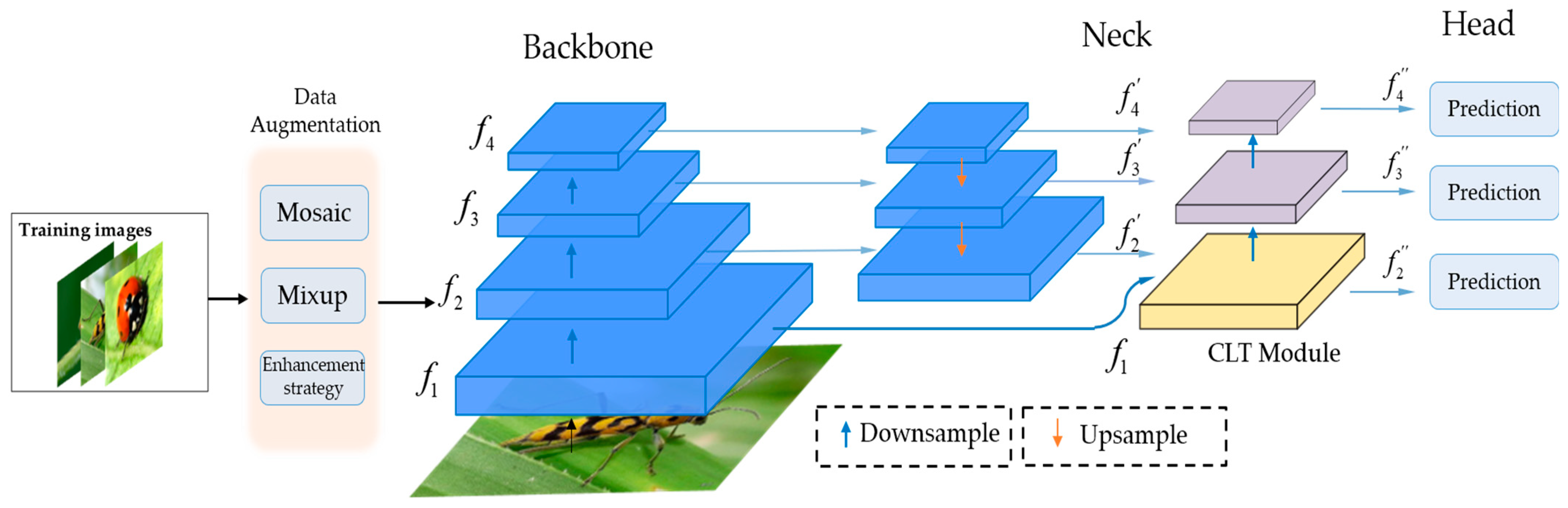
• Addressing the scarcity of real pest image data: To overcome the limited availability of real pest image data in the field, we employed Mosaic and Mixup data augmentation techniques. These techniques effectively augment the dataset, allowing for a better model generalization. Additionally, a novel data enhancement strategy was introduced to further improve the model’s performance.
• Cross-Layer Transformer (CLT) module: Our proposed CLT (Cross-Layer Transformer) module incorporates cross-layer information, enabling the extraction of fine-grained features more effectively. By leveraging this cross-layer information, our model achieves improved detection results compared to the original YOLOX algorithm.
• Enhancements to the C3 module and integration of CBAM: We enhanced the C3 module within the PFPN structure by removing the convolution operation before the upsampling stage. Additionally, we integrated the Convolutional Block Attention Module (CBAM) to capture attention in complex scenes. These modifications enhance the recognition ability for multi-scale targets while managing the trade-off between computational requirements and accuracy.
• Performance improvements: The improved YOLOX algorithm proposed in this paper achieved an average precision (AP) of 57.7% on the public IP102 dataset. This performance is 2.2% higher than the original YOLOX model. Notably, the AP_small value increased by 2.2%, demonstrating the effectiveness of our enhancements in detecting small targets.

2. Related Work

2.1. Data Augmentation

Data augmentation is an invaluable technique that expands the dataset and enhances the model’s robustness across various scenarios. Commonly used methods for global pixel-level augmentation include random scaling, cropping, translation, shearing, and rotation. These techniques introduce variations in the training images, allowing the model to learn to be invariant to different transformations.

In addition to these standard augmentation methods, researchers have introduced advanced techniques that involve combining multiple images to further augment the dataset. Two notable techniques are Mosaic [24] and Mixup [28].

Mosaic, an improvement over Cutmix [29], combines four images to create a single augmented image. This technique effectively enriches the dataset by introducing diverse backgrounds and objects within a single image. By incorporating random scaling, Mosaic introduces a wider range of small targets, which enhances the network’s ability to detect and classify them accurately. The Mosaic technique has proven to be effective in improving the model’s robustness and generalization performance.

Mixup is another powerful data augmentation technique that enhances the diversity of the dataset. It randomly selects two training samples and performs a weighted summation of their pixel values, as well as their corresponding labels. This process generates new training samples that lie along the line connecting the original samples in the input space. By blending samples together, Mixup encourages the model to learn from the interpolated samples, effectively regularizing the model and reducing overfitting. Mixup has been shown to improve the model’s performance, particularly in scenarios with limited training data.

Both Mosaic and Mixup techniques significantly enhance the dataset’s diversity and quality, leading to notable improvements in the model’s performance. By incorporating these advanced data augmentation techniques, our model becomes more robust and capable of handling variations in real-world scenarios.

2.2. Pest Identification

Pest identification has undergone various advancements with the emergence of new technologies. In the early stages, pest detection relied on traditional machine learning approaches, typically involving two steps: feature extraction and model training. Feature extraction aimed to extract significant and relevant features, such as shape, texture, or color, from pest images to represent the target. For instance, Hassan et al. [30] developed an intelligent insect classification system that utilized shape and color features to identify locusts and butterflies. The use of Histogram of Oriented Gradient (HOG) features initially gained attention in pedestrian detection [31] and was later applied to insect detection by Shen et al. [32]. Rani et al. [33] employed an SVM classifier to identify whiteflies, aphids, and thrips in leaf images. While traditional machine learning approaches achieved certain success in specific scenarios, they heavily relied on manual feature extraction, lacked robustness, and exhibited limited generalization ability. Consequently, they struggled to adapt to scene variations and migration.

In contrast, deep learning has gained significant popularity in recent years. It leverages convolutional neural networks (CNNs) to automatically extract features from data, enabling end-to-end training. Deep learning models exhibit lightweight architectures and strong generalization capabilities, delivering an impressive performance in subsidiary tasks like target tracking and image recognition.

For instance, Chen et al. [34] developed a new CNN model for pest recognition, building upon traditional CNNs. They evaluated their model on a dataset of 550 images across 10 categories in natural backgrounds, achieving an accuracy rate of approximately 99.67%. CNN-based target detection models can be categorized into different types: Anchor-based detectors, such as Scaled YOLOv3 [20], YOLOv4 [24], and YOLOv5 [21]. Researchers like HE et al. [35] have employed deep learning techniques, improving upon Fast R-CNN and YOLOv3 models, to develop pest detection models for specific pests like brown rice planthoppers, resulting in an enhanced pest recognition accuracy. There are also Anchor-free detectors, including CenterNet [36], YOLOX [23], and RepPoints [37]. For example, Huang et al. [38] proposed a forest pest detection algorithm based on YOLOX. They introduced a bidirectional cross-scale feature fusion mechanism in the network architecture, achieving favorable results. Typically, these detectors consist of two main components: a CNN-based backbone for image feature extraction and a detection head responsible for predicting object categories and bounding boxes. Moreover, recent object detectors often incorporate additional layers inserted between the backbone and the detection head, commonly referred to as the “neck” of the detector.

Recently, Transformers have utilized multi-head attention to extract a feature with long-range dependencies. For example, based on the yolov5 model, Zhao et al. [39] proposed a cross-layer asymmetric Transformer (CA-Trans), which is designed to replace additional prediction heads, and proposed a sparse local attention (SLA) module with additional asymmetric information between heads. Good results have been achieved in drone image datasets. Another example is Zhang et al. [40]’s proposal of a Cross-Layer Aggregation with Transformers (CAT) framework, which leverages Transformers to capture the long-range dependencies of CNN-based features with the long-range dependencies module and aggregate the features layer by layer with the cross-layer fusion module. Inspired by the attention principle of Transformer and CoTNet, the CLT module proposed in this paper combines the ability of Transformer to capture global information with the ability of CNN to capture nearby local information. Instead of using the traditional Transformer module to embed the module in position, the CNN structure is used to obtain local location information. The amount of computation and the number of arguments are reduced by using group convolution. The CLT module combines asymmetric feature information extracted from different layers to enrich the features of the detection head.

In CLT-YOLOX, our focus lies in improving the “neck” part of the model. We aim to enhance the feature fusion and information extraction capabilities within this component. By leveraging cross-layer information and incorporating advanced techniques, our CLT-YOLOX model achieves an improved performance in pest identification tasks.

3. Materials and Methods

To overcome the limitations of existing pest detection methods, such as small datasets and simplistic feature extraction, YOLOX is recognized as one of the most accurate object detectors, offering a competitive inference speed, and introducing enhanced data augmentation techniques for data preprocessing. It employs an Anchor-free framework, effectively addressing the class imbalance issue commonly encountered in Anchor-based methods. Additionally, YOLOX uses decoupled heads to handle classification and regression tasks separately, and the recent trend of detection models is to use decoupled heads instead of original detection heads, which helps to improve the accuracy and efficiency of object detection tasks. We adopt the YOLOX [21] framework to enhance the effectiveness of pest detection. The YOLOX series consists of six models: YOLOX-Nano, YOLOX-Tiny, YOLOX-S, YOLOX-M, YOLOX-L, and YOLOX-X. Compared to YOLOX-M, which has 25.3M parameters, YOLOX-S has only 9.0M parameters, making it a smaller and more suitable option for future deployment on handheld devices. While YOLOX-Tiny and YOLOX-Nano utilize depth-wise convolution to further reduce the number of parameters, they do sacrifice some accuracy, particularly in the AP_small index. As a result, we have chosen YOLOX-S as the benchmark model due to its relatively smaller parameter size while still maintaining an acceptable accuracy for pest image recognition tasks.

To address the scarcity of real pest images, we employ the Mosaic and Mixup techniques to process the training data. These data augmentation methods significantly enhance the dataset’s diversity and quality. Additionally, we propose a new enhancement strategy to further improve the model’s performance.

To extract fine-grained features, we introduce shallow information into the existing network architecture. We propose the CLT module, which incorporates cross-layer information fusion, to effectively extract features. Furthermore, we enhance the feature pyramid structure and strike a balance between data volume and accuracy. The overall framework of our algorithm is depicted in Figure 2.

3.1. Data Enhancement

In this paper, two fundamental data augmentation techniques, Mosaic and Mixup, are employed. Mosaic data augmentation: By applying a series of random operations to four images, the background of the detected objects in the dataset is significantly enriched. This technique enhances the diversity of the training data and improves the model’s ability to handle complex backgrounds. Mixup: Randomly selecting two images from the training dataset, the samples are combined through a weighted summation, and the labels of the samples are also weighted accordingly. This process helps to reduce the impact of incorrect labels and enhances the model’s robustness. The impact of data augmentation is illustrated in Figure 3.

3.2. Backbone

The backbone of the CLT-YOLOX architecture utilizes the CSPDarknet [24] module for feature extraction, aiming to maximize the gradient divergence. To prevent redundant gradient information from different layers, the gradient flow truncation method is employed. This approach enhances the feature extraction capability of the convolutional network, resulting in an improved detection speed and reduced computational overhead, all while maintaining a high detection accuracy. When compared to other commonly used backbone networks, the CSPDarknet module demonstrates a superior performance in feature extraction without compromising detection accuracy, leading to an improved efficiency and reduced computational cost.

To facilitate a more detailed discussion, let us define the model structure in mathematical terms. We will denote the input image as x, then $f_0=Focus\left(x\right)$, and the four feature outputs of the backbone network can be expressed as i = 1, …, 4. These four features in Formula (1) produce the following:

$$\begin{array}{c}{f}_i=B_i\left(f_{i-1}\right),i=1,\dots ,4\end{array}$$

(1)

The backbone network is defined by different regions denoted as $B_i\left(·\right)$. These regions include blocks $B_1\left(·\right)$, $B_2\left(·\right)$, and $B_3\left(·\right)$, which consist of a convolutional layer (Conv) followed by 3 or 9 CSPBottleneck modules. Additionally, there is a region $B_4\left(·\right)$, which is composed of a Conv layer, 3 CSPBottleneck modules, and an SPP (Spatial Pyramid Pooling) module. Each module is described as follows:

• Focus module: The focus module slices an image by taking a value for each pixel at an interval (similar to adjacent down sampling). This process integrates information from the width (W) and height (H) dimensions into the channel space. The output channel is expanded by four times, resulting in a spliced image with 12 channels. This increase in channels benefits subsequent calculations. Figure 4 illustrates the concept of the focus module.
• SPP module: The SPP module is inspired by the idea of Spatial Pyramid Pooling. It utilizes a pooling layer composed of three convolutional kernels with different sizes (5 × 5, 9 × 9, 13 × 13) to fuse local features and global features. This enriches the expression capability of the final feature map. The SPP module enhances the network’s ability to capture features at different scales, improving the overall performance. Figure 4 provides an illustration of the SPP module.

These modules, including the focus module and the SPP module, play a crucial role in the backbone network of CLT-YOLOX. They enable effective feature extraction and information integration, contributing to the accurate detection of objects in the subsequent stages of the architecture.

3.3. Improved Neck

3.3.1. Improved C3 Module

In the CLT-YOLOX architecture, the C3 module, responsible for feature fusion and extraction, is improved to enhance the model’s ability to extract and distinguish important information specific to each pest species in the image. The improved version is called the C2F module, which combines the C3 module from the original model with the ELAN (Efficient Lightweight Attention Network) [40] concept.

The original C3 module in YOLOX utilized the CSPNet [41] (Cross-Stage Partial Network) to introduce the concept of splitting and incorporated a residual structure. The C2F module in this paper builds upon the C3 module and integrates the ELAN idea to achieve a light weight while capturing a broader range of gradient flow information. The C2F module enhances the ability of the model to learn and represent complex patterns in pest images. Figure 5 shows the respective structure of the C3 module and C2F in detail.

3.3.2. Convolutional Block Attention Module (CBAM)

The CLT-YOLOX model incorporates the CBAM (Convolutional Block Attention Module) [22] to enhance its ability to capture attention regions in pest images. CBAM is a lightweight attention module known for its simplicity and effectiveness in improving feature representation. It seamlessly integrates into CNN architectures and can be trained end-to-end.

The CBAM module operates on a feature map and sequentially derives attention maps along two independent dimensions: channel and spatial. The channel attention mechanism captures interdependencies between channels, allowing the model to focus on informative channels while suppressing less relevant ones. The spatial attention mechanism highlights spatial regions of interest by modelling interdependencies between spatial locations. These attention maps are then multiplied with the input feature map, enabling adaptive feature refinement. Its structure is shown in Figure 6.

3.3.3. Cross-Layer Transformers Module

There are also four features in the “neck”, where $f_1$ directly enters the new module, so in the expression of $f_i^{\prime }$, i = 2, …, 4. These three features can be expressed as follows:

$$\begin{array}{c}{f}_i^{\prime }=\left\{\begin{array}{c}{N}_i\left(f_i ,f_{i+1}^{\prime }\right),i=2,3 \\ f_{i },i=4\end{array}\right. \end{array}$$

(2)

In the formula, the expression of $N_i\left(·,·\right)$ is as follows:

$$\begin{array}{c}{N}_i\left(f_i, f_{i+1}^{\prime }\right)=UB(Cat\left(f_i ,US\left(f_{i+1}^{\prime }\right)\right) \end{array}$$

(3)

Among them, $Cat\left(·,·\right)$ represents a connection operation, $US\left(·,·\right)$ represents an upsampling operation, and $UB\left(·\right)$ represents a combination of different modules. In Formula (3), the index i starts at 2. In $N_2\left(·,·\right)$ and $N_3\left(·,·\right)$, $US\left(·\right)$ consists of three C2F modules and one CBAM module.

We define the features before the last three convolutional layers as $f_i^{″}$ where i = 2, …, 4. So, we obtain Formula (4):

$$\begin{array}{c}{f}_i^{″}=H_i\left(f_i^{\prime } ,f_{i-1}^{″}\right),i=2,3,4\end{array}$$

(4)

where $H_i\left(·,·\right)$ represents a different block, similar to $N_i\left(·,·\right)$.

$$\begin{array}{c}{H}_i\left(f_i^{\prime }, f_{i-1}^{″}\right)=\left\{\begin{array}{c}DB(Cat\left(f_i^{\prime }, Conv\left(f_{i-1}^{″}\right)\right),i=2,3\\ C2F(Cat\left(f_i^{\prime },Conv\left(f_{i-1}^{″}\right)\right),i=4\end{array}\right. \end{array}$$

(5)

$DB\left(·\right)$ also represents different blocks, and $DB\left(·\right)$ in $H_2\left(·,·\right)$ and $H_3\left(·,·\right)$ are composed of one CBAM module and three C2F modules, respectively. In $H_4\left(·,·\right)$, the CBAM operation is omitted and the direct output is selected After obtaining $f_i^{\prime \prime }$, we can obtain the final prediction as shown in Equation (6):

$$\begin{array}{c}{P}_i=Conv\left(f_i^{\prime \prime }\right), i=2,3,4\end{array}$$

(6)

where $P_i$ represents three output predictions from different prediction heads.

Inspired by CoTNet [42], this paper proposes a multi-scale fusion algorithm that combines the output of the backbone network $f_1$, $f_2$, $f_3$, $f_4$. In order to better extract fine-grained features, this paper proposes the algorithm CLT in the “neck” part. Considering the shallow information of the original framework, $f_1$ is further introduced so that the small path $f_1$ and the small path $f_2^{\prime }$ are introduced into the CLT module as keys, and the query and value, respectively, to predict the final $f_2^{\prime \prime }$. The cross-layer feature Transformer is then realized. The new $P_2$, as Formula (7), is as shown:

$$\begin{array}{c}{P}_2=Conv\left(Cat\left(CLT\left(f_1,f_2^{\prime }\right),f_2^{\prime }\right)\right)\end{array}$$

(7)

The CLT module is utilized as a cross-layer feature Transformer. To fuse and extract feature information from different output sizes, we designed the CLT module as depicted in the figure. It takes inputs $f_1$ and $f_2^{\prime }$ and generates output $f_2^{\prime }$. Additionally, K and Q are generated from $f_1$, while V is generated from $f_2^{\prime }$. In this context, $f_1\in R^{2H\times 2W\times C}$, $f_2^{\prime }\in R^{H\times W\times 2C}$.

Next, let us delve into the detailed steps of the CLT module. The flowchart is shown in Figure 7. Initially, we consider $K^1=Conv\left(f_1\right)$ as the static representation of the input. Instead of using a 1 × 1 convolution, we spatially align all adjacent keys within the k × k grid and perform a k × k group convolution. This process enables the learned contextualized keys to inherently capture the static key information from neighboring keys. Subsequently, the connection operation is executed, as illustrated in Formula (8).

$$\begin{array}{c}{Y}^1=Cat\left(K^1,f_1\right)\end{array}$$

(8)

where $Cat\left(·,·\right)$ represents the connection operation; after the connection operation, two different convolution operations are performed to obtain the attention matrix A, as shown in Formula (9):

$$\begin{array}{c}A=\left[Y^1\right] W_{\theta }{W}_{\delta }\end{array}$$

(9)

where $\theta$ and $\delta$ represent two consecutive 1 × 1 convolution operations ($\theta$ with the activation function and $\delta$ without the activation function).

Next, we will process another input $f_2^{\prime }$ in the CLT module. Firstly, we apply a convolution operation on $f_2^{\prime }$, denoted as $V^1=Conv\left(f_2^{\prime }\right)$. Then, $Conv\left(·\right)$ represents a 1 × 1 convolution operation, which adjusts the number of channels for the subsequent fusion process. As a result, the dimension of $V^1$ is transformed to $V^1\in R^{HW\times 2C}$.

In other words, for each head, the local attention matrix of $A$ at each spatial position is learned based on the query feature, incorporating more realistic key features that are contextually relevant. This approach enhances the self-attention learning with the additional guidance from the static context $K^1$. Subsequently, we obtain the feature map $V^1$ by combining the participation of $f_2^{\prime }$. The details are shown in Figure 8. Finally, we obtain the resulting feature map $K^2$.

$$\begin{array}{c}{K}^2=softmax\left(A\right)\otimes V^1\end{array}$$

(10)

To ensure compatibility with the feature map $K^2$, a convolution operation is applied to $K^1$, adjusting its size to match that of $K^2$. The final output of the CLT module is the concatenation $K_{out}$ of the dynamic feature map $K^2$ and the stastic feature map $K^1$, which captures the dynamic feature interaction between inputs from different feature layers.

$$\begin{array}{c}{F}_{out}=K^1+K^2\end{array}$$

(11)

The entire workflow of CLT can be seen in Algorithm 1.

Algorithm 1: Cross-Layer Transformer

Input: input feature maps, Q, K, V

$f_1$←K, Q, $f_2^{\prime }$←V

Output: output Fout

1.   Set kernel_size = 3, stride = 2$, f_1.shape$ = c, 2h, 2w$, f_2^{\prime }.shape$ = 2c, h, w 2.   $K^1\leftarrow \mathrm{KeyConv} \left(f_1\right)$ (padding = kernel_size/2, group = 4) 3.   $V^1\leftarrow \mathrm{ValueConv} \left(f_2^{\prime }\right)$ 4.   $Y^1\leftarrow \mathrm{Concat} (K^1, f_1, \dim = 1)$ 5.   $\mathrm{A}\leftarrow \mathrm{AttenConv} \left(Y^1\right) (W_{\theta }\leftarrow \mathrm{Conv} \mathrm{with} \mathrm{Relu}, W_{\delta }\leftarrow \mathrm{Conv} \mathrm{without} \mathrm{Relu})$ 6.   Change the size of matrix A to (2c, 2 × 2, h, w) 7.   Average matrix A over dimension 2 8.   A.Mean (2, keepdim = False). View(2c, −1) 9.   K2← softmax (A, dim = 1) ∗ V1 10. K1← Conv (kernel_size, stride) 11. Change the size of matrix K2 to (2c, h, w) 12. $F_{out}\leftarrow K^1+K^2$ 13. return $F_{out}$

3.4. Head

As depicted in Figure 2, the head section comprises three prediction heads, each consisting of separate classification and regression branches. These branches are concatenated along the channel dimension, and a reshape operation is applied by multiplying the width (W) and height (H). Subsequently, the three prediction heads are concatenated along the W × H dimension, and the loss is calculated based on this combined output.

3.4.1. Decoupled Head

In previous versions of the YOLO series, the regression task and the classification task shared the parameters of the preceding layer, which may not have been optimal for both tasks. To address this, the proposed model divides the vector input to the head into two parts, specifically for detection box regression and target classification. This division allows the classification task to focus more on determining which extracted features are most relevant to the existing categories, while enabling the regression task to prioritize the position coordinates and correct the bounding box parameters more accurately. This approach accelerates the convergence speed of the model and enhances detection accuracy.

3.4.2. Anchor Free

Currently, there are two mainstream methods for object detection: Anchor-based and Anchor-free. For instance, YOLOv3 and YOLOv5 employ the Anchor-based method to extract target frames and compare them with annotated ground truth frames to assess the differences. In contrast, this model utilizes the Anchor-free method to overcome the limitations of the Anchor-based approach. It directly predicts four numerical values at each position on the output feature map, which determine the offsets of the top-left and bottom-right corners relative to the target at that particular position. This approach eliminates the need for predefined Anchor boxes and allows for more flexibility in detecting objects of various sizes and aspect ratios.

3.4.3. SimOTA

The traditional distribution method of positive samples is inappropriate. The function of SimOTA proposed in this model is to set different numbers of positive samples for different targets. The formula is as follows:

$$\begin{array}{c}{c}_{ij}=L_{ij}^{cls}+\lambda L_{ij}^{reg}\end{array}$$

(12)

In the equation, $\lambda$ represents the balance coefficient, cls represents the category loss between the Anchor box and the predicted value, and reg represents the regression loss between the Anchor box and the predicted value. During the training process, each Anchor box undergoes adaptive adjustment within a fixed central area. The algorithm dynamically allocates k positive samples and assigns positive labels to the corresponding grid cells for these positive predictions, while the remaining grid cells are labeled as negative. Compared to OTA (Online Training Algorithm), SimOTA (Simple Online Training Algorithm) significantly reduces training time and computational complexity.

3.4.4. Loss Function

We calculate the classification loss and regression loss using Binary cross entropy, which is as follows:

$$\begin{array}{c}BCELoss=-\left(\mathrm{ylog}\left(\mathrm{p}\left(\mathrm{x}\right)\right)+\left(1-\mathrm{y}\right)\log \left(1-\mathrm{p}\left(\mathrm{x}\right)\right)\right)\end{array}$$

(13)

Among the above, y represents the Binary label—the value is 0 or 1—and $\mathrm{P}\left(\mathrm{x}\right)$ is the probability of predicting each category.

4. Experiments

4.1. Implementation Details

4.1.1. Datasets

The dataset selected for this experiment is IP102 (a large-scale benchmark dataset for pest identification). This dataset has 102 categories and contains 18,981 pictures. These images contain backgrounds that are directly fed into the data enhancement part of the model during the training phase, as shown in Figure 3. The dataset was randomly di-vided into a training set and a test set, with a ratio of 7:3. One-third of the test set was used for training process validation, resulting in 13,283 instances being used for training. The validation set and test set consisted of 1897 and 3796 instances, respectively, which were used to evaluate the model’s performance. The dataset distribution is shown in Figure 9:

4.1.2. Experimental Environment

In the experiment, Python3.8.15 and Pytorch1.12.0 were used. The graphics card model is 3090, and the version is CUDA11.6.

4.1.3. Network Parameter

In our experiment, the YOLOX_s model with fewer parameters is used, and the pre-training weight is obtained from the official training dataset of COCO-Train2017, specifically yolox_s.pth. The improved model shares most of the backbone and some parts of the head with the original model. By utilizing these pre-trained weights, a significant amount of training time can be saved.

Since the main focus of this experiment lies in the “neck” part, the pre-training weights of the backbone network are considered universal. To facilitate better learning in the “neck” part, the frozen training method is employed in the initial stage of the experiment. The first 50 epochs are dedicated to frozen training, during which the weights of the backbone network remain frozen. This allows the feature extraction network to remain unchanged while fine-tuning the network. This approach helps the “neck” part capture more informative features before engaging in the overall model training, ultimately accelerating the convergence time of the model.

After the frozen training phase, the model undergoes approximately 100 epochs of training to achieve the best results. Therefore, the total number of training epochs is set to 150. The learning rate is initialized to 0.01, the learning rate is set to $lr=lr\times Batch\_Size/64$, and the learning rate adjustment adopts the cosine annealing strategy. The batch size during frozen training is set to 32, while the batch size during unfrozen training is reduced to 16. The minimum learning rate is determined as the initial learning rate multiplied by 0.01.

In this experiment, a new data augmentation strategy is proposed to improve the results. Following the official recommendation of YOLOX, the augmentation level is adjusted based on the model size and dataset size. For small models, the augmentation is weakened, while for large models or small datasets, augmentation is enhanced.

The experiment incorporates several data augmentation techniques to achieve a better performance. Firstly, the Mosaic augmentation probability (mosaic_prob) is set to 0.5. This means that there is a 50% chance that the input image will be enhanced using Mosaic augmentation. Additionally, the Mixup augmentation probability (mixup_prob) is set to 0.5. Consequently, there is a 50% chance of applying Mixup augmentation after Mosaic augmentation. Therefore, the overall probability of using Mixup augmentation is calculated as mosaic_prob × mixup_prob, which results in a 25% probability of using Mixup augmentation in this experiment.

Furthermore, inspired by YOLOX, it is recognized that the training images generated with Mosaic augmentation may deviate from the distribution of natural images. To address this, when Mosaic augmentation is enabled (mosaic = True), a separate parameter called special_aug_ratio is set. This parameter allows Mosaic augmentation to be enabled within a specific range of values. By default, the special_aug_ratio is set to the first 70% of epochs, starting from the 100th iteration and continuing for 70 iterations. This approach helps the model adapt to the characteristics of training images generated with Mosaic augmentation, which differ from real-world image distributions. For detailed parameters, refer to

Table 1. The figure provides an overview of the total network parameters used in the experiment.

Parameters	Setting
Pretrained weights	COCO-Train2017-yolox_s.pth
mosaic_prob	0.5
mixup_prob	0.5
special_aug_ratio	0.7
Freeze_Epoch	50
Freeze_batch_size	32
UnFreeze_Epoch	150
Unfreeze_batch_size	16
Learning rate	0.01
Minimum learning rate	0.0001
Learning rate decay	lr×Batch_Size/64

Where Freeze_Epoch means freezing the training epoch, and UnFreeze_Epoch represents the total training epoch of the model.

.

4.1.4. Evaluation Metrics

We adopted several evaluation metrics to assess the performance of our model. These metrics include average precision (AP), AP50, and AP75, which are commonly used in object detection tasks. AP is calculated by averaging the precision values at various IoU (Intersection over Union) thresholds. In our case, we compute AP by averaging over 10 IoU thresholds in the range [0.5, 0.95] with a step size of 0.05 for all classes. This provides a comprehensive measure of detection accuracy across different levels of IoU. Additionally, we use AP50 and AP75, which are calculated at a single IoU threshold of 0.5 and 0.75, respectively. These metrics specifically evaluate the model’s performance at relatively stricter IoU criteria, representing a more precise detection evaluation.

To provide a more detailed analysis of the model’s accuracy, we also employ COCO’s calculation indicators, namely AP_small, AP_medium, and AP_large. These indicators assess the performance of the model in detecting objects of different sizes. AP_small corresponds to small objects, AP_medium corresponds to medium-sized objects, and AP_large corresponds to large objects. By considering these indicators, we can gain insights into the model’s ability to accurately detect objects across various size ranges. A detailed description of these evaluation metrics can be found in

Table 2. This figure provides an overview of the performance evaluation metrics used in the experiments.

Evaluation Index	Explanation
AP	AP at IOU = 0.50:0.05:0.95 (primary challenge metric)
${\mathrm{AP}}_{\mathrm{IOU}}$ = 0.50	AP at IOU = 0.50 (Pascal VOC metric)
${\mathrm{AP}}_{\mathrm{IOU}}$ = 0.75	AP at IOU = 0.75 (strict metric)
${\mathrm{AP}}_{\mathrm{small}}$	$\mathrm{AP} \mathrm{for} \mathrm{small} \mathrm{objects}: \mathrm{area} < {32}^2$
${\mathrm{AP}}_{\mathrm{medium}}$	$\mathrm{AP} \mathrm{for} \mathrm{medium} \mathrm{objects}: {32}^2$$< \mathrm{area} < {96}^2$
${\mathrm{AP}}_{\mathrm{large}}$	$\mathrm{AP} \mathrm{for} \mathrm{large} \mathrm{objects}: \mathrm{area} > {96}^2$

Area: it represents the Anchor box area of the true value of the pest sample in the image.

.

4.2. Contrast Result

4.2.1. Comparison Experiments of Different Models

To validate the effectiveness of the enhanced algorithm proposed in this experiment, a comparison was conducted with the prevailing two-stage and one-stage algorithms. The two-stage algorithms, namely Faster R-CNN, FPN, and Dynamic R-CNN, generate candidate boxes first and then classify each candidate box, providing the corresponding frame coordinates for object detection. On the other hand, one-stage detection algorithms, such as YOLOv3, SSD300, PAA, TOOD, YOLOX, and the widely adopted Yolov5, predict object classification and location through end-to-end processing, directly extracting features in the network, enabling simultaneous localization and classification.

Table 3. Average precision performance of state-of-the-art object detection methods under different IoU thresholds on IP102.

	$\mathbf{A}{\mathbf{P}}_{\mathbf{50}\mathbf{\_}\mathbf{90}}$	$\mathbf{A}{\mathbf{P}}_{\mathbf{50}}$	$\mathbf{A}{\mathbf{P}}_{\mathbf{75}}$	$\mathbf{A}{\mathbf{P}}_{\mathbf{s}\mathbf{m}\mathbf{a}\mathbf{l}\mathbf{l}}$	$\mathbf{A}{\mathbf{P}}_{\mathbf{m}\mathbf{e}\mathbf{d}\mathbf{i}\mathbf{u}\mathbf{m}}$	$\mathbf{A}{\mathbf{P}}_{\mathbf{l}\mathbf{a}\mathbf{r}\mathbf{g}\mathbf{e}}$
FPN	28.10	54.93	23.30	—	—	—
SSD300	21.49	47.21	16.57	—	—	—
RefineDet	22.84	49.01	16.82	—	—	—
YOLOv3	25.67	50.64	21.79	—	—	—
YOLOv5	34.1	56.2	36.8	—	—	—
Faster R-CNN	28.4	48.0	30.2	17.8	29.0	29.4
Dynamic R-CNN	29.4	50.7	30.3	14.6	25.9	30.4
PAA	25.2	42.7	26.1	18.6	27.1	26.1
TOOD	26.5	43.9	28.7	19.0	28.3	27.4
YOLOX	31.6	55.5	31.8	22.9	28.1	32.7
CLT-YOLOX	33.2	57.7	33.6	25.1	31.5	33.9

presents the comparison results, indicating that the second-stage methods, including Faster R-CNN [16], FPN [33], and Dynamic R-CNN [34], outperform the first-stage methods RefineDet [35], YOLOv3 [36], and SSD300 [32]. Notably, YOLOX achieves a detection accuracy second only to the improved method proposed in this paper and showcases improvements compared to the Yolov5 model. The enhanced method achieves a higher detection accuracy compared to the original model, particularly for small objects. This comparison analysis demonstrates the superior performance of the proposed algorithm over existing two-stage and one-stage approaches, especially in detecting smaller objects.

4.2.2. Comparative Experiment of Freezing Training

To validate the impact of adjusting the augmentation strategy ratio on the model, we conducted experiments using the original YOLOX model with consistent parameter settings. By varying the augmentation strategy ratio, we observed a 2.2% improvement in the model’s detection accuracy. This result demonstrates the effectiveness of our data enhancement strategy in increasing the diversity of samples in the IP102 dataset and enhancing the model’s generalization ability. Consequently, we adopted this enhancement strategy for the subsequent ablation experiment.

Table 4. Map values under different data augmentation strategy ratios.

	Augmentation Ratios (a, b)
	a = 0, b = 0	a = 0.2, b = 0.2	a = 0.5, b = 0.5	a = 0.7, b = 0.7	a = 1, b = 1
${\mathrm{AP}}_{50\_90}$	27.9	31.4	33.2	32.4	31.6
${\mathrm{AP}}_{50}$	50.3	55.3	57.7	57.0	55.5
${\mathrm{AP}}_{75}$	28.0	31.4	33.6	31.8	31.8

Where a stands for Mosaic enhancement ratio, and b stands for Mixup enhancement ratio.

presents the mAP (mean average precision) of the model under different data enhancement ratios:

4.3. Ablation Experiment

4.3.1. Added Module Ablation Experiments

Based on the ablation results presented in

Table 5. Evaluation of each augmentation component on IP102 datasets.

	$\mathbf{A}\mathbf{P}$	$\mathbf{A}{\mathbf{P}}_{\mathbf{50}}$	$\mathbf{A}{\mathbf{P}}_{\mathbf{75}}$	$\mathbf{A}{\mathbf{P}}_{\mathbf{s}\mathbf{m}\mathbf{a}\mathbf{l}\mathbf{l}}$	$\mathbf{A}{\mathbf{P}}_{\mathbf{m}\mathbf{e}\mathbf{d}\mathbf{i}\mathbf{u}\mathbf{m}}$	$\mathbf{A}{\mathbf{P}}_{\mathbf{l}\mathbf{a}\mathbf{r}\mathbf{g}\mathbf{e}}$	Params	GFLOPS	FPS
YOLOX	31.6	55.5	31.8	22.9	28.1	32.7	8.977 M	26.974 G	68.4
YOLOX + ES	31.8	56.3	32.5	23.1	29.4	32.8	8.977 M	26.974 G	67.3
YOLOX + ES + CBAM + C2F	32.6	56.9	33.5	23.6	30.3	33.3	10.101 M	29.496 G	63.3
YOLOX + ES + CBAM + C2F + CLT	33.2	57.7	33.6	25.1	31.5	33.9	10.504 M	35.355 G	61.9

Where ES represents our newly proposed enhancement strategy.

, we evaluated the performance of different enhanced components using YOLOX as the baseline on the IP102 dataset. The components include cbam, which represents the Convolutional Block Attention Module, and C2F, which signifies the improvement added to the neck. It is evident that the introduction of these components led to improved results, especially when cbam was incorporated. Furthermore, our proposed clt module demonstrated comprehensive performance enhancement across all aspects. Experiments validate our algorithm, considering the introduction of shallow information under the premise of the C2F module of the current state-of-the-art model, utilizing the fusion of cross-layer information and the extraction of more robust fine-grained features. These findings highlight the effectiveness of each augmentation component in our method.

As shown in the figure, the comparison between YOLOX and the proposed CLT-YOLOX demonstrates improvements in AP, AP₅₀, and AP₇₅ by 1.6%, 2.2%, and 1.8%, respectively. Similarly, AP_small, AP_medium, and AP_large also increased by 2.2%, 3.4%, and 1.2%, respectively. However, it should be noted that these improvements come at the cost of increased memory and computational requirements. While the parameter count increases from 8.977 M to 10.504 M, the number of floating-point operations rises from 26.974 G to 35.355 G. Consequently, the FPS index changes from 68.4 to 61.9, indicating that the incorporation of C2F, CBAM, and our proposed CLT module leads to higher memory and computation costs while enhancing the detection performance.

4.3.2. Comparative Experiment of Freezing Training

To validate the practical effect of our proposed frozen training operation on the model, we conducted an ablation experiment using the original model, the frozen original model, and the new model incorporating our proposed enhancements. The experiment maintained the same parameters and settings, including our enhancement strategy. By employing the frozen training and enhancements, the model achieved a 2.1% improvement compared to the original model. This result demonstrates the effectiveness of the frozen training and enhancement strategies in improving experimental outcomes. Figure 10 illustrates the decline curve of the training loss, the verification curve, and the resulting mAP curve, providing a more intuitive depiction of the effectiveness of our proposed strategy.

4.4. Result Visualization

4.4.1. Qualitative Visualization of Detection Results

This experiment’s results provide a visual demonstration of the effectiveness of the algorithm proposed in this paper. The pictures clearly show that the algorithm accurately detects and identifies targets, regardless of whether they occupy a large or small area in the image. The details are shown in Figure 11.

Of course, there will be cases of unsuccessful matching in the experimental results. As shown in Figure 12, (a)–(c) are three different insects, but because of the similarity in shape and appearance, the results in (b) and (c) are affected. The final detection result is picture (a), named yellow cutworm. Another reason for the matching failure is that picture (d) and picture (e) are two different growth stages of the same insect, and finally picture (e) is recognized as a picture similar to the shape of (f), and there are many similar cases in the dataset that are misjudged because of similar shapes and different growth stages. These challenging scenarios highlight the complexity and difficulty in accurately identifying pests, especially when they exhibit similar visual characteristics or undergo distinct developmental phases.

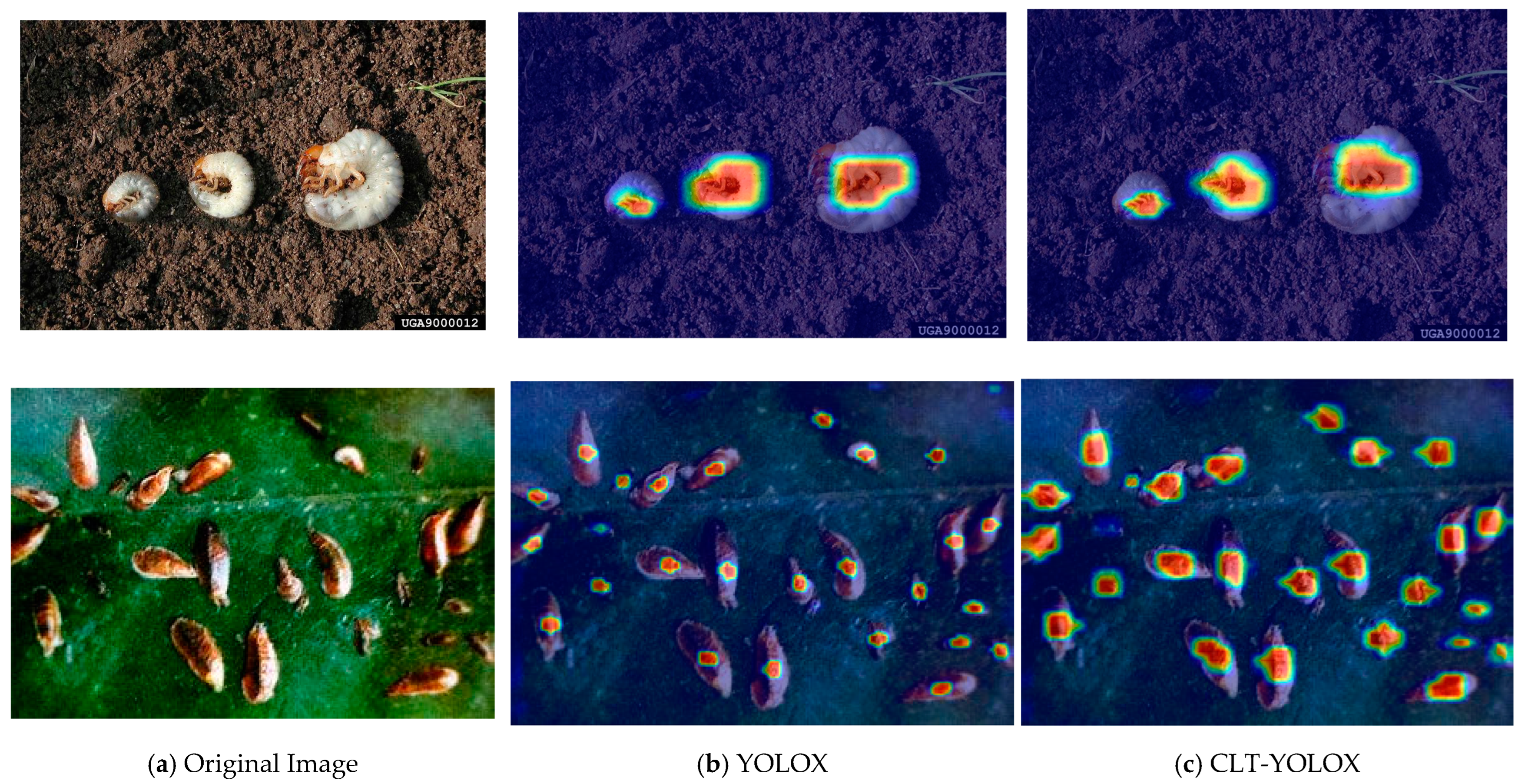
4.4.2. Visualization Comparison of the Thermal Characteristic Maps

We visualize the spatial distribution of regions of interest (ROIs) in the feature maps generated by the small prediction head of CLT-YOLOX, as depicted in Figure 13. In this visualization, each pixel’s color represents the average confidence that the pixel is correctly classified. Higher confidence is represented by a tendency towards red, while lower confidence is indicated by a tendency towards blue.

The second column in Figure 9 shows the results obtained from the original model YOLOX, while the third column shows the results of CLT-YOLOX. It is clear that the improved CLT-YOLOX model exhibits significantly enhanced feature extraction capabilities in detecting pests. The model effectively analyzes more valuable information, resulting in larger regions being highlighted in red, especially for the detection of tiny objects. This demonstrates an improved accuracy in identifying areas of interest associated with pests.

5. Conclusions

In this paper, a novel approach is proposed to address the challenges associated with pest image detection. The combination of Mosaic and Mixup techniques for data preprocessing is introduced to overcome the limitations imposed by small datasets in pest detection. By leveraging these techniques, the model can better handle knowledge limitations and mitigate overfitting issues during the learning process.

To enhance the detection performance specifically in pest identification, several state-of-the-art techniques are incorporated into the model. The C2F module is introduced to capture broader gradient flow information while maintaining a lightweight structure. The CBAM module, known for its simplicity and effectiveness, is utilized to extract attention regions in pest images, aiding in filtering out confusing information and focusing on relevant target objects. Additionally, empirical tricks are employed to further enhance the detection performance of the model.

To expand the scale feature extraction of the network model and improve its expressive ability, the paper introduces shallow information and proposes the CLT module. This module enriches the features of small paths by utilizing information from larger paths, enabling better feature representation and extraction. The CLT module plays a crucial role in improving the model’s expressive ability and contributes to the development of the CLT-YOLOX model.

To validate the effectiveness of each strategy employed in this study, ablation experiments are conducted. These experiments systematically evaluate the impact of different components and techniques on the overall performance of the model. Furthermore, the model’s performance is evaluated on public datasets, which serve as benchmarks for pest image detection. The results demonstrate the efficacy of the proposed approach in accurately detecting pests in various scenarios.

Overall, this paper presents a comprehensive approach that combines various techniques and strategies to address the challenges in pest image detection. The proposed CLT-YOLOX model showcases an improved performance and demonstrates its effectiveness in pest identification tasks.

References

1. Lindeberg, T. Scale Invariant Feature Transform. Scholarpedia 2012, 7, 10491. [Google Scholar] [CrossRef]
2. Ojala, T.; Pietikäinen, M.; Harwood, D. A Comparative Study of Texture Measures with Classification Based on Featured Distributions. Pattern Recognit. 1996, 29, 51–59. [Google Scholar] [CrossRef]
3. Rublee, E.; Rabaud, V.; Konolige, K.; Bradski, G. ORB: An Efficient Alternative to SIFT or SURF. In Proceedings of the 2011 International Conference on Computer Vision, Barcelona, Spain, 6–13 November 2011; IEEE: Piscataway, NJ, USA, 2011; pp. 2564–2571. [Google Scholar]
4. Bay, H.; Tuytelaars, T.; Van Gool, L. Surf: Speeded up Robust Features. Lect. Notes Comput. Sci. 2006, 3951, 404–417. [Google Scholar]
5. Hearst, M.A.; Dumais, S.T.; Osuna, E.; Platt, J.; Scholkopf, B. Support Vector Machines. IEEE Intell. Syst. Appl. 1998, 13, 18–28. [Google Scholar] [CrossRef] [Green Version]
6. Peterson, L.E. K-Nearest Neighbor. Scholarpedia 2009, 4, 1883. [Google Scholar] [CrossRef]
7. Breiman, L. Random Forests. Mach. Learn. 2001, 45, 5–32. [Google Scholar] [CrossRef] [Green Version]
8. Hinton, G.E. Deep Belief Networks. Scholarpedia 2009, 4, 5947. [Google Scholar] [CrossRef]
9. LeCun, Y.; Boser, B.; Denker, J.S.; Henderson, D.; Howard, R.E.; Hubbard, W.; Jackel, L.D. Backpropagation Applied to Handwritten Zip Code Recognition. Neural Comput. 1989, 1, 541–551. [Google Scholar] [CrossRef]
10. Hopfield, J.J. Hopfield Network. Scholarpedia 2007, 2, 1977. [Google Scholar] [CrossRef]
11. Goodfellow, I.; Pouget-Abadie, J.; Mirza, M.; Xu, B.; Warde-Farley, D.; Ozair, S.; Courville, A.; Bengio, Y. Generative Adversarial Networks. Commun. ACM 2020, 63, 139–144. [Google Scholar] [CrossRef]
12. Sabour, S.; Frosst, N.; Hinton, G.E. Dynamic Routing between Capsules. In Proceedings of the Advances in Neural Information Processing Systems 30: Annual Conference on Neural Information Processing Systems 2017, Long Beach, CA, USA, 4–9 December 2017. [Google Scholar]
13. Wu, X. Study on Identification of Pests Based on Machine Vision. Ph.D. Thesis, Zhejiang University, Hangzhou, China, 2016. [Google Scholar]
14. Wang, L.; Sun, J.; Wu, X.; Shen, J.; Lu, B.; Tan, W. Identification of Crop Diseases Using Improved Convolutional Neural Networks. IET Comput. Vis. 2020, 14, 538–545. [Google Scholar] [CrossRef]
15. Huang, M.-L.; Chuang, T.-C.; Liao, Y.-C. Application of Transfer Learning and Image Augmentation Technology for Tomato Pest Identification. Sustain. Comput. Inform. Syst. 2022, 33, 100646. [Google Scholar] [CrossRef]
16. Girshick, R. Fast R-Cnn. In Proceedings of the IEEE International Conference on Computer Vision, Santiago, Chile, 7–13 December 2015; pp. 1440–1448. [Google Scholar]
17. Cui, Y.; Yang, L.; Liu, D. Dynamic Proposals for Efficient Object Detection. arXiv 2022, arXiv:2207.05252. [Google Scholar]
18. Dai, Z.; Cai, B.; Lin, Y.; Chen, J. Up-Detr: Unsupervised Pre-Training for Object Detection with Transformers. In Proceedings of the IEEE/CVF Conference on Computer Vision and Pattern Recognition, Virtual, 19–25 June 2021; pp. 1601–1610. [Google Scholar]
19. Carion, N.; Massa, F.; Synnaeve, G.; Usunier, N.; Kirillov, A.; Zagoruyko, S. End-to-End Object Detection with Transformers. In Proceedings of the Computer Vision–ECCV 2020: 16th European Conference, Glasgow, UK, 23–28 August 2020; Springer: Berlin/Heidelberg, Germany, 2020; pp. 213–229. [Google Scholar]
20. Redmon, J.; Farhadi, A. Yolov3: An Incremental Improvement. arXiv 2018, arXiv:1804.02767. [Google Scholar]
21. Jocher, G.; Stoken, A.; Borovec, J.; NanoCode012; ChristopherSTAN; Liu, C.; Laughing; tkianai; Hogan, A.; lorenzomammana; et al. Ultralytics/Yolov5: V3.1-Bug Fixes and Performance Improvements. 2020. Available online: https://zenodo.org/record/4154370 (accessed on 20 June 2019).
22. Cai, Y.; Luan, T.; Gao, H.; Wang, H.; Chen, L.; Li, Y.; Sotelo, M.A.; Li, Z. YOLOv4-5D: An Effective and Efficient Object Detector for Autonomous Driving. IEEE Trans. Instrum. Meas. 2021, 70, 1–13. [Google Scholar] [CrossRef]
23. Ge, Z.; Liu, S.; Wang, F.; Li, Z.; Sun, J. Yolox: Exceeding Yolo Series in 2021. arXiv 2021, arXiv:2107.08430. [Google Scholar]
24. Bochkovskiy, A.; Wang, C.-Y.; Liao, H.-Y.M. Yolov4: Optimal Speed and Accuracy of Object Detection. arXiv 2020, arXiv:2004.10934. [Google Scholar]
25. Wang, K.; Liew, J.H.; Zou, Y.; Zhou, D.; Feng, J. Panet: Few-Shot Image Semantic Segmentation with Prototype Alignment. In Proceedings of the IEEE/CVF International Conference on Computer Vision, Seoul, Republic of Korea, 27 October–2 November 2019; pp. 9197–9206. [Google Scholar]
26. Tan, M.; Pang, R.; Le, Q.V. Efficientdet: Scalable and Efficient Object Detection. In Proceedings of the IEEE/CVF Conference on Computer Vision and Pattern Recognition, Seattle, WA, USA, 13–19 June 2020; pp. 10781–10790. [Google Scholar]
27. Woo, S.; Park, J.; Lee, J.-Y.; Kweon, I.S. Cbam: Convolutional Block Attention Module. In Proceedings of the European Conference on Computer Vision (ECCV), Munich, Germany, 8–14 September 2018; pp. 3–19. [Google Scholar]
28. Zhang, H.; Cisse, M.; Dauphin, Y.N.; Lopez-Paz, D. Mixup: Beyond Empirical Risk Minimization. arXiv 2017, arXiv:1710.09412. [Google Scholar]
29. Yun, S.; Han, D.; Oh, S.J.; Chun, S.; Choe, J.; Yoo, Y. Cutmix: Regularization Strategy to Train Strong Classifiers with Localizable Features. In Proceedings of the IEEE/CVF International Conference on Computer Vision, Seoul, Republic of Korea, 27 October–2 November 2019; pp. 6023–6032. [Google Scholar]
30. Hassan, S.N.; Rahman, N.S.; Win, Z. Automatic Classification of Insects Using Color-Based and Shape-Based Descriptors. Int. J. Appl. Control Electr. Electron. Eng. 2014, 2, 23–35. [Google Scholar]
31. Zheng, C.-H.; Pei, W.-J.; Yan, Q.; Chong, Y.-W. Pedestrian Detection Based on Gradient and Texture Feature Integration. Neurocomputing 2017, 228, 71–78. [Google Scholar] [CrossRef]
32. Shen, Y.; Zhou, H.; Li, J.; Jian, F.; Jayas, D.S. Detection of Stored-Grain Insects Using Deep Learning. Comput. Electron. Agric. 2018, 145, 319–325. [Google Scholar] [CrossRef]
33. Rani, R.U.; Amsini, P. Pest Identification in Leaf Images Using SVM Classifier. Int. J. Comput. Intell. Inform. 2016, 6, 248–260. [Google Scholar]
34. Chen, Q.; Wang, Y.; Yang, T.; Zhang, X.; Cheng, J.; Sun, J. You Only Look One-Level Feature. In Proceedings of the IEEE/CVF Conference on Computer Vision and Pattern Recognition, Virtual, 19–25 June 2021; pp. 13039–13048. [Google Scholar]
35. He, Y.; Zhou, Z.; Tian, L.; Liu, Y.; Luo, X. Brown Rice Planthopper (Nilaparvata Lugens Stal) Detection Based on Deep Learning. Precis. Agric. 2020, 21, 1385–1402. [Google Scholar] [CrossRef]
36. Duan, K.; Bai, S.; Xie, L.; Qi, H.; Huang, Q.; Tian, Q. Centernet: Keypoint Triplets for Object Detection. In Proceedings of the IEEE/CVF International Conference on Computer Vision, Seoul, Republic of Korea, 27 October–2 November 2019; pp. 6569–6578. [Google Scholar]
37. Yang, Z.; Liu, S.; Hu, H.; Wang, L.; Lin, S. Reppoints: Point Set Representation for Object Detection. In Proceedings of the IEEE/CVF International Conference on Computer Vision, Seoul, Republic of Korea, 27 October–2 November 2019; pp. 9657–9666. [Google Scholar]
38. Huang, J.; Huang, Y.; Huang, H.; Zhu, W.; Zhang, J.; Zhou, X. An Improved YOLOX Algorithm for Forest Insect Pest Detection. Comput. Intell. Neurosci. 2022, 2022, 5787554. [Google Scholar] [CrossRef]
39. Zhao, Q.; Liu, B.; Lyu, S.; Wang, C.; Zhang, H. TPH-YOLOv5++: Boosting Object Detection on Drone-Captured Scenarios with Cross-Layer Asymmetric Transformer. Remote Sens. 2023, 15, 1687. [Google Scholar] [CrossRef]
40. Zhang, X.; Zeng, H.; Guo, S.; Zhang, L. Efficient Long-Range Attention Network for Image Super-Resolution. In Proceedings of the Computer Vision–ECCV 2022: 17th European Conference, Tel Aviv, Israel, 23–27 October 2022; Springer: Berlin/Heidelberg, Germany, 2022; pp. 649–667. [Google Scholar]
41. Wang, C.-Y.; Liao, H.-Y.M.; Wu, Y.-H.; Chen, P.-Y.; Hsieh, J.-W.; Yeh, I.-H. CSPNet: A New Backbone That Can Enhance Learning Capability of CNN. In Proceedings of the IEEE/CVF Conference on Computer Vision and Pattern Recognition Workshops, Seattle, WA, USA, 14–19 June 2020; pp. 390–391. [Google Scholar]
42. Li, Y.; Yao, T.; Pan, Y.; Mei, T. Contextual Transformer Networks for Visual Recognition. IEEE Trans. Pattern Anal. Mach. Intell. 2022, 45, 1489–1500. [Google Scholar] [CrossRef]
Figure 1. The enhanced CLT-YOLOX model introduces a Cross-Layer Transformer module that integrates two layers of features to generate the output of the target detection head, distinguishing it from the original YOLOX.
Agronomy 13 02091 g001
Figure 2. CLT-YOLOX replaces the C3 module in the original neck structure with the C2F module, cancels the convolution operation before the upsampling stage, adds CBAM attention, and proposes a CLT Cross-Layer Transformer module to enrich the small path feature. CLT takes f 1 and f 2 as input and output f 2 , and when the calculated result is connected to f 2 , it performs another convolution and enters the prediction stage.
Agronomy 13 02091 g002
Figure 3. Mosaic and Mixup data enhancement visualization.
Agronomy 13 02091 g003
Figure 4. Focus module and SPP module structure diagram: (a) is the focus structure schematic diagram; (b) is the schematic diagram of the SPP module.
Agronomy 13 02091 g004
Figure 5. C2F module and C3 module structure diagram: the left picture is the C2F module, and the right picture is the C3 module. It can be seen that the left picture achieves a richer information flow by parallelizing more branches.
Agronomy 13 02091 g005
Figure 6. CBAM module structure diagram.
Agronomy 13 02091 g006
Figure 7. The figure shows the flow of the CLT module and the number of characteristic channels in each step.
Agronomy 13 02091 g007
Figure 8. The architecture of our CLT module, as shown in the figure, depicts the generation of Q and K from f 1 , while V is generated from f 2 . This CLT design enables the effective extraction of asymmetric information between the two paths and enriches the feature.
Agronomy 13 02091 g008
Figure 9. IP102 dataset distribution.
Agronomy 13 02091 g009
Figure 10. (a) represents the decline curve of the model training loss; (b) represents the decline curve of the model verification loss; (c) represents the change curve of the mAP of the model during training. The gray line represents the original model YOLOX, the blue line represents the YOLOX that uses our enhanced strategy and frozen training, and the red line represents our final improved model, CLT-YOLOX.
Agronomy 13 02091 g010
Figure 11. The blue box represents the real label of the image, and the green box represents the prediction box of the model.
Agronomy 13 02091 g011
Figure 12. The figure displays instances of matching failures. In the first row, the similarity in shape and appearance between the objects can be attributed as the reason for the failure. In the second row, the images correspond to different growth stages of the same pest species, which causes the mismatch in detection results. The blue box represents the real label of the image, and the green box represents the prediction box of the model, and the red box indicates that the detection result fails to match the real result.
Agronomy 13 02091 g012
Figure 13. The above figure shows the experimental specific heat map Higher confidence is represented by a tendency towards red, while lower confidence is in-dicated by a tendency towards blue.
Agronomy 13 02091 g013