Article

Integrating Spectral, Textural, and Morphological Data for Potato LAI Estimation from UAV Images

1
School of Surveying and Land Information Engineering, Henan Polytechnic University, Jiaozuo 454000, China
2
Information Technology Research Center, Beijing Academy of Agriculture and Forestry Sciences, Beijing 100097, China
3
National Engineering and Technology Center for Information Agriculture, Nanjing Agricultural University, Nanjing 210095, China
*
Authors to whom correspondence should be addressed.
Agronomy 2023, 13(12), 3070; https://doi.org/10.3390/agronomy13123070
Submission received: 28 November 2023 / Revised: 7 December 2023 / Accepted: 14 December 2023 / Published: 15 December 2023
(This article belongs to the Special Issue Application of Remote Sensing and GIS Technology in Agriculture)

Abstract

:
The Leaf Area Index (LAI) is a crucial indicator of crop photosynthetic potential, which is of great significance in farmland monitoring and precision management. This study aimed to predict potato plant LAI for potato plant growth monitoring, integrating spectral, textural, and morphological data through UAV images and machine learning. A new texture index named VITs was established by fusing multi-channel information. Vegetation growth features (Vis and plant height Hdsm) and texture features (TIs and VITs) were obtained from drone digital images. Various feature combinations (VIs, VIs + TIs, VIs + VITs, VIs + VITs + Hdsm) in three growth stages were adopted to monitor potato plant LAI using Partial Least Squares Regression (PLSR), Support Vector Regression (SVR), random forest (RF), and eXtreme gradient boosting (XGBoost), so as to find the best feature combinations and machine learning method. The performance of the newly built VITs was tested. Compared with traditional TIs, the estimation accuracy was obviously improved for all the growth stages and methods, especially in the tuber-growth stage using the RF method with 13.6% of R2 increase. The performance of Hdsm was verified by including it either as one input feature or not. Results showed that Hdsm could raise LAI estimation accuracy in every growth stage, whichever method is used. The most significant improvement appeared in the tuber-formation stage using SVR, with an 11.3% increase of R2. Considering both the feature combinations and the monitoring methods, the combination of VIs + VITs + Hdsm achieved the best results for all the growth stages and simulation methods. The best fitting of LAI in tuber-formation, tuber-growth, and starch-accumulation stages had an R2 of 0.92, 0.83, and 0.93, respectively, using the XGBoost method. This study showed that the combination of different features enhanced the simulation of LAI for multiple growth stages of potato plants by improving the monitoring accuracy. The method presented in this study can provide important references for potato plant growth monitoring.

1. Introduction

Potato is the fourth largest food crop in the world [1], and the healthy development of the potato industry is of great significance to global food security. China’s potato cultivation area ranks first globally, but the unit yield is lower than the world average [2]. In recent years, with the intensification of global environmental change and the increasing concern for ecosystem function and health, accurate monitoring and assessment of surface vegetation has become an important research area [3]. As one of the critical indicators of vegetation growth, the Leaf Area Index (LAI) has essential applications in vegetation ecology, agricultural production, and ecosystem management [4]. LAI reflects the vegetation biomass, the intensity of photosynthesis, and the exchange of energy and matter [5]. Accurately obtaining and monitoring LAI is significant for understanding vegetation’s growth status and ecosystems’ structure and function [6]. Traditional LAI measurement methods are mostly field sampling surveys, which can damage the plants in the acquisition process and thus cause crop-yield reduction [7]. The optical LAI-based measurement instruments require the experience of testers to choose the appropriate time and operation method, which encounters the problems of high time and space costs and it is difficult to monitor continuously and on a large scale. With the development of remote-sensing technology, satellites, aerial aircrafts, and Unmanned Aerial Vehicles (UAVs) have become effective methods for large-scale crop-growth monitoring [8]. Croft [9] developed a chlorophyll-monitoring model for wheat and maize using the Landsat-8 multispectral satellite. Moharana [10] constructed a model for measuring nitrogen and chlorophyll content of rice using EO-1 Hyperion hyperspectral data and ground-based spectroradiometer measurements. The look-up table (LUT) of the PROSAIL model combined with the hyperspectral UAV was also applied to estimate the inversion potato LAI [11]. Clevers [12] used Sentinel-2 satellite images to estimate the LAI, leaf chlorophyll content (LCC), and canopy chlorophyll content (CCC) of potatoes through vegetation indices. Although satellite data can assess various nutrient indicators of crops on a large scale, its application in precision agriculture is limited by its long revisit period, atmospheric cloud cover, and low spatial resolution [13]. UAV is widely used due to its low price, easy maneuverability, and simple data processing [14,15,16].
The vegetation indices can quickly provide information about vegetation growth status, dynamic changes, vegetation classification, cover estimation, etc., and are widely used in crop-nutrition monitoring. Du [17] used drones to collect maize canopy spectral information, construct 14 vegetation indices, and use linear regression and neural network models to establish LAI estimation models. Hasan [18] used UAV red, green, and blue (RGB) images to estimate the LAI of winter wheat at the jointing stage of Xinjiang. He constructed a Partial Least Squares Regression (PLSR) model based on the Visible Atmospheric Resistant Index (VARI), Red–Green–Blue Vegetation Index (RGBVI), Blue (B), and Green Leaf Algorithm (GLA). Yamaguchi [19] combined deep learning (DL) with UAV RGB and multispectral images to construct the best model of rice LAI based on DL. However, due to the vegetation canopy’s spectral saturation and canopy-structure complexity, the results were inaccurate when estimating only using the vegetation index (VI) [20].
In response to the phenomenon of spectral saturation observed in canopy spectra, researchers have been systematically exploring various methodologies to augment the accuracy of crop-nutrition monitoring. This endeavor primarily focuses on diminishing the impact of spectral saturation on the precision of predictive results. UAV multispectral imagery combines these two kinds of Square Multilayer Perceptron (MLP), and Least Squares Support Vector Machine (LS-SVM). Moreover, it was compared with linear regression to estimate potato LAI when LAI was at its maximum in the field [21]. Fan [22] constructed six spectral transformations, 12 arbitrary band combinations, and the best estimation model for potato plant nitrogen content (PNC) using the three-band spectral index. Some studies have introduced new image features to reduce the effect of spectral saturation. Yue [15] solved the problem of underestimation of winter wheat AGB using ultra-high-ground-resolution image texture, VI, and their combinations. Liu [23] estimated the nitrogen nutrition index (NNI) based on drone VI and texture features and found that the average VI of all pixels in the region of interest (ROI) was better than the average of vegetation pixels within the ROI. Some studies have introduced morphological parameters to address crop-canopy spectral saturation. Qiao [24] used a multispectral sensor carried using UAV to collect remote-sensing images of the maize canopy at six growth stages. The LAI estimation model was constructed based on the fusion of morphological parameters and vegetation index features. Lu [25] combined UAV spectral and structural information, introduced a canopy-height model, and alleviated LAI overestimation using canopy coverage as a correction parameter. The results showed that the wheat LAI estimation model using fusion parameters improved the accuracy of (RGB) images by 43.6%. Yan [26] used UAV multispectral cameras and Light Detection and Ranging (LiDAR) sensors to obtain multi-source data of cotton fields and constructed a cotton LAI estimation model based on fused data. Zhang [27] built a kiwifruit LAI inversion model by comparing stepwise regression (SWR) and random forest regression (RFR) by combining vegetation index and texture characteristics. Some studies combined vegetation index with texture features and morphological parameters. Zhang [28] combined the color index, vegetation index, and canopy height extracted using UAV RGB, and the results showed that the accuracy of the LAI model in the four growth stages of wheat was improved after adding plant-height information. Wu [29] acquired high-resolution drone images, extracted the wheat canopy’s spectra structural and thermal features, and removed the LAI estimation using random forest and Support Vector Machine Regression. Liu [30] solved the problem of underestimating the high AGB values of potato samples by using only RGB-VI modeling, combined with Gray-level covariance matrix (GLCM) based textures acquired using UAV digital images, and heigh of digital surface model (Hdsm) and RGB-VIs can improve the accuracy of potato AGB estimation at high coverage. Yu [31] combined UAV RGB imagery, LiDAR, and hyperspectral imagery to construct a potato LAI model with multi-feature fusion. They found that the hyperspectral vegetation index was the most critical feature of the model.
The above studies show that combining vegetation index, texture, and morphological parameter information can further improve the estimation accuracy of LAI. However, there are some limitations: (1) a single texture index makes it difficult to reflect the complex changes in the crop-canopy structure, resulting in the addition of texture information to improve the accuracy of the model which is not apparent; (2) it is challenging to use only the canopy spectral or structural information to provide the information on the changes in LAI of different dimensions which leads to poor monitoring accuracy. In this study, a new feature vegetation index improves texture (VIT) and was obtained by calculating the texture information of different spectral channels and indexing it to explore the effect of different combinations of textures on crop LAI monitoring more deeply. Moreover, plant height was added to the model as a feature—in the vertical direction of the crop—to explore the effect of the fusion of multiple types of features to estimate LAI. The machine learning method SVR-RFE was used to rank the VIs, TIs, and VITs. The top three ranked features were selected. Plant height was added to the model as a feature in both vertical directions. Four models, Partial Least Squares Regression (PLSR) [32], Support Vector Regression (SVR) [33], random forest (RF) [30], and eXtreme gradient boosting (XGBoost) [34], were used to model the LAI estimation of potato plants over multiple growth stages.

2. Materials and Methods

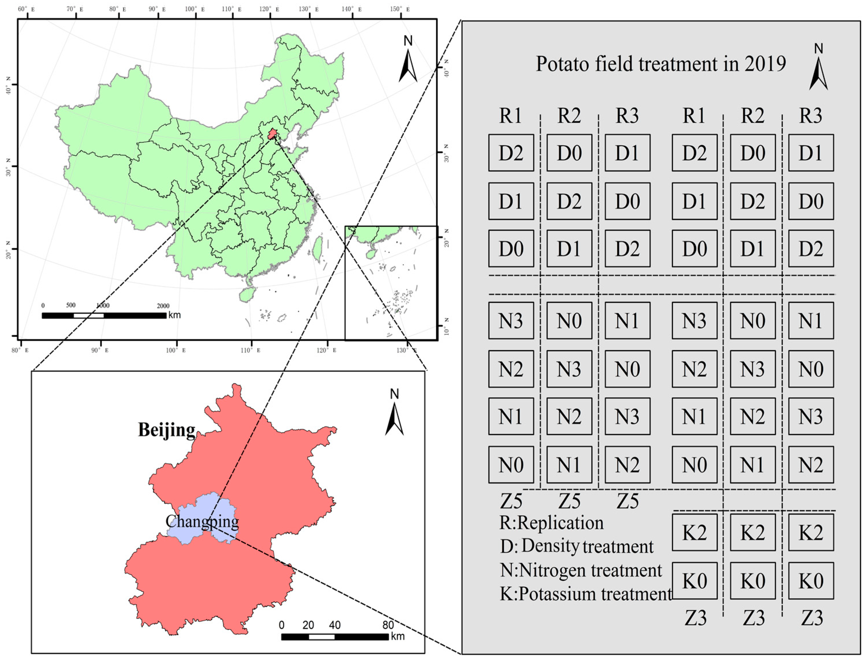
2.1. Study Area and Experimental Design

This study was conducted in 2019 at the National Precision Agriculture Research Demonstration Base in Xiaotangshan Town, Changping District, Beijing, China. The experimental area was in the eastern part of Xiaotangshan Town (40°10′34″ N, 116°26′39″ E). The practical site has a warm-temperate continental semi-humid and semi-arid monsoon climate, characterized by four distinct seasons, rain and heat in the same season, with a multi-year average temperature of 11.8 °C, an average elevation of 34 m, an average of 2816 h of sunshine per year, an average of 584 mm of precipitation per year, and an average of 203 days of a frost-free period per year. The experimental area adopts a plot-gradient fertilization design, with 48 plots (5 m × 6.5 m), and selects early-maturing potato varieties Zhongshu5 (Z5) and Zhongshu3 (Z3) as experimental varieties. Three density gradients (d1: 60,000 plants/hm2, d1: 72,000 plants/hm2, d2: 84,000 plants/hm2) were set in zone D; nitrogen fertilizer was N2, and potassium fertilizer was K1 (495 kg/hm2). Four nitrogen gradients (N0: 0 kg/hm2, N1: 112.5 kg/hm2, N2: 225 kg/hm2, N3: 337.5 kg/hm2) pure N were set in zone N, density is D1, K fertilizer was K1. For two potassium gradient experiments (K0: 0 kg/hm2, K2: 990 kg/hm2), K2O was set in zone K, density was D1, N fertilizer was N2. The phosphorus fertilizer for all plots was 90 kg/hm2. The NPK gradient was provided using urea, superphosphate, and potassium sulfate. Eleven ground control points were uniformly set in the experimental plots to ensure image-stitching accuracy, and a high-precision differential positioning system (GPS) was used for millimeter-level positioning. The study area and experimental plot setting are shown in Figure 1.

2.2. Data Collection

2.2.1. UAV Image Acquisition and Processing

This study utilized a DJI phantom4 digital camera (SZ DJI Technology Co., Ltd., Shenzhen, China) as a remote-sensing platform to acquire UAV spectral images; the camera was equipped with a 1-inch CMOS sensor with 20 million effective pixels, a lens field of view of 84°, a focal length of 8.8 mm, and a maximum photographic resolution of 4000 × 3000. The specific parameters of the sensor are shown in Table 1. Digital images of potato tuber formation, growth, and starch accumulation were obtained. The flight altitude was 20 m, data collection was from 10 a.m. to 2 p.m., the overlap rate between routes was 85%, and data acquisition was carried out under clear, windless, and cloudless weather conditions. The images were checked for any deficiencies after each flight. The orthophoto (DOM) and elevation image (DSM) were obtained using PhotoScan software (Agisoft LL., St. Petersburg, Russia) for correction and image stitching. The processing steps are as follows: (1) POS import: import the images in the airstrip and the corresponding POS points into the PhotoScan software to restore the geographic position of the route photos. (2) Image alignment: add the ground control points to the software to optimize the image alignment accuracy and generate the 3D point cloud of the flight area using its three-coordinate information. (3) Product generation: generate a spatial grid based on the 3D point cloud and create texture information to generate DOM and DEM. (4) Radiometrically correct the orthophoto using ENVI5.3 (Exelis Visual Information Solution., Boulder, CO, USA) to convert the numbers (DNs) to reflectance.

2.2.2. Ground Data Acquisition and Processing

Ground data acquisition was synchronized with UAV data collection. We manually acquired potato plants destructively on May 28 (tuber-formation stage, S1), June 10 (tuber-growth stage, S2), and June 20 (starch-accumulation stage, S3). We selected three typical potato plants from each plot and calculated the area they occupied (A) through planting density. Then, we sampled and separated their stems and leaflets. Twenty pieces of representative leaflets were selected, from which a circular area with a diameter of 0.8 cm was perforated and collected from every selected leaflet. The total area S of these collected parts was recorded, as well as their dry weight W1 after drying in the oven. The remaining leaflets were dried and weighed too (W2). As shown in Equation (1), LAI (m2/m2) was calculated using a specific leaf weight method. The plant height of each plot was measured using the average of five seedlings selected from the plot.
L A I = W 1 + W 2 W 1 × A × 10000 × S
A = 10000 D × 3

2.3. Parameter Extraction

2.3.1. Selection of Vegetation Indices

The vegetation index combines different bands of digital images in a certain way to reduce or eliminate the influence of background information on crop-canopy spectra. In this paper, 28 spectral bands and vegetation indices were selected to invert potato LAI according to previous research results, and the canopy reflectance was averaged for each round in interest within the range of 5 m × 6.5 m. The specific names and calculation formulas are shown in Table 2.

2.3.2. Acquisition of Texture Features

Gray-level covariance matrix (GLCM) extraction was performed on digital orthophotos with a window of 3 × 3 pixels using ENVI v.5.3 software, and eight types of gray-level covariance matrix-based texture eigenvalues were calculated for each plot: mean (Mean), homogeneity (Hom), entropy (Entropy, Ent), dissimilarity (Dis), second moment (Sec), correlation (Cor), variance (Var), contrast (Con). To fully use the vegetation information contained in different channels of texture index, the three channels (RGB) of 8 texture indexes were calculated according to 14 vegetation index formulas (Table 3), and 112 improved-texture indexes were obtained. See Table 4.

2.3.3. Potato-Plant-Height Extraction at Different Growth Stages

Potato-plant-height extraction took place using UAV images and GCPs of the test area. DSMs for each period of the trial were generated using PhotoScan, and by calculating the difference between the DSMs of the different periods of the potato and bare soil, potato plant height Hdsm could be obtained for each growth stage.

2.4. Modeling and Assessment

2.4.1. Feature-Screening Methods

The Recursive Feature Elimination (RFE) method performs a widely used wrapper feature selection model using iteration, which has performed well in previous studies [44]. Our study adopts the SVR feature screening method for feature selection [45]. SVR is a machine learning method commonly used for regression prediction, which is based on the theory of Support Vector Machines (SVM) and has been improved to deal with continuous variables. SVR is well suited for feature screening as it can capture complex nonlinear relationships. When performing feature screening, we first use all the features for training the SVR model and record the importance of each feature, which is usually obtained by looking at the weights of each feature in the SVR model. Then, we rank all features according to their importance. In general, features with higher importance significantly impact the model’s prediction results, so we select features with higher importance for subsequent model training. We then use a looping process to remove the features with the lowest importance one by one, and after each removal of a feature, we retrain the SVR model and test its performance. If the model’s performance does not degrade significantly after removing a feature, then we permanently remove that feature. We repeat this process until removing any features significantly degrades the model performance. With this approach, we can filter out the features that have the most significant impact on the model’s prediction results while removing the features that have less impact on the results, thus simplifying the model and improving its prediction accuracy.

2.4.2. Modeling Methodology

Four methods, PLSR, RF, SVR, and XGBoost, were used for potato LAI estimation.
(1)
PLSR is a statistical method that attempts to find a linear regression model between the set of observed variables (X) and the set of predictor variables (Y) that optimizes prediction by minimizing the sum of the squares of prediction errors. In some complex problems, the PLSR model has advantages over the multiple linear regression model.
(2)
The RF model is a prediction model based on decision trees using the Ensemble Learning strategy. It combines the prediction results of multiple decision trees to improve the prediction accuracy and robustness of the overall model. Its characteristics give it excellent performance in solving various prediction problems, including classification and regression problems.
(3)
SVR is an application of SVM to regression problems. SVR provides an effective way to keep the prediction error for the training samples within a given threshold while keeping the model complexity as small as possible. SVR can handle high-dimensional data and has good performance for nonlinear problems. Data are robust to nonlinear problems and have good generalization capabilities.
(4)
XGBoost is an efficient machine learning algorithm based on gradient-boosting decision trees, which has shown excellent performance in many machine learning tasks, including classification, regression, and sorting problems. It employs a forward stepwise addition strategy that corrects the prediction errors of all previous trees by continuously adding new trees.

2.4.3. Model Validation and Evaluation

This study used Leave-One-Out Cross Validation (LOOCV) as the dataset segmentation method. LOOCV is a commonly used model-validation method designed to assess the generalization performance of a model. LOOCV is mainly applied to small-sample datasets because, in this case, other cross-validation methods (e.g., k-fold cross-validation) may result in a split between the training and validation sets that are too extreme. The 48 sets of data for each growth stage and the actual field measurement dataset were divided into 41 training sets and one test set, where each sample was predicted only once. The average value was finally selected as the final performance of the model. The Coefficient of Determination (R2), Root Mean Squared Error (RMSE), and Mean Absolute Error (MAE) were also used as the model accuracy-evaluation indices.

3. Results

3.1. LAI and Plant Height of Potatoes at Different Growth Stages

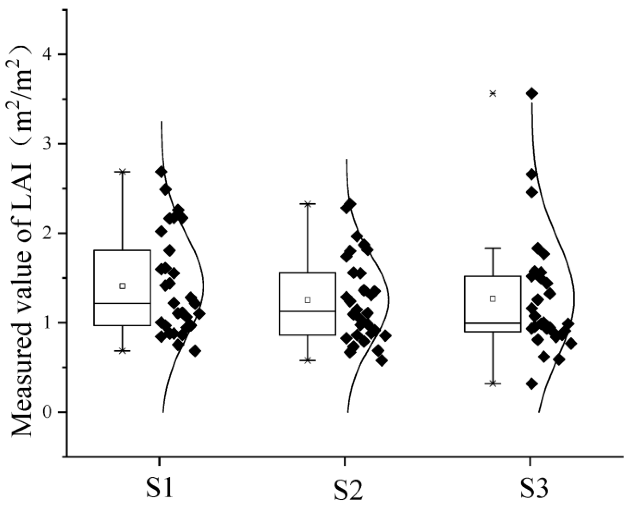
3.1.1. Distribution of LAI in Potatoes at Different Growth Stages

Three field experiments were conducted to determine LAI for 48 Test areas. A total of 144 LAI samples were obtained during the three growing periods, as shown in Figure 2. The potato LAI box line plot reflects the stage changes of LAI in the potato canopy. LAI values decreased from tuber formation to tuber growth, but the change was flat, and LAI remained stable from tuber growth to starch accumulation. The LAI ranges from 0.46 to 2.69 m2/m2 in the tuber-formation stage, with an average LAI of 1.38 m2/m2; the LAI ranged from 0.35 to 2.49 m2/m2 in the tuber-growth stage, with an average LAI of 1.26 m2/m2; the LAI ranged from 0.29 to 3.56 m2/m2 in the starch-accumulation stage, with an average leaf LAI 1.28 m2/m2.

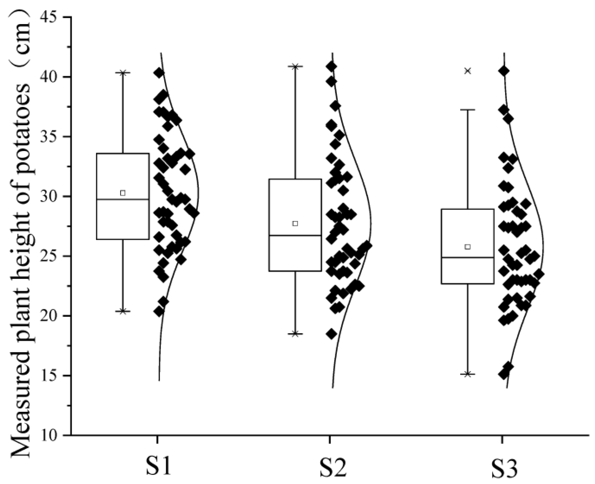
3.1.2. Distribution of Plant Height of Potato Plants at Different Growth Stages

Figure 3 is a box plot of plant-height distribution of potato plants in three growth periods. From the figure, the plant height of potatoes in three growth periods gradually showed a decreasing trend because of the rapid growth of plants in the tuber-growth period in the early stage of potato plants development for the transfer of nutrients; photosynthesis is wholly used for plant development, a large amount of organic matter in the tuber-growth period is transferred to the underground tuber part through the plant, making the plant height of potato plants decrease. During the starch-accumulation period, the organic matter of the aboveground plant part is also transferred to the tuber, making the aboveground plants’ further senescence and the plant height to decrease. During the starch-accumulation period, organic matter from the aboveground plant parts is also transferred to the tubers, causing further senescence of the aboveground plants and a further reduction in plant height. The tuber-formation-period plant height (H) ranged from 20.4 to 40.4 cm, with an average H of 30.3 cm; the tuber-growth period H ranged from 18.5 to 40.9 cm, with an average H of 27.7 cm; and the starch-accumulation period H ranged from 15.1 to 40.5 cm, with an average H of 25.8 cm.

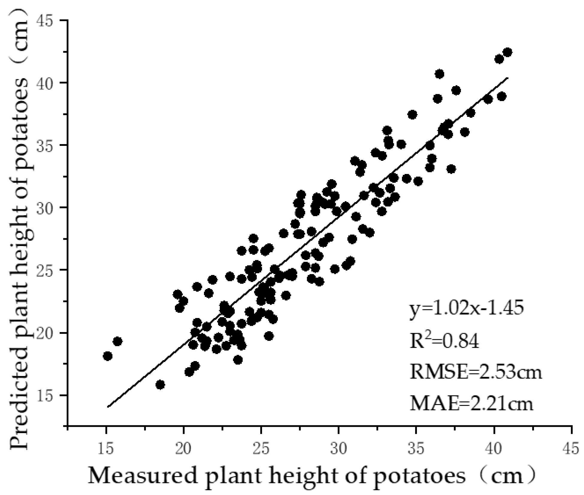
3.2. Validation of Potato-Plant-Height Extraction

In order to verify the accuracy of the potato-plant-height extracted based on DSM, the plant height Hdsm of the three growth stages was compared with the measured plant height H to conduct the validation analysis. The results are shown in Figure 4. The comparison of the potato plant Hdsm of multiple growth stages was extracted based on the DSM data with the measured plant height H and it showed that the R2 was 0.84, the MAE was 2.21 cm, and the RMSE was 2.53 cm.

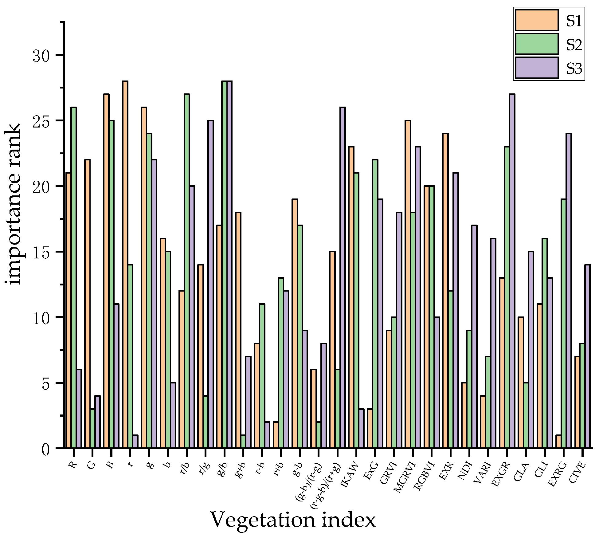
3.3. Materiality Analysis

Figure 5 displays the SVR-RFE method’s ranking of 28 VIs, derived from digital images capturing tuber-formation, -growth, and starch-accumulation stages. In-band three: The ranking results of the 28 spectral vegetation indices, 24 texture parameters, and 112 construction indices (VITs), each assessed separately, are presented in Table 4. According to Figure 5, the ‘g’ and ‘EXG’ indices received high rankings for band importance across all three growth stages.
From Figure 6, B-Var-1, G-Ent-4, G-Ent-2, G-Mean-1, B-Sec-2, G-Ent-3, B-Mean-1, G-Ent-1, B-Mean-3, G-Mean-2 are more advanced in the indexed importance ranking of texture.
Table 4 shows the ranking importance of VITs. TIs changed with MGRVI, VARI, GLA, and GLI features which occupy 87% of the top-ten importance rankings. For clarity, we number texture calculations in the table. m-1 means feature mean with texture information for the TIKAW calculation.

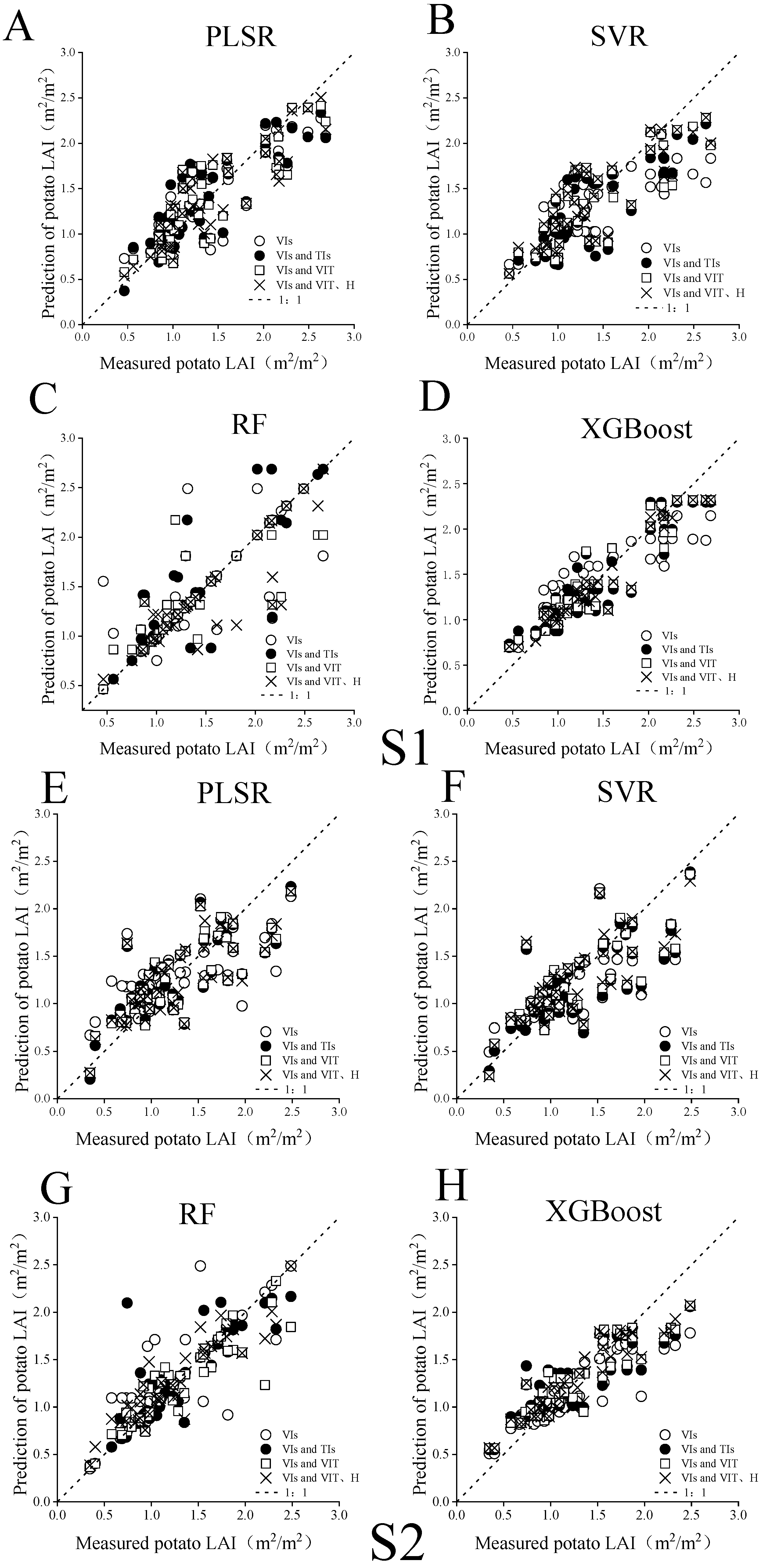
3.4. Model Feature Selection and Modeling

To construct the optimal LAI inversion model, the VIs, TIs, and VITs variables, which rank as the top three in terms of importance, are selected as modeling features, and the leave-one-out validation method is adopted for modeling and finding the best LAI inversion model. In this study, we used the linear modeling approach PLSR, machine learning methods SVR and RF, and XGBoost to model the fusion of VIs, VIs and Tis; VIs and VITs; VIs and VITs; and Hdsm, respectively. We predicted LAI during the tuber-formation period, the tuber-growth period, and the starch-accumulation period of potatoes’ LAI prediction. The study evaluated the models’ performance and accuracy using R2, MAE, and RMSE. The results are shown in Table 5.

4. Discussion

4.1. Spectral and Textural Materiality Ranking with LAI Using SVR-RFE

Traditional feature-selection methodologies, such as the Pearson Correlation Coefficient, are frequently employed in remote-sensing data analysis. However, the Pearson method is limited to delineating superficial linear relationships between features and target values. This study introduces the SVR-RFE approach as a robust alternative. SVR-RFE can address non-linear relationships between features and target variables, and it offers a global observation of all features, thereby circumventing the oversight of complex interplays among multiple characteristics. Furthermore, the RFE component of this method enhances the interpretability of variable selection. Overall, the SVR-RFE feature selection methodology stands out for its flexibility and broad applicability, particularly when features exhibit non-linear relationships with targets or when the data is embedded with noise [46].
After the VIs of the three growth stages were sorted using SVR-RFE, the top 10 in terms of importance in the tuber-formation and tuber-growth stages were g, EXG, B, IKAW, R, RGBVI, and the top 10 in terms of volume in the tuber-growth and starch-accumulation stages were g, EXG, g/b, r/b, EXGR, and EXRG, and the top 10 in terms of importance in the tuber-formation and starch-accumulation stages were g, EXG, g/b, r/b, EXGR, and EXRG, and the top 10 in terms of importance in the tuber-formation and starch-accumulation stages were g, EXG, g/b, r/b, EXGR, and EXRG. In all three growth stages, the top 10 in importance are g and EXG bands, and in RGB images, g represents the normalized green band. Plant chlorophyll has a high reflectance of green light, which makes healthy plants appear visually green. This phenomenon stems from the need for plant photosynthesis. Plant chlorophyll absorbs blue and red light for photosynthesis but less green light. As a result, green light is reflected to our eyes or image sensors, making plants appear green to the human eye or camera. EXG is often used to monitor the growth and greenness of vegetation [47]. In the case of vigorous vegetation growth and dense foliage, LAI tends to be higher, and EXG may also be higher because more foliage causes more green light to be reflected. The EXG index has many applications in remote sensing, environmental science, agriculture, and other fields [36]. It can be used to monitor the growth status of vegetation to optimize irrigation and fertilization strategies.
From the Vis’ features that ranked in the top 10 in importance in the two growth stages, it can be seen that six features classified in the top 10 in volume in both adjacent growth stages, while there were only three in the tuber-formation and starch-accumulation periods, which indicated that there was not much spectral change of the vegetation canopy in the adjacent growth stages and that in the starch-accumulation period, the canopy spectra and the tuber-formation period underwent a more pronounced change due to the beginning of the potato nutrient transfer from the stem and leaflets to the fruits. While texture index and VIs were different, the order of texture importance realized a significant difference in the tuber-growth and starch-accumulation periods, and this change was due to the difference in morphological changes of the plants in different growth stages.
After SVR-RFE sorting, VITs changed with TMGRVI, TVARI, TGLA, and TGLI make up 87% of the top 10 in the importance ranking. The equation of VITs shows that the other three variations, except TMGRVI, contain three channels of this texture. This indicates that combining different band channels can make the texture information more useful in crop-LAI monitoring.

4.2. Effects of Texture and Plant Height on the Accuracy of Estimating Potato LAI at Different Growth Stages

Texture and height information has been widely used for parameter estimation of various crops such as winter wheat [48], maize [49], rice [50], etc. These studies sought suitable vegetation indices and texture as feature input models but did not consider the fusion of texture data from different channels and vertically oriented crop information. In this study, the texture indices extracted from the three tracks were transformed according to 14 commonly used vegetation index formulas to obtain new VIT features. The texture that has been changed with MGRVI, VARI, GLA, and GLI in the newly acquired features occupies 87% in the top 10 in the importance rankings, which suggests that the texture information between the different channels is transformed by specific indices to better respond to the potato LAI information. From the above four texture-calculation methods, all four are the ratio form of the vegetation index. The ratio vegetation index is also the most commonly used for assessing the growth status of vegetation texture information after the ratio calculation [45].
In this study, the accuracy of different data fusion for potato predicted LAI was compared, and the accuracy of the model increased after the fusion of characteristics at the three growth stages. In the tuber-formation stage, the R2 of the PLSR models VIs, VIs + TIs, VIs + VITs, VIs + VITs + Hdsm increased by 6.0%, 10.4%, and 13.4%. The R2 of the SVR model increased by 22.6%, 24.5%, and 35.8%. The R2 of the RF model increased by 14.8%, 18.0%, and 24.6%. The R2 of XGBoost increased by 22.5%, 22.5%, and 29.6%. From the results, feature fusion improves the accuracy of the LAI prediction model. This is consistent with previous studies [50,51]. In the tuber-growth stage, the R2 of the PLSR models VIs, VIs + TIs, VIs + VITs, VIs + VITs + Hdsm were increased by 50%, 50%, and 52.5%. The R2 of the SVR model increased by 3.7%, 7.4%, and 11.1%. The R2 of the RF model increased by 7.6%, 21.2%, and 27.3%. The R2 of XGBoost increased by 2.9%, 13%, and 20.3%. In the starch accumulation, the R2 of PLSR model VIs, VIs + TIs, VIs + VITs, VIs + VITs + HDSM increased by 60.4%, 72.1%, and 74.4%. The R2 of the SVR model increased by 15.8%, 22.8%, and 24.6%. The R2 of the RF model increased by 30.2%, 34.9%, and 39.7%; The R2 of XGBoost increased by 13.2%, 21.1%, and 22.4%. When the TEX improves potato LAI greatly, the accuracy of VITs is lower, while when the TEX improves, the accuracy is smaller, and VITs’ increase is higher. The effect of plant-height characteristics in potato LAI estimation was not obvious in the PLSR model. However, the effect was better in the tuber-formation and growth stages but worse in the starch-accumulation stages, and because potato crops’ growth habits are related, potato stolon’s plant height decreases. At the same time, the LAI gradually increases during the starch-accumulation period, so Hdsm is limited around the starch-accumulation stage.

4.3. Impact of Different Models on the Accuracy of LAI Inversion

Figure 7 shows the results of different models predicting potato LAI at three growth stages in this study. The XGBoost model has the best modeling effect, and its accuracy and robustness are improved compared to the other three models. In the PLSR model of the three growth stages, it is evident in Figure 7A,E,I that the underestimation of LAI is improved when the potato LAI exceeds 1.5. Moreover, when the LAI is low (LAI < 1), the overestimation of LAI is also improved in the PLSR model for the three growth stages. In Figure 7B,F,J, the underestimation of LAI is improved when the potato LAI exceeds 2. Moreover, when the LAI is low (LAI < 1), the situation where the LAI is overestimated is also enhanced. However, when the LAI < 1.5, the VIs + TIs in the tuber-formation stage were underestimated individually; from Figure 7C,J,K, the RF model’s prediction of LAI is poor, although most of the points are distributed in the 1:1 line. However, the error of individual points is significant; it may be that the sample size is too small, resulting in errors in the decision-making process of random forest decision trees. XGBoost, as the model that predicted the highest potato LAI Kyoto, performed well in three growth periods. As can be seen in Figure 7D, the overestimation of LAI is resolved when the potato LAI is between 0.75 and 1.5; the underestimation of LAI is improved when the LAI is >2; and the underestimation is improved when the LAI is >1.5 in Figure 7H,L. XGBoost uses a decision tree as the base model and gradually improves the prediction accuracy through an iterative approach, with each iteration adding a new tree to correct for the previous prediction error. The XGBoost model outperforms other machine learning models in feature fusion [52]. In crop parameter prediction, knowledge and techniques are combined from various fields, such as computer science, statistics, remote sensing, botany, and agricultural science. From the beginning of statistical models to machine learning algorithms to Ensemble Learning methods, this interdisciplinary convergence has led to new methods that improve the effectiveness and accuracy of predictive models.

4.4. Limitations and Prospects

In this study, based on potato digital images of different growth stages, we extracted plots’ spectra, texture, and plant height with different fertilization treatments. The different channel textures were subjected to vegetation indexing operations to obtain new texture features. The results showed that the texture information was better correlated with potato LAI after deformation of TMGRVI, TVARI, TGLA, and TGLI, and that the accuracy of the potato LAI model with VIs + VITs + H was higher, and the model’s accuracy was higher. This provides a reference for the inversion of potato LAI. The texture features obtained in this paper are limited, and the textures based on the Gabor filter have also been widely used in crop parameter prediction. Moreover, image wavelet decomposition and transformation can also result in new features. In the future, we will explore the relationship between different types of features and potato LAI to find the best features for potato LAI modeling.
This study used low-cost and easy-to-use UAV digital images to achieve good results in potato LAI prediction(R2 > 0.8). Multispectral, hyperspectral, LiDAR, and other UAV sensors have been widely used in crop-nutrition detection. Multispectral and hyperspectral sensors provide richer spectral information. Compared with indirect methods based on spectral reflectance, LiDAR can measure vegetation’s three-dimensional structural information features more directly, which is closely related to LAI. LiDAR data can be combined with multispectral and hyperspectral images to make potato LAI estimation more accurate.

5. Conclusions

Estimating potato LAI is helpful for accurate fertilization and growth monitoring, and drone technology provides an effective way to estimate potato LAI. In this study, digital image (1) Vis, (2) VIs + Tis, (3) VIs + VITs, (4) VIs + VITs + Hdsm combination models were utilized to explore the role of different types of variables in LAI model inversion. Based on the three data types above, four modeling methods, PLSR, SVR, RF, and XGBoost, were used to establish the LAI inversion model for potatoes with multiple growth stages. The results showed that (1) the SVR-RFE feature selection method can be used for potato LAI inversion modeling. (2) After VIT transformation, the accuracy of the three growth stages was improved: PLSR (4.4%, 0%, 11.7%), SVR (1.9%, 3.7%, 7%), RF (3.2%, 13.6%, 4.7%), XGBoost (0%, 10.1%, 7.9%). After the addition of Hdsm, the accuracy of the three growth stages was improved: PLSR (3%, 2.5%, 2.3%), SVR (11.3%, 3.7%, 1.8%), RF (6.6%, 6.1%, 4.8%), XGBoost (7.1%, 7.3%, 0.7%). (3) The XGBoost with VIs + VITs + Hdsm performed best in potato LAI (R2: 0.92, 0.83, 0.93) fusion feature inversion, effectively reducing the spectral saturation phenomenon when the potato LAI is large. It can be used to predict the LAI during the important growth stages of potatoes. This study investigated the role of spectral, texture, and plant height in potato LAI prediction, but only the most common GLMC texture was used. In the future, we will explore more types of textures and texture combinations for potato LAI monitoring.

Author Contributions

Data curation, Y.M.; funding acquisition, Z.C. and H.F.; methodology, M.B., Z.C. and H.F.; software, M.B., Y.F., Y.M., Y.L. and R.C.; validation, Y.F., Y.L. and R.C.; writing—original draft, M.B.; writing—review and editing, H.F. All authors have read and agreed to the published version of the manuscript.

Funding

The Heilongjiang Province Unveiled and Hanged Science and Technology Research Project (2021ZXJ05A05), the National Natural Science Foundation of China (41601346, U22A20620, U21A20108), and Doctoral Science Foundation of Henan Polytechnic University (Grant: B2021-20).

Data Availability Statement

The data used in this study are not authorized. For further inquiries, please contact the corresponding author.

Acknowledgments

We thank the National Precision Agriculture Experiment Station for providing the test site and employees. We are also grateful to Hong Chang, Yang Meng, and Yu Zhao, who worked hard in the field and lab to provide us with valuable data.

Conflicts of Interest

The authors declare no conflict of interest.

References

  1. Zhang, H.; Xu, F.; Wu, Y.; Hu, H.-H.; Dai, X.-F. Progress of potato staple food research and industry development in China. J. Integr. Agric. 2017, 16, 2924–2932. [Google Scholar] [CrossRef]
  2. Jia, J.; Yang, D.; Li, J.; Li, Y. Research and comparative analysis about potato production situation between China and continents in the world. Agric. Eng. 2011, 1, 84–86. [Google Scholar]
  3. Zhao, Y.; Meng, Y.; Han, S.; Feng, H.; Yang, G.; Li, Z. Should phenological information be applied to predict agronomic traits across growth stages of winter wheat? Crop J. 2022, 10, 1346–1352. [Google Scholar] [CrossRef]
  4. Sishodia, R.P.; Ray, R.L.; Singh, S.K. Applications of Remote Sensing in Precision Agriculture: A Review. Remote Sens. 2020, 12, 3136. [Google Scholar] [CrossRef]
  5. Qi, H.; Zhu, B.; Wu, Z.; Liang, Y.; Li, J.; Wang, L.; Chen, T.; Lan, Y.; Zhang, L. Estimation of Peanut Leaf Area Index from Unmanned Aerial Vehicle Multispectral Images. Sensors 2020, 20, 6732. [Google Scholar] [CrossRef] [PubMed]
  6. Zheng, G.; Moskal, L.M. Retrieving leaf area index (LAI) using remote sensing: Theories, methods and sensors. Sensors 2009, 9, 2719–2745. [Google Scholar] [CrossRef] [PubMed]
  7. Breda, N.J. Ground-based measurements of leaf area index: A review of methods, instruments and current controversies. J. Exp. Bot. 2003, 54, 2403–2417. [Google Scholar] [CrossRef]
  8. Battude, M.; Al Bitar, A.; Morin, D.; Cros, J.; Huc, M.; Marais Sicre, C.; Le Dantec, V.; Demarez, V. Estimating maize biomass and yield over large areas using high spatial and temporal resolution Sentinel-2 like remote sensing data. Remote Sens. Environ. 2016, 184, 668–681. [Google Scholar] [CrossRef]
  9. Croft, H.; Arabian, J.; Chen, J.M.; Shang, J.; Liu, J. Mapping within-field leaf chlorophyll content in agricultural crops for nitrogen management using Landsat-8 imagery. Precis. Agric. 2019, 21, 856–880. [Google Scholar] [CrossRef]
  10. Moharana, S.; Dutta, S. Spatial variability of chlorophyll and nitrogen content of rice from hyperspectral imagery. ISPRS J. Photogramm. Remote Sens. 2016, 122, 17–29. [Google Scholar] [CrossRef]
  11. Duan, S.-B.; Li, Z.-L.; Wu, H.; Tang, B.-H.; Ma, L.; Zhao, E.; Li, C. Inversion of the PROSAIL model to estimate leaf area index of maize, potato, and sunflower fields from unmanned aerial vehicle hyperspectral data. Int. J. Appl. Earth Obs. Geoinf. 2014, 26, 12–20. [Google Scholar] [CrossRef]
  12. Clevers, J.; Kooistra, L.; van den Brande, M. Using Sentinel-2 Data for Retrieving LAI and Leaf and Canopy Chlorophyll Content of a Potato Crop. Remote Sens. 2017, 9, 405. [Google Scholar] [CrossRef]
  13. Li, F.; Piasecki, C.; Millwood, R.J.; Wolfe, B.; Mazarei, M.; Stewart, C.N., Jr. High-Throughput Switchgrass Phenotyping and Biomass Modeling by UAV. Front. Plant Sci. 2020, 11, 574073. [Google Scholar] [CrossRef] [PubMed]
  14. Saberioon, M.M.; Amin, M.S.M.; Anuar, A.R.; Gholizadeh, A.; Wayayok, A.; Khairunniza-Bejo, S. Assessment of rice leaf chlorophyll content using visible bands at different growth stages at both the leaf and canopy scale. Int. J. Appl. Earth Obs. Geoinf. 2014, 32, 35–45. [Google Scholar] [CrossRef]
  15. Yue, J.; Feng, H.; Yang, G.; Li, Z. A Comparison of Regression Techniques for Estimation of Above-Ground Winter Wheat Biomass Using Near-Surface Spectroscopy. Remote Sens. 2018, 10, 66. [Google Scholar] [CrossRef]
  16. Bendig, J.; Yu, K.; Aasen, H.; Bolten, A.; Bennertz, S.; Broscheit, J.; Gnyp, M.L.; Bareth, G. Combining UAV-based plant height from crop surface models, visible, and near infrared vegetation indices for biomass monitoring in barley. Int. J. Appl. Earth Obs. Geoinf. 2015, 39, 79–87. [Google Scholar] [CrossRef]
  17. Du, L.; Yang, H.; Song, X.; Wei, N.; Yu, C.; Wang, W.; Zhao, Y. Estimating leaf area index of maize using UAV-based digital imagery and machine learning methods. Sci. Rep. 2022, 12, 15937. [Google Scholar] [CrossRef]
  18. Hasan, U.; Sawut, M.; Chen, S. Estimating the Leaf Area Index of Winter Wheat Based on Unmanned Aerial Vehicle RGB-Image Parameters. Sustainability 2019, 11, 6829. [Google Scholar] [CrossRef]
  19. Yamaguchi, T.; Tanaka, Y.; Imachi, Y.; Yamashita, M.; Katsura, K. Feasibility of Combining Deep Learning and RGB Images Obtained by Unmanned Aerial Vehicle for Leaf Area Index Estimation in Rice. Remote Sens. 2020, 13, 84. [Google Scholar] [CrossRef]
  20. Liu, Y.; Feng, H.; Yue, J.; Jin, X.; Li, Z.; Yang, G. Estimation of potato above-ground biomass based on unmanned aerial vehicle red-green-blue images with different texture features and crop height. Front. Plant Sci. 2022, 13, 938216. [Google Scholar] [CrossRef]
  21. Fortin, J.G.; Anctil, F.; Parent, L.E. Comparison of Multiple-Layer Perceptrons and Least Squares Support Vector Machines for Remote-Sensed Characterization of In-Field LAI Patterns—A Case Study with Potato. Can. J. Remote Sens. 2014, 40, 75–84. [Google Scholar] [CrossRef]
  22. Fan, Y.; Feng, H.; Yue, J.; Liu, Y.; Jin, X.; Xu, X.; Song, X.; Ma, Y.; Yang, G. Comparison of Different Dimensional Spectral Indices for Estimating Nitrogen Content of Potato Plants over Multiple Growth Periods. Remote Sens. 2023, 15, 602. [Google Scholar] [CrossRef]
  23. Liu, S.; Li, L.; Gao, W.; Zhang, Y.; Liu, Y.; Wang, S.; Lu, J. Diagnosis of nitrogen status in winter oilseed rape (Brassica napus L.) using in-situ hyperspectral data and unmanned aerial vehicle (UAV) multispectral images. Comput. Electron. Agric. 2018, 151, 185–195. [Google Scholar] [CrossRef]
  24. Qiao, L.; Gao, D.; Zhao, R.; Tang, W.; An, L.; Li, M.; Sun, H. Improving estimation of LAI dynamic by fusion of morphological and vegetation indices based on UAV imagery. Comput. Electron. Agric. 2022, 192, 106603. [Google Scholar] [CrossRef]
  25. Lu, Z.; Deng, L.; Lu, H. An Improved LAI Estimation Method Incorporating with Growth Characteristics of Field-Grown Wheat. Remote Sens. 2022, 14, 4013. [Google Scholar] [CrossRef]
  26. Yan, P.; Han, Q.; Feng, Y.; Kang, S. Estimating LAI for Cotton Using Multisource UAV Data and a Modified Universal Model. Remote Sens. 2022, 14, 4272. [Google Scholar] [CrossRef]
  27. Zhang, Y.; Ta, N.; Guo, S.; Chen, Q.; Zhao, L.; Li, F.; Chang, Q. Combining Spectral and Textural Information from UAV RGB Images for Leaf Area Index Monitoring in Kiwifruit Orchard. Remote Sens. 2022, 14, 1063. [Google Scholar] [CrossRef]
  28. Zhang, X.; Zhang, K.; Wu, S.; Shi, H.; Sun, Y.; Zhao, Y.; Fu, E.; Chen, S.; Bian, C.; Ban, W. An Investigation of Winter Wheat Leaf Area Index Fitting Model Using Spectral and Canopy Height Model Data from Unmanned Aerial Vehicle Imagery. Remote Sens. 2022, 14, 5087. [Google Scholar] [CrossRef]
  29. Wu, S.; Deng, L.; Guo, L.; Wu, Y. Wheat leaf area index prediction using data fusion based on high-resolution unmanned aerial vehicle imagery. Plant Methods 2022, 18, 68. [Google Scholar] [CrossRef]
  30. Liu, Y.; Feng, H.; Yue, J.; Li, Z.; Yang, G.; Song, X.; Yang, X.; Zhao, Y. Remote-sensing estimation of potato above-ground biomass based on spectral and spatial features extracted from high-definition digital camera images. Comput. Electron. Agric. 2022, 198, 107089. [Google Scholar] [CrossRef]
  31. Yu, T.; Zhou, J.; Fan, J.; Wang, Y.; Zhang, Z. Potato Leaf Area Index Estimation Using Multi-Sensor Unmanned Aerial Vehicle (UAV) Imagery and Machine Learning. Remote Sens. 2023, 15, 4108. [Google Scholar] [CrossRef]
  32. Michel, L.; Makowski, D. Comparison of statistical models for analyzing wheat yield time series. PLoS ONE 2013, 8, e78615. [Google Scholar] [CrossRef] [PubMed]
  33. Johannes, M.; Brase, J.C.; Frohlich, H.; Gade, S.; Gehrmann, M.; Falth, M.; Sultmann, H.; Beissbarth, T. Integration of pathway knowledge into a reweighted recursive feature elimination approach for risk stratification of cancer patients. Bioinformatics 2010, 26, 2136–2144. [Google Scholar] [CrossRef] [PubMed]
  34. Zhang, Z.; Pasolli, E.; Crawford, M.M. An Adaptive Multiview Active Learning Approach for Spectral–Spatial Classification of Hyperspectral Images. IEEE Trans. Geosci. Remote Sens. 2020, 58, 2557–2570. [Google Scholar] [CrossRef]
  35. Kawashima, S.; Nakatani, M. An Algorithm for Estimating Chlorophyll Content in Leaves Using a Video Camera. Ann. Bot. 1998, 81, 49–54. [Google Scholar] [CrossRef]
  36. Meyer, G.; Mehta, T.; Kocher, M.; Mortensen, D.; Samal, A. Textural imaging and discriminant analysis for distinguishingweeds for spot spraying. Trans. ASAE 1998, 41, 1189–1197. [Google Scholar] [CrossRef]
  37. Meyer, G.E.; Neto, J.C. Verification of color vegetation indices for automated crop imaging applications. Comput. Electron. Agric. 2008, 63, 282–293. [Google Scholar] [CrossRef]
  38. Woebbecke, D.M.; Meyer, G.E.; Von Bargen, K.; Mortensen, D.A. Color Indices for Weed Identification under Various Soil, Residue, and Lighting Conditions. Trans. ASAE 1995, 38, 259–269. [Google Scholar] [CrossRef]
  39. Meyer, G.E.; Hindman, T.W.; Laksmi, K. Machine vision detection parameters for plant species identification. In Proceedings of the Precision Agriculture and Biological Quality; SPIE: Bellingham, WA, USA, 1999; pp. 327–335. [Google Scholar]
  40. McNairn, H.; Protz, R. Mapping Corn Residue Cover on Agricultural Fields in Oxford County, Ontario, Using Thematic Mapper. Can. J. Remote Sens. 2014, 19, 152–159. [Google Scholar] [CrossRef]
  41. Gitelson, A.A.; Kaufman, Y.J.; Stark, R.; Rundquist, D. Novel algorithms for remote estimation of vegetation fraction. Remote Sens. Environ. 2002, 80, 76–87. [Google Scholar] [CrossRef]
  42. Wan, Z.; Wang, P.; Li, X. Using MODIS Land Surface Temperature and Normalized Difference Vegetation Index products for monitoring drought in the southern Great Plains, USA. Int. J. Remote Sens. 2010, 25, 61–72. [Google Scholar] [CrossRef]
  43. Huete, A.; Liu, H.; De Lira, G.; Batchily, K.; Escadafal, R. A soil color index to adjust for soil and litter noise in vegetation index imagery of arid regions. In Proceedings of the IGARSS’94-1994 IEEE International Geoscience and Remote Sensing Symposium, Pasadena, CA, USA, 8–12 August 1994; pp. 1042–1043. [Google Scholar]
  44. Cai, J.; Luo, J.; Wang, S.; Yang, S. Feature selection in machine learning: A new perspective. Neurocomputing 2018, 300, 70–79. [Google Scholar] [CrossRef]
  45. Moghimi, A.; Yang, C.; Marchetto, P.M. Ensemble Feature Selection for Plant Phenotyping: A Journey from Hyperspectral to Multispectral Imaging. IEEE Access 2018, 6, 56870–56884. [Google Scholar] [CrossRef]
  46. Samb, M.L.; Camara, F.; Ndiaye, S.; Slimani, Y.; Esseghir, M.A. A novel RFE-SVM-based feature selection approach for classification. Int. J. Adv. Sci. Technol. 2012, 43, 27–36. [Google Scholar]
  47. Woebbecke, D.; Meyer, G.; Von Bargen, K.; Mortensen, D. Shape features for identifying young weeds using image analysis. Trans. ASAE 1995, 38, 271–281. [Google Scholar] [CrossRef]
  48. Zhou, Y.; Lao, C.; Yang, Y.; Zhang, Z.; Chen, H.; Chen, Y.; Chen, J.; Ning, J.; Yang, N. Diagnosis of winter-wheat water stress based on UAV-borne multispectral image texture and vegetation indices. Agric. Water Manag. 2021, 256, 107076. [Google Scholar] [CrossRef]
  49. Sun, X.; Yang, Z.; Su, P.; Wei, K.; Wang, Z.; Yang, C.; Wang, C.; Qin, M.; Xiao, L.; Yang, W. Non-destructive monitoring of maize LAI by fusing UAV spectral and textural features. Front. Plant Sci. 2023, 14, 1158837. [Google Scholar] [CrossRef]
  50. Duan, B.; Liu, Y.; Gong, Y.; Peng, Y.; Wu, X.; Zhu, R.; Fang, S. Remote estimation of rice LAI based on Fourier spectrum texture from UAV image. Plant Methods 2019, 15, 124. [Google Scholar] [CrossRef]
  51. Li, S.; Yuan, F.; Ata-UI-Karim, S.T.; Zheng, H.; Cheng, T.; Liu, X.; Tian, Y.; Zhu, Y.; Cao, W.; Cao, Q. Combining color indices and textures of UAV-based digital imagery for rice LAI estimation. Remote Sens. 2019, 11, 1763. [Google Scholar] [CrossRef]
  52. Liu, S.; Zeng, W.; Wu, L.; Lei, G.; Chen, H.; Gaiser, T.; Srivastava, A.K. Simulating the leaf area index of rice from multispectral images. Remote Sens. 2021, 13, 3663. [Google Scholar] [CrossRef]
Figure 1. Experimental field in the Xiao Tang Shan National Precision Agriculture Research Center.
Agronomy 13 03070 g001
Figure 2. The Box line plot of measured LAI in three growth stages (note: S1: tuber-formation stage. S2: tuber-growth stage. S3: starch-accumulation stage; square represents the mean and cross represents the outlier).
Agronomy 13 03070 g002
Figure 3. Box line plot of plant-height distribution at each growth stage of potato (note: S1: tuber-formation stage. S2: tuber-growth stage. S3: starch-accumulation stage; square represents the mean and cross represents the outlier).
Agronomy 13 03070 g003
Figure 4. Verification of plant height at each growth stage of potato.
Agronomy 13 03070 g004
Figure 5. The vegetation index features the importance ranking of three growth stages. (Note: Column height is directly proportional to feature importance. S1: tuber-formation stage. S2: tuber-growth stage. S3: starch-accumulation stage).
Agronomy 13 03070 g005
Figure 6. The texture index features an importance ranking of three growth stages. (Note: Column height is directly proportional to feature importance. S1: tuber-formation stage. S2: tuber-growth stage. S3: starch-accumulation stage).
Agronomy 13 03070 g006
Figure 7. Comparison of prediction and measured value results across various models. (Note: S1: tuber-formation stage. S2: tuber-growth stage. S3: starch-accumulation stage; Figure (AD) shows the prediction results of PLSR, SVR, RF and XGBoost models for tuber formation, Figure (EH) shows the prediction results of PLSR, SVR, RF and XGBoost models for tuber growth, Figure (IL) shows the prediction results of PLSR, SVR, RF and XGBoost models for starch accumulation).
Agronomy 13 03070 g007aAgronomy 13 03070 g007b
Table 1. Parameters of the UAV sensors.
NameParameter
Image sensorCMOS: 20 million effective pixels
LensFOV 84°
ISO range1100–1600
Maximum photo resolution4000 × 3000
Table 2. Calculation formula of the RGB vegetation index.
Vegetation IndexCalculationsReferences
R
G
B
rR/(R + G + B)
gG/(R + G + B)
bB/(R + G + B)
r/br/b
g/bg/b
r/gr/g
r + br + b
g + bg + b
g − bg − b
r − br − b
(r − g − b)/(r + g)(r − g − b)/(r + g)
Kawashima Index (IKAW)(r − b)/(r + b)[35]
Excess Red Vegetation Index (EXG)2 × g − b − r[36]
Green–Red Vegetation Index (GRVI)(g − r)/(g + r)[37]
Modified Green–Red Vegetation Index (MGRVI)(g × g − r × r)/(g × g + r × r)[37]
Red–Green–Blue Vegetation Index (RGBVI)(g × g − b × r)/(g × g + b × r)[37]
Excess Red Index (EXR)1.4 × r − g[37]
Excess Green Minus Excess Red Index (EXGR)EXG-1.4 × r-g[37]
Woebbecke Index (WI)(g − b)/(r − g)[38]
Normalized Difference Index (NDI)(r − g)/(r + g + 0.01)[39]
Visible Atmospherically Resistant Index (VARI)(g − r)/(g + r − b)[40]
Excess Green Minus Excess Red Index (EXRG)3 × g − 2.4 × r − b[41]
Green Leaf Area Index (GLA)(2 × g − r + b)/(2 × g + r + b)[42]
Green Leaf Index (GLI)(2 × g − r-b)/(2 × g + r + b)[42]
Color Index of Vegetation Extract (CIVE)0.441 × r − 0.881 × g − 0.3856 × b + 18.78745[43]
Table 3. Calculation formula of the RGB texture index.
Texture IndexCalculations References
Kawashima Index (TIKAW)(T(r) − T(b))/(T(r) + T(b))[35]
Excess Red Vegetation Index (TEXG)2 × T(g) − T(b) − T(r)[36]
Green–Red Vegetation Index (TGRVI)(T(g) − T(r))/(T(g) + T(r))[37]
Modified Green–Red Vegetation Index (TMGRVI)(T(g) × T(g) − T(r) × T(r))/(T(g) × T(g) + T(r) × T(r))[37]
Red–Green–Blue Vegetation Index (TRGBVI)(T(g) × T(g) − T(b) × T(r))/(T(g) × T(g) + T(b) × T(r))[37]
Excess Red Index (TEXR)1.4 × T(r) − T(g)[37]
Excess Green Minus Excess Red Index (TEXGR)TEXT − 1.4 × T(r) − T(g)[37]
Woebbecke Index (TWI)(T(g) − T(b))/(T(r) − T(g))[38]
Normalized Difference Index (TNDI)(T(r) − T(g))/(T(r) + T(g) + 0.01)[39]
Visible Atmospherically Resistant Index (TVARI)(T(g) − T(r))/(T(g) + T(r) − T(b))[40]
Excess Green Minus Excess Red Index (TEXRG)3 × T(g)−2.4 × T(r) − T(b)[41]
Green Leaf Area Index (TGLA)(2 × T(g) − T(r) + T(b))/(2 × T(g) + T(r) + T(b))[42]
Green Leaf Index (TGLI)(2 × T(g) − T(r) − T(b))/(2 × T(g) + T(r) + T(b))[42]
Color Index of Vegetation Extract (TCIVE)0.441 × T(r) − 0.881 × T(g) − 0.3856 × T(b) + 18.78745[43]
Table 4. VITs importance ranking of three growth stages (Note: m-1 means that IKAW changes the mean value in the texture for the three bands: S1: tuber-formation stage; S2: tuber-growth stage; S3: starch-accumulation stage).
RANKS1S2S3RANKS1S2S3
1v-12v-8d-857c-6cor-6s-6
2c-4c-12v-458v-3h-3cor-1
3v-4c-4d-1159e-4h-11v-5
4d-8v-11m-1360s-11d-13v-9
5v-8d-8m-761h-2e-2cor-2
6d-4v-12m-1262v-10d-14h-7
7m-12m-8c-863c-10m-7c-3
8m-4d-4m-864cor-12d-5e-11
9m-6cor-11c-1265s-8d-9c-14
10m-13d-12v-1166v-5c-1e-8
11c-12v-4c-1167s-13cor-12h-14
12c-8m-12m-1468v-9h-13h-6
13m-7m-4m-1069e-3m-3e-2
14v-2s-1v-1270s-10d-11h-10
15m-10c-10c-271s-6m-11d-13
16c-13c-6d-472s-1v-3cor-3
17c-2d-3v-173cor-8h-7c-5
18d-12v-10cor-1174d-6cor-9c-9
19v-13c-7m-675h-7cor-5e-1
20c-7v-6m-1176c-5h-10s-13
21e-1cor-7m-477d-2h-6s-5
22v-7v-2cor-878h-13s-11s-9
23c-11v-7cor-779c-9s-13d-7
24cor-13cor-4v-880m-2s-8h-4
25cor-7cor-13v-1381d-10s-7h-5
26v-1e-1h-182h-1s-3d-3
27m-8cor-8h-1183s-7c-3m-1
28v-11m-6cor-1384e-13h-14h-9
29cor-3c-2s-285e-2m-2h-3
30m-5cor-10cor-1086s-5h-12d-6
31m-9c-11v-287d-5m-14e-6
32c-1c-14m-588m-3h-5e-10
33e-11d-7m-989d-9h-9s-1
34cor-11e-11v-1090e-7e-12d-10
35d-11h-2e-391s-9s-14e-12
36m-11d-10cor-692cor-1cor-3cor-12
37c-14c-5v-693h-4h-4e-13
38d-13h-1h-894m-1s-6s-11
39s-2c-9h-295s-4e-10d-5
40v-14c-13c-496h-3d-2s-3
41e-8d-6c-1397s-14s-10d-9
42d-3cor-1c-198h-14d-1e-5
43cor-4e-8cor-1499e-14e-6e-9
44d-7v-14v-7100e-6e-13s-8
45cor-6v-5c-10101e-10v-1d-1
46cor-10v-9cor-4102c-3s-12h-12
47h-11s-2h-13103h-10s-4e-4
48cor-14m-13d-12104h-12s-9d-14
49d-1e-3m-3105e-5s-5s-14
50h-8cor-14c-6106e-9e-5v-3
51v-6v-13m-2107cor-2e-9s-12
52m-14h-8v-14108e-12e-7e-7
53d-14c-8c-7109s-12e-14s-4
54cor-5m-5s-10110h-6cor-2e-14
55s-3m-9cor-5111h-5m-1s-7
56cor-9m-10cor-9112h-9e-4d-2
Table 5. Comparison of modeling effects.
StageTuber FormationTuber GrowthStarch Accumulation
Mode VIsVIs + TIsVIs + VITsVIs + VITs + HdsmVIsVIs + TIsVIs + VITsVIs + VITs + HdsmVIsVIs + TIsVIs + VITsVIs + VITs + Hdsm
PLSRR20.670.710.740.760.40.60.60.610.430.690.740.75
MAE0.260.250.230.220.290.260.250.250.370.270.250.25
RMSE0.320.30.290.280.380.320.320.310.490.360.330.33
SVRR20.530.650.660.690.540.560.580.60.570.660.70.71
MAE0.290.270.250.240.250.240.250.240.310.260.250.25
RMSE0.380.330.330.310.350.340.330.320.430.380.360.35
RFR20.610.70.720.760.660.710.80.840.630.820.850.88
MAE0.160.150.140.120.150.150.130.140.180.180.150.13
RMSE0.350.30.290.270.30.270.230.210.40.280.250.23
XGboostR20.710.870.870.920.690.710.780.830.760.860.920.93
MAE0.240.180.160.120.250.220.190.170.210.20.140.14
RMSE0.30.220.20.160.290.280.240.210.320.250.180.17
Disclaimer/Publisher’s Note: The statements, opinions and data contained in all publications are solely those of the individual author(s) and contributor(s) and not of MDPI and/or the editor(s). MDPI and/or the editor(s) disclaim responsibility for any injury to people or property resulting from any ideas, methods, instructions or products referred to in the content.

