Abstract
The development of smart agriculture holds great significance in ensuring the supply and cyber security of agricultural production. With the advancement of intelligent technologies, unmanned robots collaborating with the Internet of Things (IoT) play increasingly crucial roles in the realm of smart agriculture; they have become effective means to ensure agricultural safety and supply security. However, in the pursuit of unmanned agronomic applications, there is an urgent challenge: these intelligent systems generally show low accuracy in target detection when relying on visual perception due to fine-grained changes and differing postures of crops. To solve this issue, we proposed a novel multi-target detection approach via incorporating graph representation learning and multi-crossed attention techniques. The proposed model first utilizes a lightweight backbone network to accurately identify the characteristics and conditions of crops. Then, the higher-order graphic feature extractor is designed to comprehensively observe fine-grained features and potential graphic relationships among massive crops, enabling better perception capabilities of agricultural robots, allowing them to adapt to complex environments. Additionally, we can address bilevel routing by combining ghost attention and rotation annotations to handle continuous posture changes during crop growth and mutual occlusion. An extensive set of experiments demonstrated that our proposed approach outperforms various advanced methods of crop detection, achieving identification accuracies up to 89.6% (mAP) and 94.7% (AP50). Ablation studies further proved the preferable stability, of which the parameter size is only 628 Mbyte, while maintaining a high processing speed of 89 frames per second. This provides strong support for application of the technique in smart agriculture production and supply cyber security.
1. Introduction
Smart Agriculture (SA) aims to manage agronomic practices in complex, unstructured, and changeable environments, increase quality and safety of crop supply chain, and guarantee the effectiveness and efficiency of entire agricultural productions. Furthermore, environmental factors that affect crop growth and yield, such as severe weather, specific planting conditions, and invasion of pests and diseases, are monitored and controlled with the support of much information. Various digital technologies such as the Internet of Things, automated equipment, and cloud computing, as well as intelligent methods such as data mining and machine learning, have played an important role in enhancing agricultural production [1]. Farmers and agronomists have comprehensively applied advanced technologies to optimize production and handle various uncertain agronomic tasks [2].
As the global focus on crop security has shifted from simply addressing hunger and malnutrition to promoting healthy living and nutrition, the agronomic supply chain has emerged as a crucial issue, which has a significant impact on the stable development of national sovereignty, economy, and society. Modern agronomic supply chains encompass a range of intricate transportation activities, including cultivation, harvesting, storage, transportation, and marketing. These activities span vast distances with high temporal variation and connect various partners from producers to consumers. Ensuring the quality and safety of crop products within these supply chain systems is the most effective approach to address numerous problems, such as human health, climate change, biodiversity loss, land degradation, and environmental pollution. In terms of strawberry production, machine learning methods, such as multivariate adaptive regression splines, have been employed to predict shoot quality and multiplication of different strawberry species in response to designing reasonable tissue culture nutrients, and they provide alternative statistical techniques for tissue culture data analyses [3]. Within such a complex and invisible supply chain, relying on intelligent equipment and decision-making systems to ensure crop quality and food safety has become essential in modern agriculture management, meeting the high-quality demand for healthy living and ecologically sustainable development [4].
For example, intelligent planting robots are crucial components of the crop supply chain, utilizing visual, laser, and infrared technologies to monitor, share, and connect various aspects of agronomic work in complex scenarios. Those robots ensure crop yield and supply security by timely monitoring growth status, controlling diseases and insect pests, identifying potential contamination, as well as reducing labor costs, improving operational efficiency and avoiding inventory expenses. Although robots and related information technologies have achieved wide application in agricultural supply management, there is still a very challenging problem in precise crop category detection. This important task involves assigning individual plants to a specific species or name based on their characteristics and morphology, and further determining the targets’ size, spatial distribution, and density statistics [5].
To tackle this vital problem, image analysis and machine learning techniques have proven successful in maximizing efficiency and sustainability in smart agricultural supply chains. Various excellent feature extractors artificially designed by domain experts, combined with key points, edge detection, color gradient, spatial cues, and normalization operations, provide the information basis for automatic image learning. Therewith, lots of traditional approaches, such as support vector machines, fuzzy sets, and shallow artificial neural networks, have been employed to distinguish crop targets automatically based on various morphological features and specific varieties [6]. However, those methods heavily rely on complex hand-designed features with rich prior knowledge, requiring extensive manual processing and parameter tuning to achieve satisfactory recognition accuracy. The whole identification process is not only time-consuming and laborious, but also has difficultly dealing with large-scale data.
In recent years, deep learning methods have shown significant advancements in crop identification and related applications. Deep learning leverages multi-layered computational models with processing layers, nonlinear activation modules, and regularization constraints to adaptively obtain multi-dimensional representations from large-scale datasets. With the guidance of training techniques and optimization strategies, deep learning achieves superior performance compared to human recognition or traditional methods. Several deep learning models, including BCAL [7], SegNet [8], and WGB-YOLO [9], have been applied to crop classification, pest identification, fruit detection, planting yield prediction, and other fields, delivering state-of-the-art results in smart agriculture practices. In particular, deep learning detection methods mainly include two-stage detectors or one-stage detectors. The two-stage approaches [10] such as the Faster R-CNN (region-convolutional neural network) family have achieved preferable performance through their distributed design of the feature extraction and object detection networks. However, these methods are generally plagued by the problem of time-consuming and slow operation, due to their lack of an end-to-end training structure. In contrast, one-stage methods such as SSD (single shot multibox detector) and YOLO (you only look once) series approaches [11], provide some efficient solutions to this problem, including multiscale feature fusion, introducing clustering methods to extract the prior anchor box, and utilizing the non-maximum suppression on the prediction time improvement of the bounding box. Recently, the technical characteristics and structural advantages of the aforementioned methods have been gradually integrated to form mixed-stage detectors, such as the YOLOv7 model, which has shown state-of-the-art performance for small target detection with dense distribution and has been applied to subsequent research [12].
Quantitative applications have demonstrated the superiority of deep learning networks over other machine learning models in crop detection and recognition [13]. However, as research in this field continues to expand, existing detection methods often terminate in the laboratory simulation stage with controlled backgrounds, which fail to assess large amounts of crop species and corresponding property statuses. This limitation restricts the size and diversity of the datasets used, thereby hindering their extension to real-world agricultural production scenarios. In addition, the identification process of crop species in their natural environment is not merely a general classification problem, but rather the underlying issue of fine-grained visual detection in rotating targets. The objective is to accurately retrieve and recognize samples belonging to various subcategories within a meta category of diverse targets. Moreover, in the realm of complex agricultural settings, extensive images of crops are captured by utilizing a multitude of cameras or IoT devices [14]. Within these images, samples belonging to the same category may exhibit distinct variations in terms of poses, rotations, viewpoints, and scales. These differences can be attributed to factors such as growth stage, various plant organs, and environmental influences. Each category encompasses a wide array of samples, comprising distinct growth cycles (such as germination, flowering, fruiting, and ripe periods), as well as multiple plant tissue components (such as roots, stems, leaves, flowers, and fruits). Nevertheless, the majority of existing approaches mainly focus on mitigating the differences in identification among meta category crops, requiring manual intervention during data collection and preprocessing. In essence, they neglect to explore the subtle diversity of fine-grained instances from massive crop categories with different biomorphic forms. This situation directly restrains the discriminatory capacity of the basic classifier for subcategories and meta categories, as well as limits further performance promotion in detecting dense rotated objects. Therefore, attaining accurate recognition for fine-grained crop categories in practical agricultural conditions remains a formidable challenge for deep learning technologies.
To further address the aforementioned issues, we adopted a graphic approach called GDMR-Net (graphic detection neural network via multi-crossed attention and rotation annotation), which takes both critical problems into consideration: on the one hand, the fine-grained characteristics necessary for crop recognition, covering the intermediate similarity of meta categories and intraspecific differences of crops in the same subcategory; on the other hand, the latent issue of rotation annotation and growth cycle changes in crop detection, applied widely in smart agronomic supply security. GDMR-Net is composed of four main parts: the lightweight backbone, graph feature extractor, BRGAtt-based object detector, and modified loss function. Drawing inspiration from multi-dimensional feature fusion, this article presents a compelling backbone network for fine-grained recognition, leveraging the CSPXNET (cross stage partial network) model to filter out discerning features at various scales and emphasize local components. Subsequently, an innovative graphic high-order architecture is proposed to extract latent topology relationships, enhancing its ability to represent the temporal and spatial information. Furthermore, with the construction of a BRG (bi-level routing graphic) attention module, rotated rectangular annotations are incorporated into the YOLOv7 detector. It enhances the representation of rotated objects with mutual occlusion with a bias towards fine-grained crop categories by utilizing the global loss function regulation in an end-to-end way. Extensive comparative and ablation experiments demonstrate the effectiveness of the proposed GDMR-Net on the challenging crop dataset; it yielded increases in the overall accuracy and robustness.
The paper is structured as follows: Section 2 introduces the detection solutions in related works and their shortcomings. Then, we introduce the proposed method in Section 3 and describe its principle and implementation process. Subsequently, experiments are conducted to validate the superiority of our GDMR-Net, providing further evidence of the feasibility and effectiveness of the proposed method in this paper. Finally, this study concludes by summarizing its contributions and outlining directions for future research.
2. Related Works
2.1. General Crop Recognition Approaches
Thanks to the invention of efficient architecture, optimization techniques, and learning strategies, various deep learning neural networks have been introduced into many intelligent applications, such as visual recognition [15], natural language processing [16], temporal forecasting [17], and multimodal interaction [18]. The remarkable representation ability of deep learning methods has also gained attention from agronomists and farmers in daily agricultural production, which unsurprisingly contributes to the preferable advancement of the crop recognition community. In order to guarantee the demand of large-scale data for deep learning model training, many pioneering studies have extensively collected various public datasets of crops and plant identification. In the first stage of algorithm modeling, sufficient high-quality image data is necessary for feature extraction and attribute analysis in realistic scenarios.
For this purpose, Zheng et al. [19] presented the CropDeep species classification and detection dataset, consisting of 31,147 images with over 49,000 annotated instances from 31 different classes. In contrast to existing visual datasets, images were collected with different cameras, robots, and monitoring equipment in intelligent greenhouses, and were captured in a wide variety of situations. VegFru [20] provided a dataset of over 160,000 images, dividing vegetables and fruits into 25 upper classes and 292 subcategories, with each subset containing at least 200 images. It is designed to address fine-grained visual classification tasks aimed at food cooking and management, which offer massive multi-level annotations to vegetables and fruits according to dining habits and cooking processes. Recently, some websites have begun to provide opensource datasets related to agricultural production. These datasets are mainly divided into two aspects: one is the general plant classification dataset, which usually has many species with enough image samples, but lacks the fine-grained annotation and suffers from the data long-tail issue. A typical representative of the former is the iNat2021 Challenge dataset [21], containing more than 2.7 million images from 10,000 different species with lavish annotation. It highlights the main difficulties encountered in fine-grained classification, including overfull subcategories, background interference, labeling differences, long-tail imbalance, unlabeled in-class and out-of-class samples, and so on. Another is the special-purpose crop dataset, which focuses on a specific task or limited environment. Their data quality is higher with detailed annotations, but the overall amount of image samples is often unsatisfactory for complicated model training. One example of a special-purpose crop dataset is the Fruits 360 dataset [22], which provided 82,213 photos of fruits and vegetables classified into 120 categories, which are divided into the training set of 60,486 images, and the test set of 20,618 images. Each image contains only one type of fruit or vegetable with the picture size set as 100 × 100 pixels. There are also additional images containing multiple categories with variable picture sizes. These datasets contain multiple crops or objects, providing a good foundation for intelligent algorithm modeling and optimization.
To facilitate identification performance in practical scenarios, pioneering research extensively introduced various machine learning approaches which cooperated with deep learning architectures, including support vector machines (SVM), K-nearest neighbor (KNN), and random forest (RF), among others. For example, Zawbaa [23] developed a feature extractor specifically designed for three fruits, namely apples, oranges, and strawberries, using RF and SVM algorithms. Then the classification was completed using a convolutional neural network to complete an accurate identification. However, these works rely heavily on manual intervention and specialist experience to achieve boosted performance, which are not only time-consuming and labor-intensive, but also not suitable for large-scale data applications. Therefore, many researchers have turned more attention to migrating mature deep learning structures to solve various agricultural recognition tasks. For example, Zeng [24] proposed an efficient fruit and vegetable classification system using image saliency to draw the region features and introduced the convolutional neural network (CNN) model to implement species classification. Similarly, Gurunathan et al. [25] proposed a simple and effective method, namely deep Alex networks (DAN), to detect different fruit targets and predict their nutrition information.
Moreover, some studies have attempted to apply some knowledge distillation methods to reduce modelling parameters, in order to accommodate the real-time application requirements in natural practices. Kausar et al. [26] proposed a pure convolutional neural network (PCNN) with a minimum number of parameters. Similarly, Mohammed et al. [27] proposed a lightweight SBODL-FCC structure, which combined MobileNetv2 with convolutional short-term memory to improve classification performance for crop management. Although existing methods have been used in some applications in smart agriculture, there is still a lack of sufficient perception of fine-grained identification as well as scale attitude differences, due to the absence of specific designs or modules. Implementing crop classification in a natural environment that meets practical requirements is challenging. Powerful crop detection systems are necessary for intelligent agriculture and automatic harvesting, to ensure they can cope with all kinds of uncertain situations in complex scenarios.
2.2. Crop Object Detection Approaches
General object detecting technologies have made important progress in theoretical methods and practical applications, such as traffic forecasting [28], pest and disease recognition [29], transport efficiency regulation [30], and other fields. For instance, the object detection algorithm is also an important component of the picking robot vision system. Many previous studies have attempted to apply machine learning strategies to construct effective detection methods for crop harvesting and fruit picking. With the development of feature engineering, Sengupta and Lee [31] proposed a framework for immature green fruit detection, which utilizes color, texture, shape, and other characteristics to detect fruit objects. Similarly, Kuznetsova et al. [32] developed a machine vision system for detecting apples in orchards. The system was designed on the basis of artificial neural networks with data enhancement preprocessing and negative de-redundancy post-processing, which is proven to effectively improve the recognition performance of harvesting robots.
With the exponential growth of large-scale data and computing capabilities, deep learning technology (e.g., CNNs and transformers) have rapidly achieved significant performance advantages in enhancing general object detection on some outgiving benchmarks including COCO. Based on the degree of structural separation, existing object detection methods via deep learning architecture can be roughly divided into two categories: two-stage approaches and one-stage approaches.
The two-stage approaches, such as the faster R-CNN family [33], have achieved preferable performance through the distributed design of their feature extraction and object detection modules. They first generate coarse bounding box proposals on the basis of predefined anchors by a region proposal network (RPN), while a proposal-wise prediction head handles the tasks of classification and location refinement. Follow-up works aim to further enhance their performance by fusing multiscale features, incorporating contextual information, utilizing improved training strategies [34], and applying attention mechanisms [35]. However, these methods are generally plagued by the problem of time-consuming and slow operation, due to the lack of an end-to-end training structure.
In contrast, one-stage methods provide some more efficient solutions to eliminate the proposal bounding-box generation. Take the SSD model as example, it introduces the multiscale feature fusion with the clustering method to extract the default anchor boxes, and directly utilizes a convolutional operation with non-maximum suppression to predict classification scores and box regression. Subsequent one-stage detectors, including PANet [36], RetinaNet [37], and YOLO-series [38,39,40,41,42], follow this philosophy to design network structures and adjustable optimization. Although one-step detectors have faster detection capabilities than two-step detectors, their detecting accuracy is often not as good as the latter, which are sensitive to the number, size, and aspect ratio of complexity anchors. Recently, there is a trend towards integrating the advantages of both to design mixed-stage detectors. The representative of this is the YOLOv7 model, which has shown state-of-the-art performance for small target detection with dense distribution and has been applied to subsequent research [43].
Consequently, recent research on anchor-free approaches has gained prominence and can be broadly categorized in two ways. The first approach [44] corresponds to the key-point method, which generates several box labels by identifying numerous predetermined or self-learned key-points. The second approach [45] corresponds to center-based methods, which focus on the center point or important regions to recognize positive instances, then predicts their border corner for calibrated target detection. Recent progress of deep learning methods has significantly improved the performance of general object detection. Contrasting special detectors for crop recognition of smart agriculture devices currently remains a challenging issue. On the one hand, existing studies are keen on designing complicated models to reach high accuracies of tiny objects on high-resolution imagery, which are computationally consuming. On the other hand, the hardware equipped in the smart agriculture scene is often resource-constrained, raising an urgent demand for lightweight deployed models for fast inference and low latency. In order to improve the generalization of deep learning algorithms in practical applications, many researchers have attempted to combine machine learning strategies to optimize original CNN models with fixed network architecture. For example, Bargoti et al. [46] used multilayer perceptron (MLP) and CNN with contextual information to learn features for image segmentation. Similarly, Yang et al. [47] proposed a fruit target recognition and detection model for orchards based on the BCo-YOLOv5 network model. This paper used the BCAM (bidirectional cross attention mechanism) in the network.
More research turns to other optimization strategies to further enhance performance. For instance, Lu et al. [48] established a three-layer pyramid network structure based on horizontal connection fusion to make each layer fuse more information and enhance the recognition ability of the target. Moreover, it was found that the problem of missing detection of overlaps and small targets were solved by non-maximum suppression (NMS) based on the center point. Several notable studies have contributed to these improvements. Zhang et al. [49] combined a CFAR (constant false alarm rate) detection algorithm based on Rayleigh distribution with target variance characteristics to reduce the false alarm rate. Experimental results showed that the recognition efficiency and speed of the proposed algorithm was higher, the time was shortened by 30%. Despite much research, many challenges need to be overcome to build an effective crop target detection and harvesting system.
2.3. Fine-Grained Crop Identification Technology
Although various deep learning methods pretrained with the aforementioned pipeline can obtain comparable performance on most of general benchmarks, completing fine-grained crop recognition is still challenging when related models are applied to practical agricultural applications. To alleviate this pressing phenomenon, many techniques have been introduced to explore discriminative parts or feature maps, bringing better perception capabilities and performance improvements to general deep learning architectures [50]. On the basis of external annotations, existing fine-grained deep learning models can be categorized into two mainstream directions: strongly supervised proposals and weakly supervised proposals. The differences between these two types of identifiers are whether they actively obtain sufficient information to describe visual targets, including partial bounding-boxes, multi-level annotation instructions, and multi-modal descriptions. Obviously, the strongly supervised methods rely on excessive external region-level annotations to learn the fine-grained characteristics in the training process. It naturally requires time-consuming and laborious manual labeling operations added on original image datasets, which limits its application to complex practical scenarios.
In contrast, weakly supervised approaches locate regional labels and identify subcategories while only relying on image-level annotations. Current approaches usually design multiple parallel structures and mine multi-dimensional representational paradigms to automatically form local-level information or pixel-level labels. Then, the above measures are combined with special training methods and fine-tuning strategies to prompt the fine-grained recognition capacity of coarse deep learning models. Under the guidance of this concept, many researchers have completed the practical tasks of fine-grained crop recognition. For example, Kong et al. [51] proposed an effective hybrid architecture with multi-stream fusion framework, namely MCF-Net, to deal with the fine-grained classification of crop images. Extensive experiments prove the comparable performance of MCF-Net in terms of recognition accuracy and model parameters, which also shows its application prospect in agricultural mobile terminals or intelligent robots. Similarly, Li et al. combined two-branch CNN architecture with the transformer approach to construct the hybrid crop classification model. It extracts the prior knowledge of texture labels to dig into the fine-grain identification pattern from multi-sensor spatiotemporal data, which improves the capabilities of crop monitoring and earth observation [52].
Although noteworthy progress has been made by existing models in fine-grained crop identification, there are often many shortcomings when faced with complex and real tasks. In particular, the imbalance between identification accuracy and modelling parameter scale always exists in completing agricultural practices. An intuitive solution is to re-build the network structure and training distribution. Some works achieve this objective by introducing attention mechanisms, graph association learning, high-order representations, etc. In particular, graph neural networks (GNN) have developed rapidly to become a hot topic, accomplishing some creative achievements in recent years. Unlike traditional CNNs, which are operated on grid-like inputs (such as images or sequences), GNNs are designed to process unstructured graph-structured data, where each element is represented as a node, and element connections are represented as directed or undirected edges. GNNs offer the powerful ability to learn complex relationships and capture high-dimensional dependencies among large amounts of graphical data, making them a powerful tool for various applications, including social network analysis [53], recommendation systems [54], and air prediction [55]. In the context of crop identification, various GNNs and their variants (such as GCNs [56], GATs, GAEs, and STGNNs) have demonstrated their potentiality in abstracting local information, overlooking underlying relationships and topology dependencies among messy crop samples of different plants, leading to accuracy improvements in fine-grained identification, and producing decision making.
3. Proposed GDMR-Net Detection Framework
The overall structure of GDMR-Net is divided into four parts: a lightweight CSPXNet backbone, graph feature extractor, BRGAtt-based object detector, and loss function. The overall structural design of the proposed method is shown in Figure 1.
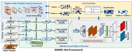
Figure 1.
The overall structure of GDMR-Net Framework.
3.1. Lightweight Backbone Network
In order to obtain a neural network model with good performance in this scenario, it is usually necessary to perform complex feature extraction and information fusion on the input data. Since the discriminative regions in fine-grained categories are hidden in subtle locations, we firstly utilize a relatively robust network with small-scale parameters to extract enough features by constraining the size and stride of the convolutional filters and pooling kernels. The truncated cross stage partial network (CSPNet) [57] is designed as the backbone network to extract coarse-granulometric features, which strengthen the learning ability of classical CNN approaches, so that they can maintain sufficient accuracy while becoming lightweight. The detailed architecture of our proposed CSPXNet is as shown in Figure 2, consisting of an input block, four CSPX Stage blocks, and an output pooling block.
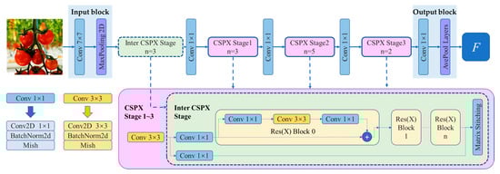
Figure 2.
Network structure description of the CSPXNet network.
Considering that the images collected have different pixel sizes and data storage formats, including jpg, png, and tif, these factors should be fully considered before designing the input module of the entire model. Thereby, the input block contains a convolutional kernel of 7 × 7 with a step size of 2, and a maximum pooling layer with a kernel of 2 × 2, of which step size is 2. It then passes through the inter CSPX stage consisting of n partial residual blocks and a partial transition layer. The feature maps of the base layer in the inter CSPX stage are split into two parallel paths. Path b first passes through a convolutional layer with a convolutional kernel of 1 × 1 and a step of 1, and then passes through several residual blocks, which can be either ResNet or ResNeXt. The input of path 2 is directly summed with the result of path 1 to obtain the output of path b. Path c similarly goes through a convolutional kernel of 1 × 1 with a step size of 1 and an output of 64 channels, which is then spliced directly with the output of path b and goes through a convolutional kernel of 1 × 1 to obtain an output of 256 channels. The dimensions of all outputs will be doubled. The formulae in each CSPX stage are shown below:
where is the input of the CSPX stage, indicates the lower sampling layer, , and are the output of related lower sampling layers, represents the convolutional layer through path b and path c, respectively. represents the input of the 0th residual block, and represents the output and input of the i-th residual block. represents the inputting residual calculation. indicates that and are spliced in the channel dimension. The number of residual blocks in the four CSPX stages is . Then the pooling layer uses the global average pooling (GAP) to form the output of the backbone network, which actually represent the coarse-granulometric feature maps in the 2048-dimensional vector as follows:
where denotes all layers of the backbone network and is the input images. And the Mish function is selected as the activation function.
3.2. Higher-Order Graphic Feature Extractor
With the above backbone network, we can extract the feature map with multiple discrimination parts, which can be processed by a down-sampling operation. However, the feature map is still a high latitude matrix, which embeds the low margin into the full connection layer, leading to many learnable parameters for training. At the same time, different crops have certain hidden information in spatial distribution and shape laws, which are obviously worth exploiting to enhance the identification performance.
To facilitate strengthened performance in fine-grained representation, we introduced the graph-related convolution network to learn the higher-order semantics between different discrimination parts. Considering the graphic nodes do not exist in isolation, we used this network to build the edge associations among different sampling parts and nodes as an adjacency matrix. Through node extraction and edge construction, the higher-order features between discriminated parts are implicitly learned by spreading on graph convolution networks.
Inspired by [58], we designed a higher-order graphic extractor to exploit the discrimination aspects from the coarse feature maps, which focused on the graphic relationship carding with the discrimination response layer. The network framework is shown in Figure 3. Specifically, a convolution layer and a sigmoid function are combined to learn discriminative probability maps , which express the impact of discriminative regions on the final classification. is the channel number of the feature maps. Then, each selected patch will be assigned a corresponding discrimination probability value . The formulation is as follows:
where are coordinates of each patch, denotes the discrimination probability value of the i-th row, j-th column, and k-th channel.
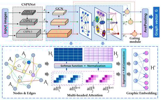
Figure 3.
The architecture of the higher-order graphic extractor framework.
After sampling operation, a discriminant feature library can be constructed as , which represents a graphic topology with nodes of the channels. These nodes share much information, so we can use the graph convolution network to aggregate these features. The relationship of adjacent pairs can be defined as:
where denotes the convolution for dimension transformation, and the last adjacency matrix is defined by self-circulating , and is an identity matrix. Through this similarity aggregation, the update paradigm of each node is as follows:
where is the learnable graph weight with a dimension . is the diagonal matrix for min-max normalization. denotes the converged matrix of . LeReLu represents a nonlinear activation function, LeakyReLU, with a well-valued negative semi-axis slope. In this way, the graph association information for each node can be continuously updated.
At the same time, another procedure aims to complete the graphical embedding for the contextual learning of massive discrimination parts. After transforming the middle features of CSPX stage 1~3 into higher-order graph features, self-attention is subsequently introduced to embed the association information between the target node and all neighbor nodes. In order to effectively assign weights among each node, function combined with normalization is utilized to calculate the attention correlation coefficient between the i-th and j-th nodes as follows:
where represents the total number of embedded graph nodes. We perform a multi-head attention mechanism to stabilize the learning process of self-attention without feature decomposition or other matrix operations. The attention coefficient is used to calculate the weighted vector of neighbor nodes passing a number of parallel attentions. The adjusted feature vector of each node is expressed as the following paradigm:
where k represents the k-th component of the multi-head attention module, where the maximum number is K. W1 represents the weight matrix, which regulates the response of different components of multi-headed attention correspondence to each adjacent node. indicates the sigmoid activation function. W2 is the learnable parameter weight and b is the mapping bias.
Thereby, the embedding process of graphic groups can efficiently allocate a high-order feature library in low-dimensional manifolds, covering the map channel dimension and node dimension at the same time. After iterative training, the message of each node is propagated in the graph structure, thus obtaining the final high-order state of all nodes. Subsequently, massive graphic features are fused through the gating module on the basis of GMP to suppress non-associated information under the guidance of graph knowledge. The variable G is defined as the obtained graphic feature map, which is prepared as input for subsequent modules and operations.
3.3. BRGAtt-Based Object Detector Network
On the basis of completing the backbone network and graph feature extractor, we further redesigned the detector network. Considering the excellent performance of the YOLO series models in object detection, this article improves the detector section of YOLOv7 [12], including the neck module with pyramidal structure, and the head module, decoupling classification and location indicators. The detailed structure illustration of the proposed detector is shown in the Figure 4.
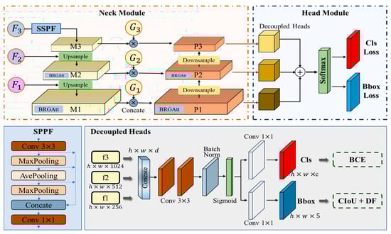
Figure 4.
The structure of the BRGAtt-based detector module.
First, design the neck module under the spatial pyramid pooling structure. It consists of bidirectional pyramid structures, top-down flow, and bottom-up flow. The inputs are the middle feature groups extracted from three CSPX stages of backbone network, covering the deep feature F3 (pass through the space pyramid pooling of SPPF structure), mid-level feature F2, and shallow feature F2, respectively. Both the top-down flow and the bottom-up flow consist of three bottleneck layers, [M1, M2, M3] and [P1, P2, P3], respectively. Adjacent bottleneck layers are connected through Up sample layers or Down sample layers according to feature dimension matches. Additionally, there are some operations such as Split and concat which incorporate with the convolution layer and the ResnetBottle layers in those bottleneck layers. In particular, we enhanced the information richness between the top-down flow and bottom-up flow by adding the graphic feature maps [G1, G2, G3] extracted from the graphic feature extractor. The result is a new aggregated feature group [f1, f2, f3], as input to the subsequent head module.
Then, the original head module has been adjusted to the decoupled head’s structure, which separates the classification prediction and Bbox regression. In fact, there have always been differences between the two tasks. Classification pays more attention to which category of the extracted features are most similar to the existing categories, while Bbox regression pays more attention to the position coordinates of the real annotation box. Therefore, if the same feature map is used for classification and positioning, the prediction accuracy will be affected to a certain extent. In the decoupling heads, three groups of new aggregated features are unified through a 1*1 convolution for dimensionality reduction, and then passed through 3 parallel branches for differential feature encoding. Each parallel branch contains two 3*3 convolution layers, a batch-norm layer with sigmoid activating, and 2 separated 1*1 convolution layers, which finally output the score vector representing the number of categories as well as the prediction box information. The loss calculation adopts the distribution focal (DF) loss combined with CIoU loss as the boxing regression loss and introduces the binary cross-entropy (BCE) loss to handle the classification task in the task-aligned-assigner tool. After decoupling, different branches are oriented to different tasks, which not only improves the model detection performance, but also greatly improves the model convergence speed.
In order to enhance the detector’s focus on fine-grained features, we introduced a new attention mechanism by effectively merging bi-level routing attention (BRA) [59] with ghost convolution, namely BRGAtt, offering better global context perception. The primary objective of the self-attention mechanism is to enhance the network’s concentration on pivotal areas. Unlike other attention modules, the BRGAtt module is designed with the query-aware sparse concept, aiming to select the relevant key-value pairs according to each query. This module starts with exploiting the least pertinent key-value pairs at the area level, thereby retaining less numerous routing regions. Subsequently, fine-grained label-to-label attention is employed to prompt these routing regions. After some matrix multiplication and ghost convolutions, BRGAtt has achieved the global perceptual performance while ensuring high computational efficiency, as show in Figure 5.
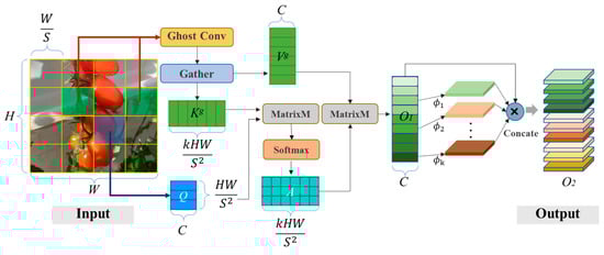
Figure 5.
The structure of the BRGAtt module.
To be more specific, input the feature map , then the BRGAtt module divides it into non-overlapping regions, where each region contains feature vectors. Thereby, the feature map X is reshaped as . The linear projection of query Q, key K, value V is calculated as follows, with their respective weights being , and :
On the basis of the first step, the area-to-area routing relationship is represented by constructing a directed graph. Apply the mean of each region to query and key, reaching the and . Calculate the adjacency matrix between two regions, indicating the degree of semantic correlation. Next, only the top k connections of each region are flited to from the directed graph relationship. Specifically, the routing index matrix is utilized to remain the indexes of each top connection:
With the regional routing index matrix , we further apply the fine-grained label to complete the token-to-token attention. For each query token in region i, all key-value pairs lie in the set of k routing regions. Thereby, use the operation to collect the key and value tensors as follows:
where and are the tensor vectors of the aggregated key and value. Use the Softmax function to complete the attention calculation on the aggregated key-value pairs. In addition, the local context enhancement (LCE) [60] function is also introduced to improve the context representation of each value with depth-wise separable convolution, of which convolution kernel size is set to 5. And the output result is expressed as follows:
Considering that the dense, small targets often congregate within specific areas of agricultural vision, it is necessary to generate more attention maps with fewer parameters to further strengthen the detector’s focus on fine-grained features. So, we introduce the ghost convolution operation through a small number of linear transformations and depth-wise conventional layers, thereby effectively reducing the computational consumption while ensuring the model’s performance. After this process, the BRGAtt module can eliminate the channels that interfere with each other so that they obtain a more comprehensive representation of the fine-grained information, leading to improved performance in small-scale object detection. The updated expression of output vector is as follows:
3.4. Rotated Annotation Optimization
To prompt the detection performance of different-oriented objects while disregarding irrelevant background information, the eight-parameter method is adopted to represent rotated bounding boxes. Each rotated rectangle is represented with 4 vertices (x1, y1), (x2, y2), (x3, y3), and (x4, y4) in a counter-clockwise order, starting from the top-left corner in the form of 8 parameter annotations. These eight parameter annotations are fed into the process of bounding box decoding to extract the rotation angle, described as the following expression:
Subsequently, the annotation format of each bounding box is transformed to . However, this angle-based rotation detection representation is troubled by issues such as angle periodicity and boundary discontinuity. Thereby, the angle regression approach is converted into a classification form to avoid the definition of angles beyond their valid range, inevitably resulting in a significant loss of accuracy. In this study, we introduce the circular smooth labels (CSL) [61] method to measure the distance between angle labels in order to mitigate the boundary discontinuity. The window function is defined to measure the angular distance between predicted and confidence labels. Within a specific range, the closer the detection value is to the ground truth, the smaller the corresponding prediction loss. The CSL expression is as follows:
where represents the original label, and denotes the window function with a controlled radius r. This radius determines the angle of the current bounding box. Consequently, as the predicted and true values become closer within a certain range, the loss value decreases. Moreover, we address the issue of angular periodicity by incorporating periodicity, whereby angles like −90 degrees and 89 degrees are considered neighbors, which exhibits higher tolerance to adjacent angles. The regression process for rotating bounding boxes with circular smooth labels is illustrated in Figure 6.
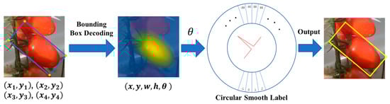
Figure 6.
Illustration of rotated annotation regression.
3.5. Loss Function Design and Setups
In order to complete the effective training of the whole model and each module, we design a new loss function to oppress the proposed GDMR-Net framework to constantly approach the global optimal result. The loss function mainly consists of 3 components: the classification prediction, the Bbox regression, and innovation module trainings. On the one hand, it is necessary to ensure the accurate identification and proper orientation of the final results. So, we follow the prevailing design philosophy. In the classification branch, we still utilize the binary cross-entropy (BCE) loss to complete the multi-label sorting task. And in the Bbox regression branch, we employ the distribution focal (DF) loss and the CIoU loss to conjointly complete the regression analysis of massive horizontal bounding boxes. This combination helps to improve the recognition ability of the model for some convenient and fuzzy targets, with probability distribution to solve the problem of unclear boundary.
As to the matching strategy, we use the task-aligned-assigner tool, which is responsible for selecting positive samples on the basis of the weighted scores of classifications and regression. To effectively remove redundant candidate boxes, the non-maximum suppression (NMS) is obtained to effectively improve the recall rate of box regression. Considering the traditional NMS algorithm is troubled by the missing overlapping objects, we adopt the soft-NMS approach to restrict the overlap basis among adjacent detection frames. When there is a high overlap with the detection box M, it is set to fractional attenuation instead of directly setting it to zero. The higher the overlap, the more serious the corresponding fractional attenuation. The expression of soft-NMS is shown as follows:
On the other hand, considering the introduction of many innovative modules, it is necessary to coordinate the learning process of gradient transfer among each module in order to achieve the end-to-end training of the entire model. Thereby, we focus on the two most important modules, and add their loss functions into the overall loss function. For the higher-order graphic feature extractor, we select its own Softmax function to supervise graph node coding and topological relationship mining. As for the rotated annotation optimization process, we also utilize the BCE loss function to facilitate the learning process of angular CSL labels. Under the supervision of this loss, the model acquires the ability to identify rotating objects effectively, considering their periodic nature and angular practices. The expression is as follows:
The aforementioned loss functions are weighted by a specific weight ratio, and the final loss function of our proposed GDMR-Net is expressed as follows:
In this context, and indicate the distribution focal loss and CIoU loss, respectively, in charge of horizontal bounding box regression. indicates the binary cross-entropy loss, responsible for the fine-grained category classification. denotes the confidence loss of higher-order graphic feature extractors, and represents angular bounding box regression. Through the monitoring of new loss, the proposed framework can not only accurately identify the categories of fine-grained crops but can also locate horizontal and rotated objects at the same time, which provides powerful performance to better meet various practical tasks in smart agricultural applications.
Throughout the training process, distinctive learning rates are assigned to individual modules. The uniform sampling branch is fine-tuned using a base learning rate of 0.005, and each module’s classifier is trained from scratch with a learning rate of 0.1. All network parameters are optimized using an SGD optimizer with corresponding momentum of 0.943 and weight decay values of 0.0005. On one hand, the optimizer can dynamically turn on or off the adaptive learning rate based on the potential scatter of the variance, providing a dynamic warm-up without the need for adjustable parameters. On the other hand, the lookahead operation can be seen as an external attachment to the optimizer by saving two sets of weights, fast and slow weights.
For initialing the parameters, we use the default settings with the initial batch size set at 256, and the input image size set to 640 × 640. The EMA decay is set to 0.999. The training duration spans 450 epochs, employing a cosine annealing algorithm with restart activation to learning rate reduction. The learning rate is adjusted to 50% of its initial value from the preceding cycle after each restart. The cosine annealing step is defined as 2, and each stage’s base cycle length is set to 10 cycles. Consequently, the learning rate is reset at the 51st, 101st, 201st, and 351st cycles for improved optimization. Moreover, the data augmentation includes the rotation, translation, brightness enhancement, Gaussian blur, and CutMix, among others. In particular, it stops the Mosaic augmentation in the final 10 epochs, similar to the method proposed in YOLOX models. Finally, the backbone network is pre-trained on the large-scale ImageNet dataset, and other modules are then trained on the MSCOCO dataset, before transferring to validation experiments on crop identification and detection datasets.
4. Experiments and Discussions
4.1. Experimental Devices and Dataset Collection
The collection of the experimental dataset in this study was carried out in the Beijing Chaolai Agronomic Garden. As shown in Figure 7a, considering the engineering applicability of the algorithm, we placed some cameras (device type: Intel RealSense D435i camera) on the picking robot to collect the crop image dataset and verify model performance. As shown in Figure 7b, the row spacing in the greenhouse was 1.9 m, the spacing between adjacent plants was 0.2 m, and the width of the robot was 0.8 m. During the robot operation, the travel speed of the robot on the track was set to 0.4 m/s. The sample of the collected pictures is shown in Figure 7c. Meanwhile, we also used some smartphones and surveillance cameras to collect images of different crops and add them to the database. Each device uploads pictures of crops to the cloud server via CAN or wireless fidelity. In order to facilitate the subsequent model training and practical application, we set up the automatic cropping function to unify the image sizes from different sources to 1000 × 1000 pixels. Those collected data were submitted to the cloud platforms, and combined with plant cultivation rules and regulations, to determine management measures.
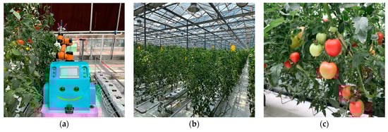
Figure 7.
The data collection process via picking robots in the greenhouse environment.
Through the use of various devices and pieces of equipment, the crop dataset has collected over 21,600 images, including vegetables and fruits in intelligent greenhouses. Currently, the dataset covers vegetables and fruits of 19 upper-level categories and 31 subordinate classes, which are the most reasonable for the PA purpose, and arranges crops into root vegetable, cabbage, leafy vegetable, melon, fruits, etc. Moreover, each crop species contains sufficient images with different plant tissues, photography angles, focal lengths, and rotating resolutions. The construction principles guide the process of image collection, as well as the detail quantity of images and annotated samples. Images with fine-grained characteristics are challenging to subsequent deep learning models learning precise detection. Thus, it is worth monitoring the growth and healthy status of crops and improving the decision-making efficiency of smart agricultural management.
To ensure the reliability of the training, we randomly divided the dataset into a training set and a validation set in an 8:2 ratio. We built a cloud server platform with Ubuntu 20.04LTS, which consists of a dual-core Intel Xeon E5-2690 V3@2.6 GHz × 48 processor, 128 G RAM and 2 × 2 T SSD, 8 NVIDIA Tesla p40 GPUs for graphics, and 168 G computational cache. All the codes and experiments are based on the deep learning framework Pytorch 1.7.1 and TensorFlow2.4.0 under the Python 3.8.2 programming environment.
4.2. Evaluation Indicators
To supervise a model’s training process, the , , and are selected as indicators to evaluate the model’s performance. Among them, True Positive (TP) means that the predicted result and ground truth are positive samples. False Positive (FP) indicates that the detected result is negative, but the predicted result is true. False Negative (FN) means that the detected result is positive instead of negative. True Negative (TN) is the predicted result and the ground truth are a negative sample. The calculation function of three indicators is as follows:
In particular, the is the percentage of recognized images (batch size) correctly identified, is the ratio of correctly identified targets to all targets in the test set, and is used to evaluate the model’s performance balance between the weights of and . Moreover, a curve plotted for each category based on the recall and precision is introduced to further evaluate the detection performance of multiple-category objects. Here, AP is the area under the curve, and mAP is the average of the multiple categories of APs. In this study, we used the mAP to evaluate the trained model. Additionally, the average recognition time (ART) represents how long the trained model needs to handle a single image and recognize different samples in the testing stage. Obviously, the smaller the ART value, the better the efficiency modeling performance in recognizing a single image for agricultural practices. The function of mAP and ART are shown as follows:
4.3. Comparative Experiment Results
In order to verify the detection performance of the proposed GDMR-Net, this paper conducts comparative experiments on collected crop datasets, and selects two-stage deep learning algorithms Cascade R-CNN [62], Sparse R-CNN [63], PANet [36], and CenterNet [64] for comparison, and selects single-stage algorithms such as Yolov3 [38], Yolov4 [39], Yolov5 [40], YoloX [41], Yolov6 [42], and Yolov7 [12] as methods for comparison. During their training and testing processes, the data and type formats remain consistent with our proposed methods in this article. The evaluation indexes selected in this paper were AP average accuracy value and AP50 (IOU > 0.5) accuracy value. The detection results of different models are shown in Table 1.

Table 1.
Comparative detection results of different models.
The accuracy values of mAP and AP50 of all the models are listed. Compared with other advanced models, it shows that our proposed approach has achieved comparable or better results for fine-grained crop detection. We first observed that the accuracy results of anchor-free models are generally better than anchor-based models on the agricultural dataset. Thereby, additional annotation information does help improve the performance of detection models. For instance, CenterNet employs the center points for anchor-free object detection with the mAP to 76.8%, surpassing two-stage algorithm models such as Cascade R-CNN (60.2%), Sparse R-CNN (65.8%), PANet (70.4%), and RetinaNet (76.7%).
At the same time, we can see that CenterNet’s results are still not compared to the results of the YOLO series models, which means that in complex agricultural scenes, it is difficult to obtain additional information about handling with automatic crop recognition. Thereby, drawing inspiration from the performance enhancements brought about by CSPNet in the YOLO series, our proposed GDMR-Net also incorporates a CSPXnet50 design. It achieves a mAP up to 89.6% in the detection accuracy of fine-grained crop species, representing a 1.2% improvement over ResNet50. Compared to the state-of-the-art method YOLO-v7, our detection performance significantly improved by at least 1.5%. Similarly, in the evaluation indicator of AP50, our method also achieved the best results, 94.7%, an improvement of 1.6% over the best YOLO-v7 model. It is worth noting that the proposed GDMR-Net does not increase the number of model parameters improving the identification accuracy, even though it has more parameters than Sparse R-CNN, Yolov3, Yolov4, and Yolov5 models. Compared with Yolov7, which has a higher performance, the parameter number of GDMR-Net is reduced by almost 160 Mbyte. So, it is certain that our proposed method has achieved a good balance between identification accuracy and model parameters, which is suitable for practical applications.
More comparisons of precision histograms in terms of different models are provided in Figure 8, which can further illustrate the feasibility and effectiveness of proposed GDMR-Net (CSPXnet50 backbone). As the average precision values of each model for all crop categories depicted in the figure, our proposed method obtains the highest mAP value and AP50 value (89.6% and 94.7%, respectively). Even under the ResNet50 backbone without lightweight optimization, our GDMR-Net still obtained better results than other methods, achieving mAP values up to 88.4%, as well as AP50 values up to 93.8%. The intuitive comparison results of each model indicate that the higher-order graphic features with BRGAtt-based attention mechanisms have a great influence on the fine-grained learning of local and global information during the crop detection.
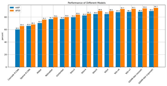
Figure 8.
Comparison performance of each model.
To test the model’s convergence effect, we further developed the comparable experiments to analyze the value change of loss functions among different methods. The loss function was used to estimate the degree of inconsistency between the predicted result of the models and the true label. The smaller the loss function, the better the robustness of the model. As shown in Figure 9, we observed that the general trend of each model’s loss curve is decreasing and approaching a steady state after 45 updated epochs. Among them, the loss functions of YOLO series models generally had smaller loss function values with faster speed of convergence processes. In contrast, the loss curves of our proposed models achieved better performance, and the convergence process was stabilized very quickly near the 10th epoch. Therefore, the GDMR-Net’s robustness was trustworthy to handle the fine-grained crop detection, which offers great potential in enhancing smart agriculture management and food supply security in actual complex scenarios.
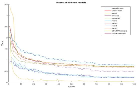
Figure 9.
Loss value curves of each model.
To demonstrate the practical performance of our proposed model, we randomly selected some real-world images to test the model’s capabilities. We also conducted performance result visitation compared with other state-of-the-art models. As shown in Figure 10, to verify the detection performance of different models, we selected 8 image samples containing different categories for testing. These results show that the proposed method has good fine-grain identification ability for crops of different scales and categories and can accurately detect the corresponding quantity and location information. For example, the strawberries, apples, and small tomatoes shown in Samples 1, 2, and 7 all have multiple objects in a single photo and are generally smaller in size. Other models often have missing detection or inaccurate positioning, but our method can effectively avoid the above cases, thus proving the stability and accuracy of our method. At the same time, for crops with mutual occlusion or background occlusion, such as oranges, tomatoes, and grapes in Samples 3, 5, and 6, other methods are often unable to be deduced more accurately in frame regression, resulting in a discrepancy between the predicted size and the actual result. However, our method can effectively alleviate this problem, revealing its better immunity to the occlusion issue. Therefore, this shows that our model completes the inspection of crops in agricultural scenarios such as greenhouses, and that our model has unique advantages over other models in occlusion and dense distribution scenarios.
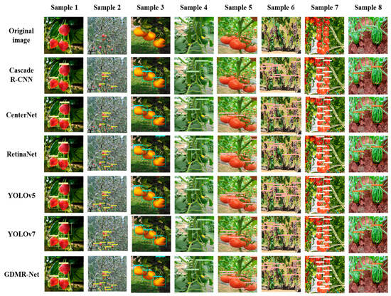
Figure 10.
The normal crop detection results of different models.
4.4. Ablation Analyses and Discussion
To validate the effectiveness of the individual modules of GDMR-Net, this paper conducted ablation experiments, and the results of the ablation experiments are shown in Table 2. (Where, A: CSPXnet, B: graph-related higher-order feature extractor, C: multi-crossed ghost attention module, D: rotated annotations).
Table 2.
Ablation results of each module.
In this section, we develop some ablation comparison experiments to demonstrate the effectiveness of the proposed method. Table 2 shows the comparative ablation experiments for the proposed GDMR-Net. The first line represents the detection performance of the original model (YOLOv5) on the dataset, achieving an accuracy of 84.8% mAP and 89.8% AP50, demonstrating a good baseline detection performance. Adding the new backbone CSPXnet to the original model can improve the accuracy by 2.8% and can improve the mAP by 2.8% without any computational process, which indicates that the proposed backbone network in this paper can easily extract richer features. Then, adding the graphic feature extractor can also improve the mAP by 3.3%, Furthermore, sequentially adding the BRG attention module and rotated annotations leads to a 0.3% and 0.6% increase in mAP, respectively, indicating that these three modules can effectively cooperate, fully utilizing the feature information provided by the backbone network without significantly increasing the parameter count, and maintaining high detection speed. Therefore, it can be concluded that our model is better suited for fine-grained crop identification and detection tasks. To assess the impact of different attention mechanisms on network performance, we employed the CNN component to propagated images, computed raw scores for specific categories, and backpropagated gradients, generating Grad-CAM localizations (heatmaps). Figure 11 presents heatmaps for networks using various attention mechanisms. GDMR-Net with the CBAM attention block exhibits a concentrated region of interest over the target area, demonstrating strong detection capabilities.
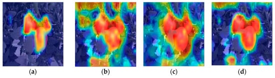
Figure 11.
(a) The heatmap of YOLOv5 + Ghost_Convolution; (b) The heatmap of GDMR-Net + SE; (c) The heatmap of GDMR-Net + CA; (d) The heatmap of GDMR-Net + CBAM.
As shown in Figure 12, the red rectangular box represents ripe tomatoes. Detecting tomatoes in a greenhouse environment is often challenging when leaves and fruits overlap. We can see a missed detection of tomatoes in the detection results of (a) +B, (b) +B+C, (c) +B+C+D, and (d) +A+B+C. However, GDMR-Net shows an excellent capability for small-target detection, as show in Figure 12e. It can be clearly seen that our method has better target detection performance under full state transformation after different submodules cooperate with each other, especially for small targets and overlapping objects with better fault tolerance.
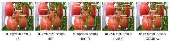
Figure 12.
The detection result of different models.
To further illustrate the performance of our model, we plotted the confusion matrix of the accuracy rates of the three models, as shown in Figure 13. Our model has a high accuracy rate on each class on the cassava dataset with the best effect. The worst is the third category, but the accuracy rate also reached 95%, and the best impact is the 0th category. Moreover, we achieved the spatial location detection of tomato objects by combining GDMR-Net with Intel RealSense D435i. In an actual greenhouse environment, the camera inevitably shoots the targets in the back row through the gaps in which the plants grow. From the perspective of actual picking tasks, the robotic arm could only pick tomatoes in the current row. It is not practical to detect all targets in the scene. In contrast, too many national standards will increase the amount of model calculation and reasoning time.
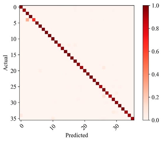
Figure 13.
Confusion matrix.
To minimize the impact of the complex greenhouse environment on target recognition and the final picking effect, we filtered all video streams over 1.5 m so that the vision algorithm only focused on the recognition and detection of targets within a range of 1.5 m, as shown in Figure 14. It can be seen that the proposed GDMR-Net method effectively alleviates many vital issues in fine-grain crop target detection. These results show that the proposed model not only has the potential to be applied to distributed networks and multi-processor embedded systems [65], which also has good guiding significance for improving multi-intelligence collaborative operations [66]. This further verifies that this method has good application value.
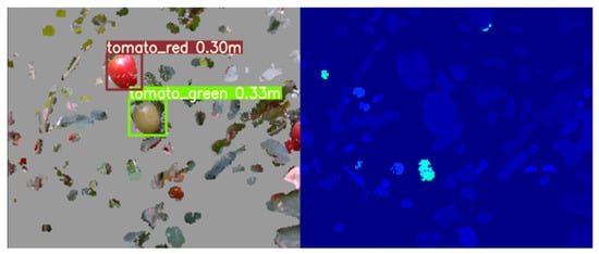
Figure 14.
The tomato detection within a range of 1.5 m.
5. Conclusions
Strengthening the visual inspection performance is of great significance to improve the intelligence of smart agriculture and ensure the food supply’s cyber security. Currently, the existing deep learning technology generally lacks the effective ability to deal with crop detection with rotating postures and fine-grained characters. In order to address those issues, we proposed a novel graph detection neural network combining graph representation and multi-crossed attention techniques, namely GDMR-Net, which is applied to fine-grained crop detection and recognition tasks in smart agriculture management and supply security. Specifically, the overall structure of GDMR-Net is divided into four major components: a light-weight CSPXNet Backbone, graph feature extractor, BRGAtt-based-object detector, and optimized loss function. With the input of massive crop images collected from different IoT devices and cameras, we first utilized the truncated-cross stage partial-network (CSPNet) as the backbone network to accurately extract abundant feature maps under multiple granularities and dimensions. Some lightweight techniques are introduced to compress the overall parameters of the model and optimize the network structure. Then, the higher-order graphic feature extractor is designed to comprehensively observe the fine-grained features and potential graphic relationships among massive crops, enabling better perception capabilities of agricultural robots adapted to complex environments. Subsequently, we enhanced the decoupling of neck and head modules by addressing bilevel routing ghost attention with the rotation annotations, leading to a redesigned detector network. This is proposed to handle continuous posture changes during crop growth and mutual occlusion. Finally, to coordinate the information interaction between the entire network and each module, we devised a novel loss function to guide the proposed framework towards approaching the global optimal result of both detection and classification tasks.
In order to verify the effectiveness of this proposed approach, an extensive set of experiments were implemented on a practical agricultural dataset. Compared to existing advanced deep learning and machine-learning methods, the proposed GDMR-Net achieved preferable performance in crop detection and identification, with a mAP accuracy of 89.6% and an AP50 accuracy of 94.7%, respectively. Moreover, some ablation studies further proved the good stability and robustness of the proposed method, of which the parameter size is only 62.8 Mbyte while maintaining a high processing speed of 89 frames per second. This shows that the proposed approach has achieved a good balance in identification accuracy, parameter scale, and processing timeliness, which is more suitable for the complex applications of smart agricultures and food supply security.
Of course, our proposed method still has some limitations, lacking more complex scenarios and requiring further performance improvement. Thereby, we will continue to focus on model structure optimization and data scaling to further enhance the usefulness and recognition performance on a variety of real-world devices and scenarios. In future work, relevant technologies will be studied to expand the application scope of this model in smart agriculture and the food supply chain. They can also be applied to other fields, such as time prediction, signal modelling, and control systems.
Author Contributions
Conceptualization, Z.X.; methodology, Z.X. and J.K.; software, Z.X. and X.Z.; validation, Y.X.; formal analysis, Z.X.; investigation, C.H.; resources, C.H.; data curation, X.Z.; writing—original draft preparation, Z.X. and X.Z.; writing—review and editing, J.K.; visualization, C.H.; supervision, J.K.; project administration, J.K.; funding acquisition, J.K. All authors have read and agreed to the published version of the manuscript.
Funding
This work was supported in part by the National Key Research and Development Program of China (No. 2021YFD2100605), the National Natural Science Foundation of China (No. 62173007, 62006008), and the Project of Beijing Municipal University Teacher Team Construction Support Plan (No. BPHR20220104).
Data Availability Statement
Please contact the corresponding author for data available.
Conflicts of Interest
The authors declare that there are no conflict of interest regarding the publication of this paper.
References
- Sinha, B.B.; Dhanalakshmi, R. Recent advancements and challenges of Internet of Things in smart agriculture: A survey. Future Gener. Comput. Syst. 2022, 126, 169–184. [Google Scholar] [CrossRef]
- Kong, J.; Fan, X.; Jin, X.; Su, T.; Bai, Y.; Ma, H.; Zuo, M. BMAE-Net: A Data-Driven Weather Prediction Network for Smart Agriculture. Agronomy 2023, 13, 625. [Google Scholar] [CrossRef]
- Kin, M.; Eyduran, S.P.; Eyduran, E.; Reed, B.M. Analysis of macro nutrient related growth responses using multivariate adaptive regression splines. Plant Cell Tissue Organ Cult. PCTOC 2020, 140, 661–670. [Google Scholar]
- Wang, F.; Sun, Z.; Chen, Y.; Zheng, H.; Jiang, J. Xiaomila Green Pepper Target Detection Method under Complex Environment Based on Improved YOLOv5s. Agronomy 2022, 12, 1477. [Google Scholar] [CrossRef]
- Li, H. A Visual Recognition and Path Planning Method for Intelligent Fruit-Picking Robots. Sci. Program. 2022, 2022, 1297274. [Google Scholar] [CrossRef]
- Cho, S.; Kim, T.; Jung, D.H.; Park, S.H.; Na, Y.; Ihn, Y.S.; Kim, K. Plant growth information measurement based on object detection and image fusion using a smart farm robot. Comput. Electron. Agric. 2023, 207, 107703. [Google Scholar] [CrossRef]
- Qi, T.; Xie, H.; Li, P.; Ge, J.; Zhang, Y. Balanced Classification: A Unified Framework for Long-Tailed Object Detection. IEEE Trans. Multimed. 2023. [Google Scholar] [CrossRef]
- Badrinarayanan, V.; Kendall, A.; Cipolla, R. Segnet: A deep convolutional encoder-decoder architecture for image segmentation. IEEE Trans. Pattern Anal. Mach. Intell. 2017, 39, 2481–2495. [Google Scholar] [CrossRef]
- Nan, Y.L.; Zhang, H.C.; Zeng, Y.; Zheng, J.Q.; Ge, Y.F. Intelligent detection of Multi-Class pitaya fruits in target picking row based on WGB-YOLO network. Comput. Electron. Agric. 2023, 208, 107780. [Google Scholar] [CrossRef]
- Du, L.; Zhang, R.; Wang, X. Overview of two-stage object detection algorithms. J. Phys. 2020, 1, 1544. [Google Scholar] [CrossRef]
- Fan, J.; Huo, T.; Li, X. A Review of One-Stage Detection Algorithms in Autonomous Driving. In Proceedings of the 2020 4th CAA International Conference on Vehicular Control and Intelligence (CVCI), CVCI 2020, Hangzhou, China, 18–20 December 2020; pp. 210–214. [Google Scholar] [CrossRef]
- Wang, C.Y.; Bochkovskiy, A.; Liao, H.Y.M. YOLOv7: Trainable bag-of-freebies sets new state-of-the-art for real-time object detectors. In Proceedings of the IEEE/CVF Conference on Computer Vision and Pattern Recognition, CVPR 2023, Vancouver, BC, Canada, 17–24 June 2023; pp. 7464–7475. [Google Scholar]
- Wilbert, M.R.; Vicente, M.; Nieves, M.; Simón, I.; Lidón, V.; Fernandez-Zapata, J.C.; Martinez-Nicolas, J.J.; Cámara-Zapata, J.M.; García-Sánchez, F. Agricultural and Physiological Responses of Tomato Plants Grown in Different Soilless Culture Systems with Saline Water under Greenhouse Conditions. Sci. Rep. 2019, 9, 6733. [Google Scholar] [CrossRef]
- Lu, Y.; Young, S. A survey of public datasets for computer vision tasks in precision agriculture. Comput. Electron. Agric. 2020, 178, 105760. [Google Scholar] [CrossRef]
- Xu, L.; Zhang, K.; Yang, G.; Chu, J. Gesture recognition using dual-stream CNN based on fusion of sEMG energy kernel phase portrait and IMU amplitude image. Biomed. Signal Process. Control 2022, 73, 103364. [Google Scholar] [CrossRef]
- Ta, H.T.; Rahman, A.B.S.; Najjar, L.; Gelbukh, A. GAN-BERT: Adversarial Learning for Detection of Aggressive and Violent Incidents from social media. In Proceedings of the Iberian Languages Evaluation Forum (IberLEF 2022), CEUR Workshop Proceedings, Jaén, Spain, 20–21 September 2022; Available online: https://ceur-ws.org (accessed on 20 September 2022).
- Wang, J.; Li, X.; Li, J.; Sun, Q.; Wang, H. NGCU: A new RNN model for time-series data prediction. Big Data Res. 2022, 27, 100296. [Google Scholar] [CrossRef]
- Chen, J.; Chen, X.; Chen, S.; Liu, Y.; Rao, Y.; Yang, Y.; Wang, H.; Wu, D. Shape-Former: Bridging CNN and Transformer via ShapeConv for multimodal image matching. Inf. Fusion 2023, 91, 445–457. [Google Scholar] [CrossRef]
- Zheng, Y.Y.; Kong, J.L.; Jin, X.B.; Wang, X.Y.; Zuo, M. CropDeep: The crop vision dataset for deep-learning-based classification and detection in precision agriculture. Sensors 2019, 19, 1058. [Google Scholar] [CrossRef] [PubMed]
- Hou, S.; Feng, Y.; Wang, Z. VegFru: A Domain-Specific Dataset for Fine-Grained Visual Categorization. In Proceedings of the IEEE International Conference on Computer Vision, ICCV 2017, Venice, Italy, 22–29 October 2017; pp. 541–549. [Google Scholar] [CrossRef]
- Van Horn Macaodha, G. iNat Challenge 2021—FGVC8. Kaggle. 2021. Available online: https://kaggle.com/competitions/inaturalist-2021 (accessed on 8 March 2021).
- Fruits 360 Dataset. Available online: https//github.com/Horea94/Fruit-Images-Dataset (accessed on 18 May 2020).
- Zawbaa, H.M.; Hazman, M.; Abbass, M.; Hassanien, A.E. Automatic fruit classifcation using random forest algorithm. In Proceedings of the 2014 14th International Conference on Hybrid Intelligent Systems, IS on HIS 2014, Kuwait, Kuwait, 14–16 December 2014; pp. 164–168. [Google Scholar] [CrossRef]
- Zeng, G. Fruit and vegetables classification system using image saliency and convolutional neural network. In Proceedings of the 2017 IEEE 3rd Information Technology and Mechatronics Engineering Conference (ITOEC), ITOEC 2017, Chongqing, China, 3–5 October 2017; pp. 613–617. [Google Scholar] [CrossRef]
- Gurunathan, K.; Bharathkumar, V.; Meeran, M.H.A.; Hariprasath, K.; Jidendiran, R. Classification of Cultivars Employing the Alexnet Technique Using Deep Learning. In Proceedings of the 2023 International Conference on Bio Signals, Images, and Instrumentation, ICBSII 2023, Chennai, India, 16–17 March 2023; pp. 1–7. [Google Scholar] [CrossRef]
- Kausar, A.; Sharif, M.; Park, J.; Shin, D.R. Pure-CNN: A Framework for Fruit Images Classification. In Proceedings of the 2018 International Conference on Computational Science and Computational Intelligence, CSCI 2018, Las Vegas, NV, USA, 12–14 December 2018; pp. 404–408. [Google Scholar] [CrossRef]
- Mohammed, A.A.; Jaber, A.; Suleman, A. Satin Bowerbird Optimization with Convolutional LSTM for Food Crop Classification on UAV Imagery. IEEE Access 2023, 11, 41075–41083. [Google Scholar] [CrossRef]
- Kong, J.; Fan, X.; Zuo, Z.; Muhammet, D.; Jin, X.; Zhong, K. ADCT-Net: Adaptive traffic forecasting neural network via dual-graphic cross-fused transformer. Inf. Fusion 2023, 103, 102122. [Google Scholar] [CrossRef]
- Xing, S.; Lee, H.J. Crop pests and diseases recognition using DANet with TLDP. Comput. Electron. Agric. 2022, 199, 107144. [Google Scholar] [CrossRef]
- Kong, J.; Fan, X.; Jin, X.; Lin, S.; Zuo, M. A variational Bayesian inference-based en-decoder framework for traffic flow prediction. IEEE Trans. Intell. Transp. Syst. 2023, 2, 1–10. [Google Scholar] [CrossRef]
- Sengupta, S.; Lee, W.S. Identification and determination of the number of immature green citrus fruit in a canopy under different ambient light conditions. Biosyst. Eng. 2014, 117, 51–61. [Google Scholar] [CrossRef]
- Kuznetsova, A.; Maleva, T.; Soloviev, V. Using YOLOv3 Algorithm with Pre- and Post-Processing for Apple Detection in Fruit-Harvesting Robot. Agronomy 2020, 10, 1016. [Google Scholar] [CrossRef]
- Girshick, R.; Donahue, J.; Darrell, T.; Malik, J. Rich Feature Hierarchies for Accurate Object Detection and Semantic Segmentation. In Proceedings of the IEEE Conference on Computer Vision and Pattern Recognition, CVPR 2014, Columbus, OH, USA, 23–28 June 2014; pp. 580–587. [Google Scholar] [CrossRef]
- Kong, J.; Xiao, Y.; Jin, X.; Cai, Y.; Ding, C.; Bai, Y. LCA-Net: A Lightweight Cross-Stage Aggregated Neural Network for Fine-Grained Recognition of Crop Pests and Diseases. Agriculture 2023, 13, 2080. [Google Scholar] [CrossRef]
- Wang, M.; Fu, B.; Fan, J.; Wang, Y.; Zhang, L.; Xia, C. Sweet potato leaf detection in a natural scene based on faster R-CNN with a visual attention mechanism and DIoU-NMS. Ecol. Inform. 2023, 73, 101931. [Google Scholar] [CrossRef]
- Liu, S.; Qi, L.; Qin, H.; Shi, J.; Jia, J. Path Aggregation Network for Instance Segmentation. In Proceedings of the IEEE Conference on Computer Vision and Pattern Recognition, CVPR 2018, Salt Lake City, UT, USA, 18–23 June 2018; pp. 8759–8768. [Google Scholar] [CrossRef]
- Lin, T.Y.; Goyal, P.; Girshick, R.; He, K.; Dollar, P. Focal loss for dense object detection. In Proceedings of the IEEE International Conference on Computer Vision, ICCV 2017, Venice, Italy, 22–29 October 2017; pp. 2980–2988. [Google Scholar] [CrossRef]
- Redmon, J.; Farhadi, A. YOLOv3: An Incremental Improvement. arXiv 2018, arXiv:1804.02767. [Google Scholar] [CrossRef]
- Bochkovskiy, A.; Wang, C.; Liao, H. YOLOv4: Optimal Speed and Accuracy of Object Detection. arXiv 2020, arXiv:2004.10934. [Google Scholar] [CrossRef]
- Zhu, X.; Lyu, S.; Wang, X.; Zhao, Q. TPH-YOLOv5: Improved YOLOv5 Based on Transformer Prediction Head for Object Detection on Drone-Captured Scenarios. In Proceedings of the IEEE/CVF International Conference on Computer Vision, ICCV 2021, Montreal, BC, Canada, 11–17 October 2021; pp. 2778–2788. [Google Scholar] [CrossRef]
- Ge, Z.; Liu, S.; Wang, F.; Li, Z.; Sun, J. YOLOX: Exceeding YOLO Series in 2021. arXiv 2021, arXiv:2107.08430. [Google Scholar] [CrossRef]
- Li, C.; Li, L.; Jiang, H.; Weng, K.; Geng, Y.; Li, L.; Wei, X. YOLOv6: A single-stage object detection framework for industrial applications. arXiv 2022, arXiv:2209.02976. [Google Scholar]
- Wang, E.; Su, R.; Huang, B.; Lin, J. Enhancing YOLOv7-Based Fatigue Driving Detection through the Integration of Coordinate Attention Mechanism. In Proceedings of the 2023 IEEE International Conference on Image Processing and Computer Applications (ICIPCA), ICIPCA 2023, Kuala Lumpur, Malaysia, 8–11 October 2023; pp. 725–729. [Google Scholar] [CrossRef]
- Law, H.; Deng, J. Cornernet: Detecting objects as paired keypoints. In Proceedings of the European Conference on Computer Vision (ECCV,) ECCV 2018, Munich, Germany, 8–14 September 2018; pp. 734–750. [Google Scholar] [CrossRef]
- Tian, Z.; Shen, C.; Chen, H.; He, T. Fcos: Fully convolutional one-stage object detection. In Proceedings of the IEEE/CVF international conference on computer vision 2019, ICCV 2019, Seoul, Republic of Korea, 27 October–2 November 2019; pp. 9627–9636. [Google Scholar] [CrossRef]
- Bargoti, S.; Underwood, J.P. Image Segmentation for Fruit Detection and Yield Estimation in Apple Orchards. J. Field Robot. 2017, 34, 1039–1060. [Google Scholar] [CrossRef]
- Yang, R.L.; Hu, Y.W.; Yao, Y.; Gao, M.; Liu, R.M. Fruit Target Detection Based on BCo-YOLOv5 Model. Mob. Inf. Syst. 2022, 2022, 8457173. [Google Scholar] [CrossRef]
- Lu, L.P.; Li, H.S.; Ding, Z.; Guo, Q. An improved target detection method based on multiscale features fusion. Microw. Opt. Technol. Lett. 2020, 62, 3051–3059. [Google Scholar] [CrossRef]
- Shao, M.; Nie, C.; Zhang, A.; Shi, L.; Zha, Y.; Xu, H.; Yang, H.; Yu, X.; Bai, Y.; Liu, S.; et al. Quantifying effect of maize tassels on LAI estimation based on multispectral imagery and machine learning methods. Comput. Electron. Agric. 2023, 211, 108029. [Google Scholar] [CrossRef]
- Lu, H.; Cao, Z.; Xiao, Y.; Fang, Z.; Zhu, Y. Toward Good Practices for Fine-Grained Maize Cultivar Identification with Filter-Specific Convolutional Activations. IEEE Trans. Autom. Sci. Eng. 2018, 15, 430–442. [Google Scholar] [CrossRef]
- Kong, J.; Wang, H.; Wang, X.; Jin, X.; Fang, X.; Lin, S. Multi-stream hybrid architecture based on cross-level fusion strategy for fine-grained crop species recognition in precision agriculture. Comput. Electron. Agric. 2021, 185, 106134. [Google Scholar] [CrossRef]
- Li, Z.; Chen, G.; Zhang, T. A CNN-Transformer Hybrid Approach for Crop Classification Using Multitemporal Multisensor Images. IEEE J. Sel. Top. Appl. Earth Obs. Remote Sens. 2020, 13, 847–858. [Google Scholar] [CrossRef]
- Xiao, L.; Wu, X.; Wang, G. Social Network Analysis Based on Graph SAGE. In Proceedings of the 2019 12th International Symposium on Computational Intelligence and Design (ISCID), ISCID 2019, Hangzhou, China, 14–15 December 2019; pp. 196–199. [Google Scholar] [CrossRef]
- Han, Q. TrustGNN: Enhancing GNN via Multi-similarity Neighbors Identifying for Social Recommendation. In Proceedings of the 2022 IEEE Conference on Telecommunications, Optics and Computer Science (TOCS), TOCS 2022, Dalian, China, 11–12 December 2022; pp. 749–755. [Google Scholar] [CrossRef]
- Bi, K.; Xie, L.; Zhang, H.; Chen, X.; Gu, X.; Tian, Q. Accurate medium-range global weather forecasting with 3D neural networks. Nature 2023, 619, 533–538. [Google Scholar] [CrossRef]
- Wang, C.; Zhou, J.; Zhang, Y.; Wu, H.; Zhao, C.; Teng, G.; Li, J. A Plant Disease Recognition Method Based on Fusion of Images and Graph Structure Text. Front. Plant Sci. 2022, 12, 731688. [Google Scholar] [CrossRef]
- Wang, C.Y.; Liao, H.Y.M.; Wu, Y.; Chen, P.; Hsieh, J.W.; Yeh, I.H. CSPNet: A New Backbone that can Enhance Learning Capability of CNN. In Proceedings of the IEEE/CVF Conference on Computer Vision and Pattern Recognition Workshops, CVPR 2020, Seattle, WA, USA, 13–19 June 2020; pp. 390–391. [Google Scholar] [CrossRef]
- Yang, T.; Liang, J.; Pang, Y.; Xie, P.Y.; Qian, Y.H.; Wang, R.L. An efficient feature selection algorithm based on the description vector and hypergraph. Inf. Sci. 2023, 629, 746–759. [Google Scholar] [CrossRef]
- Zhu, L.; Wang, X.; Ke, Z.; Zhang, W.; Lau, R. BiFormer: Vision Transformer with Bi-Level Routing Attention. In Proceedings of the IEEE/CVF Conference on Computer Vision and Pattern Recognition, CVPR 2023, Vancouver, BC, Canada, 18–22 June 2023; pp. 10323–10333. [Google Scholar]
- Ren, S.; Zhou, D.; He, S.; Feng, J.; Wang, X. Shunted self-attention via multi-scale token aggregation. In Proceedings of the IEEE/CVF Conference on Computer Vision and Pattern Recognition, CVPR 2022, New Orleans, LA, USA, 18–24 June 2022; pp. 10853–10862. [Google Scholar] [CrossRef]
- Yang, X.; Yan, J. On the arbitrary-oriented object detection: Classification based approaches revisited. Int. J. Comput. Vis. 2022, 130, 1340–1365. [Google Scholar] [CrossRef]
- Cai, Z.; Vasconcelos, N. Cascade r-cnn: Delving into high quality object detection. In Proceedings of the IEEE Conference on Computer Vision and Pattern Recognition, CVPR 2018, Salt Lake City, UT, USA, 18–23 June 2018; pp. 6154–6162. [Google Scholar] [CrossRef]
- Sun, P.; Zhang, R.; Jiang, Y.; Kong, T.; Xu, C.; Zhan, W.; Tomizuka, M.; Li, L.; Yuan, Z.; Wang, C.; et al. Sparse r-cnn: End-to-end object detection with learnable proposals. In Proceedings of the IEEE/CVF Conference on Computer Vision and Pattern Recognition, CVPR 2021, Nashville, TN, USA, 20–25 June 2021; pp. 14454–14463. [Google Scholar] [CrossRef]
- Zhou, X.; Wang, D.; Krähenbühl, P. Object as Points. arXiv 2019, arXiv:1904.07850. [Google Scholar] [CrossRef]
- Chen, J.; Han, P.; Zhang, Y.; You, T.; Zheng, P. Scheduling energy consumption-constrained workflows in heterogeneous multi-processor embedded systems. J. Syst. Archit. 2023, 142, 102938. [Google Scholar] [CrossRef]
- Chen, J.; Li, T.; Zhang, Y.; You, T.; Lu, Y.; Tiwari, P.; Kumar, N. Global-and-Local Attention-Based Reinforcement Learning for Cooperative Behaviour Control of Multiple UAVs. IEEE Trans. Veh. Technol. 2023. [Google Scholar] [CrossRef]
Disclaimer/Publisher’s Note: The statements, opinions and data contained in all publications are solely those of the individual author(s) and contributor(s) and not of MDPI and/or the editor(s). MDPI and/or the editor(s) disclaim responsibility for any injury to people or property resulting from any ideas, methods, instructions or products referred to in the content. |
© 2023 by the authors. Licensee MDPI, Basel, Switzerland. This article is an open access article distributed under the terms and conditions of the Creative Commons Attribution (CC BY) license (https://creativecommons.org/licenses/by/4.0/).