Article

Predicting the Base Neutralization Capacity of Soils Based on Texture, Organic Carbon and Initial pH: An Opportunity to Adjust Common Liming Recommendation Approaches to Specific Management and Climate Conditions

1
Leibniz-Institute of Vegetable and Ornamental Crops, Theodor-Echtermeyer-Weg 1, 14947 Grossbeeren, Germany
2
Institute of Agricultural and Nutritional Sciences, Martin-Luther University Halle-Wittenberg, Karl-Freiherr-von-Fritsch-Straße 4, 06120 Halle (Saale), Germany
3
Land- und Forstwirtschaft Komturei Lietzen GmbH & Co. KG, Lietzen Nord 38, 15306 Lietzen, Germany
4
Gut Wilmersdorf GbR, Wilmersdorfer Str. 23, OT Wilmersdorf, 16278 Angermünde, Germany
5
Faculty of Agricultural and Environmental Sciences, University of Rostock, Justus-von-Liebig-Weg 6, 18059 Rostock, Germany
6
Landscape Management and Nature Conservation, Eberswalde University for Sustainable Development, Schicklerstraße 5, 16225 Eberswalde, Germany
7
Landwirtschaft Petra Philipp, Berliner Str. 36B, OT Booßen, 15234 Frankfurt/O., Germany
8
LAB Agricultural Consultation of Agricultural Unions Brandenburg GmbH, Eberswalder Str. 84H, 15374 Müncheberg, Germany
9
Leibniz Institute for Agricultural Engineering and Bioeconomy, Agromechatronics, Max-Eyth-Allee 100, 14469 Potsdam, Germany
*
Author to whom correspondence should be addressed.
Agronomy 2023, 13(11), 2762; https://doi.org/10.3390/agronomy13112762
Submission received: 10 September 2023 / Revised: 18 October 2023 / Accepted: 19 October 2023 / Published: 2 November 2023

Abstract

:
Liming is an effective measure to increase the soil pH and to counterbalance soil acidification. Therefore, the liming recommendations (LRs) for agricultural practice consider two aspects: changing the initial pH to the desired pH and compensating for all pH decreases taking place within the liming interval. The separation of these aspects is essential to optimize LRs and to minimize lime losses to the environment. Therefore, we developed a pedotransfer function (PTF) to calculate the lime demand to change the initial pH to the desired pH and compared the results with the LRs for agricultural practice. Applying this PTF to a set of 126 soil samples that were analyzed for base neutralization capacity could explain approximately 78% of the variability in the pH changes after the addition of different amounts of Ca(OH)2. Consequently, the lime demand to change the initial pH to the desired pH increased by approximately one-sixth compared to the lime demand proposed by the liming recommendation scheme, which is commonly used in Germany. From the numerical difference between the lime demand according to the LRs and the PTF, we calculated the annual acidification rates based on the soil texture, organic matter content and initial pH. Decoupling the abovementioned two aspects of LRs might be helpful to optimize the LRs by adapting to different regions, diverse management strategies and a changing climate.

1. Introduction

Liming has been well known to be an important agricultural measure since the roman times [1]. Thus, lime fertilization recommendation schemes in many countries have been developed over decades and are well established in particular regions, e.g., in Germany, the Netherlands, Scotland, Sweden, the United Kingdom and the United States (California) [2,3,4,5,6,7,8]. In all countries, the corresponding look-up tables determine the lime requirement that is necessary to change a currently measured soil pH to an optimum pH value, which depends on the estimates of the soil texture (e.g., by hand texturing) and soil organic matter (SOM) content (e.g., by loss on ignition). Here, we refer mainly to the recommendation scheme that is commonly used in Germany. This scheme was applied to classify the results of the recent German national soil survey: only 35% of the arable soils and 24% of the grassland soils were in the optimum pH range [9]. In contrast, approximately 42% of the mineral soils under arable farming and 57% of the grassland soils had too low pH values. The pH-BB project “Precision liming in Brandenburg” (http://ph-bb.com, accessed on 30 August 2023) was initiated to improve the lime management and the first results were provided [10,11,12,13,14]. All of these studies refer to the lime fertilization recommendation schema provided by the Association of German Agricultural Investigation and Research Institutions (VDLUFA). Over the last 40 years, the VDLUFA look-up table system has served the needs of lime fertilization in agricultural practice [12]. It is based on 30 years of fertilization experiments, which have investigated the influences of the soil pH (estimated in 0.01 molar CaCl2 solution), the soil texture and the SOM content on the optimum lime rate [15,16].
The recommended amount of lime has to fulfill two tasks:
Task A Change the initial pH (pH0) to the desired pH (pHtarget), which depends on the soil’s pH buffer capacity to resist pH changes upon the addition of H+ or OH ions [15].
Task B Compensate for all pH changes taking place within the liming interval—typically a crop rotation over three to four years—caused by acidification processes such as plant nutrient uptake, calcium leaching from soils and the mineralization of organic matter as well as acidic atmospheric deposition [17].
Whereas the soil buffer capacity is mainly affected by the clay content, mineralogy and SOM content [18], the intensity of soil acidification processes is modified by the management of fertilization, cropping, by the environmental conditions and by climate and acidic atmospheric deposition. The management- and climate-dependent annual acidification rates (ARs) vary globally in a wide range. We express hereafter the ARs in lime equivalents to compensate for the annual acidification (kg CaO ha−1 yr−1), whereas the AR varies globally between 0 and approximately 850 kg of CaO ha−1 yr−1 [1,19,20,21,22]. These variations are mainly affected by fertilizer additions, the Ca removal by crops, leaching via drainage and the soil pH [19]. The ARs differentiate according to the soil texture group; the land use and annual precipitation [23] are presented in Table 1.
Regarding nitrogen fertilization, compared to previous predictions, an approximate doubling of the AR was reported, reflecting the greater quantities of inorganic N fertilizer applied to agricultural land [1]. The following lime equivalents to compensate for acidification were given by Goulding [17]:
  • 10 kg acid deposition ammonium-N: 56 kg ha−1 CaO;
  • 10 kg fertilizer ammonium-N: 40 kg ha−1 CaO;
  • 10 kg fertilizer urea-N: 11 kg ha−1 CaO;
  • 10 kg elemental S: 18 kg ha−1 CaO.
The lime losses via crop Ca offtakes are likely to have been relatively small in comparison with the acidifying fertilizer inputs and leaching losses with the following crop-specific values [24]:
  • Potatoes yielding 40 t ha−1: 10 kg ha−1 CaO;
  • Cereal grain plus straw yielding 7 t ha−1: 30 kg ha−1 CaO;
  • Grass (silage) yielding 40 t ha−1: 65 kg ha−1 CaO.
Lime losses via leaching occur in areas and periods where rainfall exceeds evapotranspiration, where the annual ARs vary from approximately 135 to 210 kg CaO ha−1 [21,25]. Additionally, the ARs are positively correlated to the added lime amount and, consequently, the higher the soil pH, the more the ARs decrease exponentially during the decrement of the soil pH [20].
When the rules of lime fertilization recommendations were created, as the VDLUFA approach used herein, both the abovementioned Tasks A and B should be considered. In particular, it is important to adapt the respective lime fertilization recommendations to the regional climate and management conditions to accomplish Task B. Decoupling the lime demand for both tasks might be essential to adapt the LR to the changing climate and management conditions. Unfortunately, these two aspects cannot be separated from the VDLUFA look-up tables. However, Vogel et al. [13] published the first approach, which compares the outputs of their base neutralizing capacity (BNC) investigations with the relatively rough recommendations of the VDLUFA look-up tables to exclusively predict the direct pH changes per unit base application. Furthermore, these look-up tables consider the three pH-relevant soil parameters, pH, texture and class-based SOM. This system was adapted to the requirements of precision farming by transferring it into a continuous, stepless approach [12], hereinafter called the “VDLUFA approach”.
Hence, the objective of the present paper is to separate the VDLUFA-based calculated lime requirement into the proportions that are necessary to (i) change the initial pH to the target pH (Task A) and to (ii) compensate for the acidification processes that take place during the liming interval (Task B). For Task A, we will generate a pedotransfer function (PTF) that quantifies the pH change through the lime application as a continuous function of the initial soil pH as well as of its texture and soil organic carbon (SOC) content. For that, we will use data from laboratory experiments published by Vogel et al. [13]. They measured the soil pH change after Ca(OH)2 application using the BNC method. We call this PTF hereinafter the “BNC approach”. The remaining proportion of the lime demand needed to fulfill Task B as calculated using the VDLUFA approach will then be discussed in relation to the annual lime loss rates as given in the literature.

2. Materials and Methods

2.1. Site Description

In this contribution, we refer to agricultural fields in a quaternary landscape of the northeast German Plain that were already described in detail by Vogel et al. [13,14]. The fields are part of three farms: Farm I, Lat: 52.376035, Long: 14.461919; Farm II, Lat: 53.110092, Long: 13.909461; and Farm III, Lat: 52.483766, Long: 14.333079 of the federal state of Brandenburg (Germany). A total of 126 soil samples were taken and analyzed for soil texture, SOC and pH (Figure 1, Table 2).
Because the geological maps for the abovementioned region of Brandenburg are only available in resolutions of 1:100,000 and 1:25,000 [27], they can be used solely for an overview but not to characterize the geological substrates that are present exactly on the coordinates of the 126 soil samples. However, in this region, fine- to coarse-grained sands are mainly melt-water deposits, whereas loamy and clayey soils are deposits of creek and river valleys (flood plains) or ground moraine formations (tills and boulder clays) [27].
To compile soil texture into one variable, the clay, silt and sand fractions were aggregated to the mean particle diameter (MPD) according to Shirazi et al. [28] (Table 2).

2.2. Soil Analyses

The base buffering was determined as described by Vogel et al. [13]. From each of the 126 soil samples, 6 subsamples of 25 g were taken. Different concentration levels of Ca(OH)2 were added to five of these subsamples, namely 0.25, 0.5, 1.25, 2.5 and 5 mmolc (25 g soil)−1, while the sixth sample was just mixed with deionized water (pH0). The pH values were measured with a glass electrode (WTW SenTix® 81, Xylem Analytics, Weilheim, Germany) in the supernatant solution after 18 h of mechanical shaking. SOC was predicted via elementary analysis using the dry combustion method [29]. The particle distribution of the fraction <2 mm was determined via wet sieving and sedimentation after removal of the organic matter using hydrogen peroxide (H2O2) and dispersion with 0.2 N sodium pyrophosphate (Na4P2O7) after removing inorganic carbon with hydrochloric acid according to the German standard in soil science [30]. The ranges of the three particle size fractions are clay (0–0.002 × 10⁻³ m), silt (0.002–0.063 × 10⁻³ m) and sand (0.063–2 × 10⁻³ m).
Our “BNC dataset” contains the results of 630 soil samples treated with Ca(OH)2 and 126 control soil samples mixed with deionized water, which were divided into a calibration dataset (two-thirds) and a validation dataset (one-third) using a random number generator.

2.3. Creating the BNC Approach

The lime amount, as recommended by the VDLUFA look-up table system, depends on the initial soil pH before CaO application, the soil texture (clay content) and the SOM content [12], while the BNC approach uses these three variables as a lime requirement predictor, too.
From Vogel et al. [13], it is known that the soil pH reacts with a saturation effect to the application of increasing quantities of Ca(OH)2 and that an exponential model is commonly used in soil science to describe such a relationship [31,32]. The curvature of this exponential model depends on the difference ( Δ p H ) between a given initial pH ( p H 0 ) and the maximum pH ( p H m a x ), which is the pH of the saturated base solution.
The functional dependency of Δ p H on the soil texture cannot be derived from the literature because texture is given in this context in a non-scaled form but classified, e.g., as sand, loam and clay soil [17]. Therefore, we applied the MPD as an aggregated soil texture measure also on the BNC approach, as used in the VDLUFA approach [12].
Consequently, p H 0 and p H m a x as well as the SOC and the MPD are considered in the BNC approach to predict the soil pH changes after base application, whereby the Δ p H per unit of applied base decreases exponentially if the difference in p H m a x p H 0 decreases. We parameterized and validated the BNC approach using the corresponding parts of the BNC dataset.

2.4. Comparison of the CaO Amounts Necessary to Change pH0 to pHtarget as Calculated Using Both the VDLUFA and the BNC Approaches

To test the outputs of both the VDLUFA and the BNC approaches, we created an independent test dataset covering the texture, SOC and pH0 ranges of the BNC dataset. To obtain valid regression results, we divided the ranges of input parameters in the following steps: SOC: 5, 10, 20 and 30 (g kg−1); pH0: 4.0, 4.5, 5.0, 5.5, 6.0, 6.5, 7.0 and 7.5; and MPD: 0.005, 0.017, 0.042, 0.091 and 0.203 (10−3 m). The MPD values correspond to the MPDs of the five VDLUFA mineral soil texture classes [12]. The results of the 160 combinations were used to calculate the CaO amounts that are required to change the pH from the pH0 to the pHtarget. Then, we applied the BNC approach to calculate the C a O H 2 amount necessary to obtain the same pH changes as calculated using the VDLUFA approach [12]. We fitted this C a O H 2 demand via least square optimization between the pHtarget values as predicted using both approaches, the VDLUFA and the BNC. Finally, we converted 1 mmolc  C a O H 2 (25 g soil)−1 to 1 Mg CaO (ha−1 × 0.1 m−1) stoichiometrically by applying Factor 1.12 [33]. Multiplying this factor by the bulk density (1.5 mg m−3) and the topsoil depth (3 × 0.1 m) gives the final conversion factor, fc = 5.05.

2.5. Statistics

The above-mentioned C a O H 2 demand—as calculated using the BNC approach necessary to obtain the same pH changes calculated using the VDLUFA approach—was predicted using the GRG least square optimization method of the Solver Add-In of Microsoft® Excel® LTSC MSO (16.0.14332.20579) (Microsoft, Redmond, WA, USA). The coefficient of determination R2 (Equation (1)) and the root mean square error (RMSE) (Equation (2)) were used as statistical measures to validate the quality of the predictions, with the R2 calculated according to Kvalseth [34]:
R 2 = 1 i = 1 n ( y y ^ ) 2 i = 1 n ( y y ¯ ) 2
R M S E   = i = 1 n ( y y ^ ) 2 n
where y ^ is the fitted value of the observed y, y ¯ is the arithmetic mean of the sample, and n is the number of observations.

3. Results and Discussion

Our preliminary investigations to create the BNC approach showed that we have to apply a nonlinear function to describe the relationship between the pH change ( Δ p H ) per unit of hydroxide application when the p H 0   increases and apply a linear function to consider both the texture and the SOC effect (Equation (3)):
Δ p H = ( p H m a x p H 0 ) × ( 1 e x p ( α × C a O H 2 ) ) + β × M P D γ × S O C
where p H m a x = 12.45 according to the pH of saturated calcium hydroxide [35]; C a O H 2 (mmolc (25 g soil)−1); M P D (10−3 m); S O C (g kg−1); and α , β and γ are dimensionless fitting parameters.
This mathematical model reflects the following well-known relationships where the Δ p H per unit of applied base:
  • Decreases exponentially if the p H m a x p H 0 decreases because of the abovementioned saturation effect [31,32];
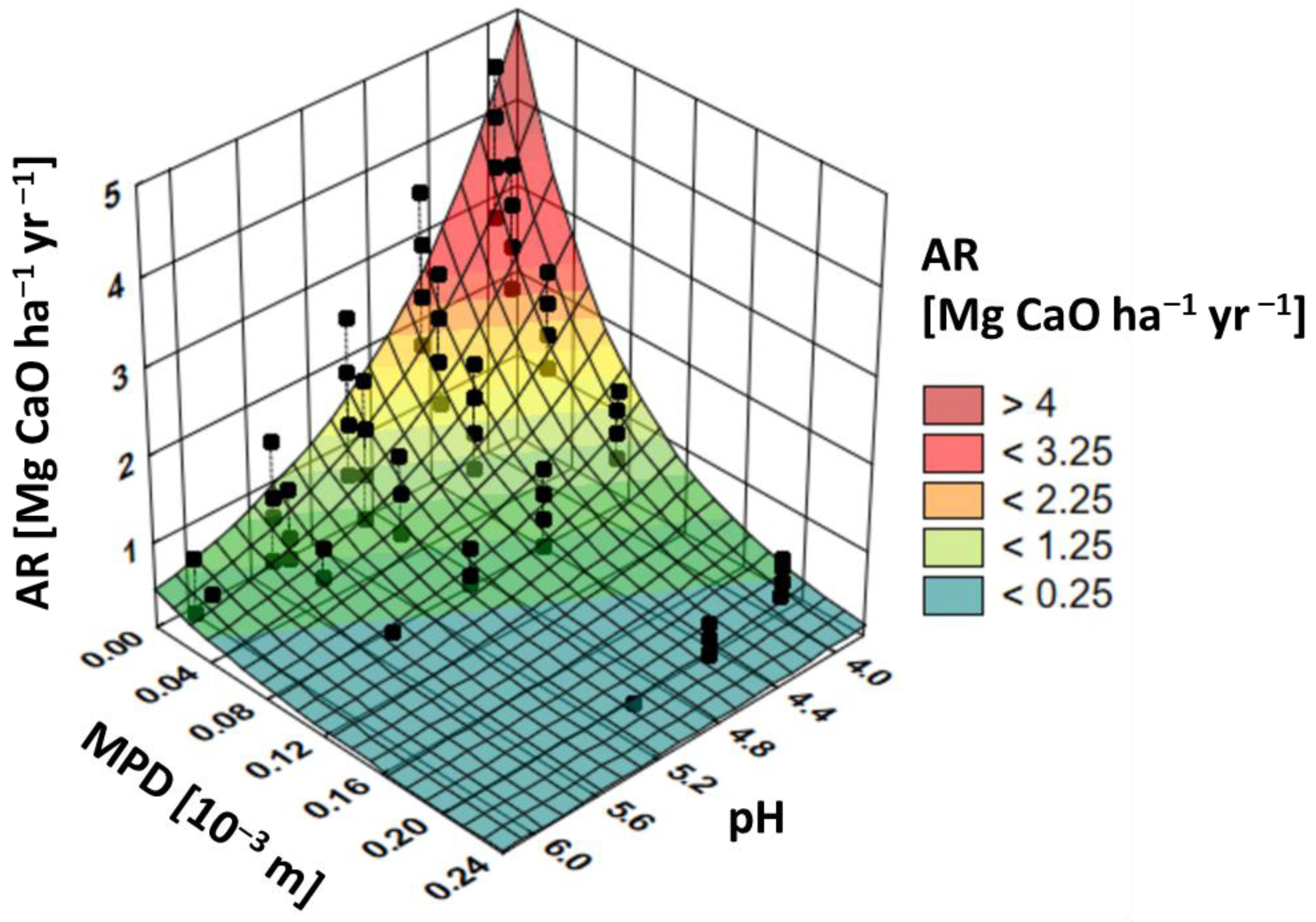
  • Decreases if the SOC increases because the buffer capacity is linearly related to the SOC [36];
  • Increases if the MPD increases because the buffer capacity is linearly related to the clay content [18] (which is inversely related to the MPD).
To parameterize the BNC approach, we applied Equation (3) to the calibration dataset. The predicted values of the three dimensionless fitting parameters are α = 0.685 (0.017), β = 2.642 (0.211) and γ = 0.054 (0.004), with the standard errors in parentheses. The regression between the measured and predicted Δ p H has R2 = 0.781 and RMSE = 0.19. Thereafter, we applied the parameterized BNC approach to the validation dataset, resulting in R2 = 0.778 and RMSE = 0.25. The results of both the model calibration and validation are separately visualized for the three test sites (Figure 2).
The application of different Ca(OH)2 concentrations led to pH changes between 0.1 and 7.6 pH units. For the calibration, the mathematical model (Equation (3)) was able to explain approximately 94% of the variability in the pH changes after Ca(OH)2 addition. Also, the slopes of the regression functions for the predicted vs. observed pH changes (Figure 1) were close to 1. The intercepts were close to zero, which implies that the systematic errors in shift and scale are negligible. When the model was applied to the validation data set, the model performance indices are in the same range. From these results, it can be concluded that the variables pH0, MPD and SOC are the main predictors of pH changes after Ca(OH)2 addition. Considering that we used soils of different origin (compare Section 2.1), the effects of different geological substrates and the resulting differences in the mineral-specific buffer capacities [37,38] seem to be less effective within the mentioned soil selection compared to the three factors included in the BNC approach. The test dataset described in Section 2.4 was used to compare the outputs of both the VDLUFA and the BNC approaches. The total test dataset was first used to calculate the CaO amounts necessary to change the given pH0 values to the pHtarget as calculated using the VDLUFA approach. Second, we excluded 70 data points from further calculations, where these calculated CaO amounts were negative because pH0 > pHtarget. Then, we applied the BNC approach to the remaining 90 data points to calculate the C a O H 2   amount necessary to obtain the same pH changes as calculated using the VDLUFA approach.
As mentioned in the introduction section, the LR for farmers, e.g., the VDLUFA approach, considers both the lime amount required to change the pH0 to pHtarget (Task A) and the lime amount that is necessary to compensate for the pH changes during one liming interval, e.g., 3 years (Task B). Consequently, the liming recommendation according to the VDLUFA should generally show higher CaO demands for the abovementioned pH change. In Figure 3, the results of applying both the BNC and the VDLUFA approaches to the created test dataset are shown separately for the four SOC levels. The required CaO amounts calculated using the BNC approach (CaOBNC) increases when the SOC also increases. This is because the soil’s buffer capacity is linearly related to the SOC [36]. The CaO amounts calculated using the VDLUFA approach (CaOVDLUFA) showed an inverse behavior as exemplified for a clayey soil (MPD = 0.005) and a loamy (MPD = 0.017) soil. This happens because the SOM counteracts Al toxicity by forming complexes with the Al ions [39,40]. This results in lower VDLUFA pHtarget values and accordingly lower recommended lime amounts.
The slopes of the regression functions presented in the caption of Figure 3 show that CaOBNC has an increase of approximately one-sixth that of the CaOVDLUFA. This is lower than the required lime amount estimated by Vogel et al. [13], who predicted a corresponding slope of 1/10 by applying the class-based VDLUFA look-up table values. However, their dataset had a lower CaOVDLUFA recommendation range with a maximum of approximately 5 mg ha−1.
The reader should bear in mind that the VDLUFA approach considers both the amount of lime required to change the pH0 to the pHtarget and the amount of lime that is necessary to compensate for the pH changes during one liming interval. However, the BNC approach solely considers the amount of lime needed to raise the pH from the pH0 to the pHtarget. The numerical difference between both approaches yields the acidification rate during the liming interval. In Figure 4, the annual AR, considering 3 years per liming interval, is shown as being dependent on the MPD and pH0.
The AR was predicted using the following model (Equation (4)):
A R = a × e x p ( b × p H 0 ) × e x p ( c × M P D )
with a = 226.82 (90.96), b = 1.008 (0.093) and c = 15.14 (1.92).
Generally, the calculated AR is related to the applied CaO amount as recommended by the VDLUFA, which increases when the MPD and pH0 decrease. Relatively low AR values < 0.25 Mg ha−1 were estimated for a broad range of MPD-pH0 combinations but mainly for sandy soils (MPD > 0.042 × 10⁻³ m) (compare Section 2.4). However, excessive AR values up to approximately 4 Mg CaO ha−1 yr−1 were predicted for loamy and clayey soils (MPD < 0.042 × 10⁻³ m) in combination with lower pH0 values. These values clearly exceed the maximum AR of approximately 0.85 Mg CaO ha−1 yr−1 [1,19,20,21,22].
Since up to four AR values per MPD–pH0 combination are related to different SOC values, as explained in the caption of Figure 3 and in Section 2.4, we extended Equation (4) via an SOC term (Equation (5)).
A R = a × e x p b × p H 0 × e x p c × M P D d × S O C
where a = 83.46 (14.18), b = 0.736 (0.040), c = 8.33 (0.61) and d = 0.036 (0.003).
Including the SOC term improves the model performance from R2 = 0.722 (Equation (4)) to R2 = 0.918 while reducing the RMSE from 0.502 Mg CaO ha−1 yr−1 to 0.308 Mg CaO ha−1 yr−1 (Equation (5)) (Figure 5).
Finally, we want to focus on Ca leaching as a relevant lime loss process considered in several lime loss regression models [1,21]. The global relationship between water balance and the soil pH was evaluated by Slessarev et al. [25]. They observed an abrupt transition from an alkaline to acidic soil pH that occurs at the point where the mean annual precipitation begins to exceed the mean annual potential evapotranspiration. The VDLUFA look-up tables were developed based on field experiments in the eastern part of Germany [15] in regions with a mean annual climatic water balance (precipitation–potential evapotranspiration) of −100 to 100 mm [41]. However, the VDLUFA look-up tables are more or less uniformly applied in Germany, neglecting that the climatic water balance ranges between −250 and 1200 mm yr−1 as estimated at 40 selected climate stations [42]. Consequently, using the climatic water balance as a site-dependent factor might further improve the efficiency of liming and allow for it to be adapted to a changing climate.

4. Conclusions

A new pedotransfer function for quantifying the liming-induced pH changes dependent on the pH0, MPD and SOC was established. For future research, we strongly recommend testing and recalibrating the BNC approach (Equation (3)) on the data of soils with a larger variety, especially in the geological parent material.
Comparing the outputs of both the VDLUFA and the BNC approaches enabled an estimation of the annual acidification rate as being dependent on the pH0, soil texture and SOC for site conditions in eastern Germany. The predicted above-average acidification rate values of up to approximately 4 Mg CaO ha−1 yr−1 raise questions for the main acidification process responsible. Since the acidification process depends on the climate conditions, management practices and other factors, the acidification rate varies in space and time. Therefore, we suggest a decoupling of the lime rate calculation, i.e., to separately calculate the amount of lime required to change the pH from the pH0 to the pHtarget and the amount of lime that is necessary to compensate for acidification. This might be helpful to optimize LRs adapted to different regions, varying management strategies and a changing climate.

Author Contributions

Conceptualization, J.R., S.V., R.G. and E.K.; methodology, J.R. and S.V.; validation, J.R.; investigation, J.R., S.V., R.G., E.B., C.K., K.L., A.N., G.P. and I.S.; data generation, S.V., E.B., F.G., C.K., K.L., A.N., G.P., S.P., D.S. and I.S.; writing—original draft preparation, J.R.; writing—review and editing, J.R., S.V., E.K., E.B., S.M., R.G. and I.S.; visualization, J.R. and E.B.; supervision, E.K., R.G. and J.R.; project administration, E.K.; funding acquisition, E.K., R.G. and J.R. All authors have read and agreed to the published version of the manuscript.

Funding

This work was conducted within the project ‘pH-BB: precision liming in Brandenburg’ (http://phbb.com (accessed on 30 August 2023)), which is part of the agricultural European Innovation Partnership program (EIP-AGRI) to improve agricultural productivity and sustainability (project no. 204016000014/80168341). The program is funded by the European Agricultural Fund for Rural Development of the European Commission and by the Ministry of Rural Development, Environment and Agriculture of the state of Brandenburg in Germany. Additional support was received from the German Ministry of Education and Research (BMBF) within the project I4S—Integrated System for Site-Specific Soil Fertility Management (grant no. 031B50513A).

Acknowledgments

The authors want to thank the three anonymous reviewers for their suggestions and helpful comments regarding the manuscript.

Conflicts of Interest

The authors declare no conflict of interest. The funders had no role in the design of the study; in the collection, analyses, or interpretation of data; in the writing of the manuscript, or in the decision to publish the results.

References

  1. Chambers, B.J.; Garwood, T.W.D. Lime loss rates from arable and grassland soils. J. Agricult. Sci. 1998, 131, 455–464. [Google Scholar] [CrossRef]
  2. von Wulfen, U.; Roschke, M.; Kape, H.-E. Guide Values for the Investigation and Advice as well as for the Technical Implementation of the Fertilizer Ordinance (DüV): Common Information from the States of Brandenburg, Mecklenburg-Western Pomerania and Saxony-Anhalt, Güterfelde, Germany; Landesamt für Verbraucherschutz & Landwirtschaft und Flurneuordnung (LVLF): Güterfelde, Germany, 2008. (In German) [Google Scholar]
  3. de Haan, J.J.; van Geel, W.C.A.; van Asperen, P.; Postma, R.; Brinks, H.; Reijneveld, A.; Malda, J.T. Handboek Bodem en Bemesting. Web Publication/Site, WUR. 2014. Available online: http://www.handboekbodemenbemesting.nl (accessed on 24 August 2023).
  4. Sinclair, A.; Crooks, B.; Coull, M. Soils Information, Texture and Liming Recommendations. In Technical Note TN656; SRUC. Scotland’s Rural College: Aberdeen, UK, 2014; Available online: https://www.google.com/url?sa=t&rct=j&q=&esrc=s&source=web&cd=&ved=2ahUKEwiCyreV6aKCAxXzh_0HHf0CChAQFnoECA0QAQ&url=https%3A%2F%2Fwww.sruc.ac.uk%2Fmedia%2F3acbc3rs%2Ftn656.pdf&usg=AOvVaw3eoj4iMfCYBWLvirPUmrvY&opi=89978449 (accessed on 24 August 2023).
  5. Söderström, M.; Sohlenius, G.; Rodhe, L.; Piikki, K. Adaptation of regional digital soil mapping for precision agriculture. Precis. Agric. 2016, 17, 588–607. [Google Scholar] [CrossRef]
  6. AHDB. Soil pH and Liming Recommendations for Arable and Grass Systems. Nutrient Management Guideline (RB209). Agriculture and Horticulture Development Board 2023, Coventry, UK. Available online: https://ahdb.org.uk/knowledge-library/soil-ph-and-liming-recommendations-for-arable-and-grass-systems (accessed on 30 August 2023).
  7. Tzilivakis, J.; Lewis, K.; Green, A.; Warner, D. ALA Lime Calculator [Software]; Agricultural Lime Association (ALA): London, UK, 2002. [Google Scholar]
  8. Vossen, P. Changing pH in Soil; University of California Cooperative Extension: Davis, CA, USA, 2002. [Google Scholar]
  9. Jacobs, A.; Flessa, H.; Don, A.; Heidkamp, A.; Prietz, R.; Dechow, R.; Gensior, A.; Poeplau, C.; Riggers, C.; Schneider, F.; et al. Arable Soils in Germany—Results of the Soil Status Survey; Johann Heinrich von Thünen-Institut: Braunschweig, Germany, 2018; 321p, Thünen Rep 64. (In German) [Google Scholar] [CrossRef]
  10. Bönecke, E.; Meyer, S.; Vogel, S.; Schröter, I.; Gebbers, R.; Kling, C.; Kramer, E.; Lück, K.; Nagel, A.; Philipp, G.; et al. Guidelines for precise lime management based on high-resolution soil pH, texture and SOM maps generated from proximal soil sensing data. Precis. Agric. 2020, 22, 493–523. [Google Scholar] [CrossRef]
  11. Meyer, S.; Kling, C.; Vogel, S.; Schröter, I.; Nagel, A.; Kramer, E.; Gebbers, R.; Philipp, G.; Lück, K.; Gerlach, F. Creating soil texture maps for precision liming using electrical resistivity and gamma ray mapping. In Precision Agriculture’19, Wageningen; Academic Publishers: Wageningen, The Netherlands, 2019; p. 92. [Google Scholar] [CrossRef]
  12. Ruehlmann, J.; Bönecke, E.; Meyer, S. Predicting the Lime Demand of Arable Soils from pH Value, Soil Texture and Soil Organic Matter Content. Agronomy 2021, 11, 785. [Google Scholar] [CrossRef]
  13. Vogel, S.; Bönecke, E.; Kling, C.; Kramer, E.; Lück, K.; Nagel, A.; Philipp, G.; Rühlmann, J.; Schröter, I.; Gebbers, R. Base Neutralizing Capacity of Agricultural Soils in a Quaternary Landscape of North-East Germany and Its Relationship to Best Management Practices in Lime Requirement Determination. Agronomy 2020, 10, 877. [Google Scholar] [CrossRef]
  14. Vogel, S.; Bönecke, E.; Kling, C.; Kramer, E.; Lück, K.; Philipp, G.; Rühlmann, J.; Schröter, I.; Gebbers, R. Direct prediction of site-specific lime requirement of arable fields using the base neutralizing capacity and a multi-sensor platform for on-the-go soil mapping. Precis. Agric. 2022, 23, 127–149. [Google Scholar] [CrossRef]
  15. Kerschberger, M.; Deller, B.; Hege, U.; Heyn, J.; Kape, H.E.; Krause, O.; Pollehn, J.; Rex, M.J.; Severin, K. Determination of the Lime Requirement of Arable and Grassland Soils; VDLUFA-Verlag: Darmstadt, Germany, 2000. (In German) [Google Scholar]
  16. Kerschberger, M.; Marks, G. Setting and maintaining a site-specific optimum pH value in the soil-a basic requirement for effective and environmentally compatible plant production. Berichte über Landwirtsch. 2007, 85, 56–77. (In German) [Google Scholar]
  17. Goulding, K.W. Soil acidification and the importance of liming agricultural soils with particular reference to the United Kingdom. Soil Use Manag. 2016, 32, 390–399. [Google Scholar] [CrossRef]
  18. Wang, X.; Tang, C.; Mahony, S.; Baldock, J.A.; Butterly, C.R. Factors affecting the measurement of soil pH buffer capacity: Approaches to optimize the methods. Eur. J. Soil Sci. 2015, 66, 53–64. [Google Scholar] [CrossRef]
  19. Bolton, J. Changes in magnesium and calcium in soils of the Broadbalk wheat experiment at Rothamsted from 1865 to 1966. J. Agric. Sci. 1972, 79, 217–223. [Google Scholar] [CrossRef]
  20. Bolton, J. Changes in soil pH and exchangeable calcium in two liming experiments on contrasting soils over 12 years. J. Agric. Sci. 1977, 89, 81–86. [Google Scholar] [CrossRef]
  21. Breemen, N.V.; Protz, R. Rates of calcium carbonate removal from soils. Can. J. Soil Sci. 1988, 68, 449–454. [Google Scholar] [CrossRef]
  22. Loide, V. About the effect of the contents and ratios of soil’s available calcium, potassium and magnesium in liming of acid soils. Agron. Res. 2004, 2, 71–82. [Google Scholar]
  23. BAD. Nutrient Losses from Agricultural Farms Managed According Good Agricultural Praxis; Bundesarbeitskreis Düngung: Frankfurt am Main, Germany, 2003. (In German) [Google Scholar]
  24. Archer, J. Crop Nutrition and Fertiliser Use; Farming Press Ltd.: Ipswich, MA, USA, 1985; p. 285. [Google Scholar]
  25. Slessarev, E.W.; Lin, Y.; Bingham, N.L.; Johnson, J.E.; Dai, Y.; Schimel, J.P.; Chadwick, O.A. Water balance creates a threshold in soil pH at the global scale. Nature 2016, 540, 567–569. [Google Scholar] [CrossRef]
  26. Brandenburg State Office for Mining, Geology and Raw Materials. Geological Map of the State of Brandenburg, Scale: 1:25,000 (GK 25). Cottbus, Brandenburg. Available online: https://geo.brandenburg.de/?page=Geologische-Karten&views=Ebenen----- (accessed on 1 August 2023).
  27. Shirazi, M.A.; Boersma, L.; Hart, J.W. A unifying quantitative analysis of soil texture: Improvement of precision and extension of scale. Soil Sci. Soc. Am. J. 1988, 52, 181–190. [Google Scholar] [CrossRef]
  28. DIN ISO 10694; Soil Quality—Determination of Organic and Total Carbon after Dry Combustion (Elementary Analysis). Beuth: Berlin, Germany, 1996.
  29. DIN ISO 11277; Soil Quality—Determination of Particle Size Distribution in Mineral Soil Material—Method by Sieving and Sedimentation. Beuth: Berlin, Germany, 2009.
  30. Sparks, D. Environmental Soil Chemistry, 2nd ed.; Academic Press, an Imprint of Elsevier: San Diego, CA, USA, 2003. [Google Scholar]
  31. Sposito, G. The Chemistry of Soils, 3rd ed.; Oxford University Press: New York, NY, USA, 2016. [Google Scholar]
  32. Meiwes, K.J.; Koenig, N.; Khana, P.K.; Prenzel, J.; Ulrich, B. Chemical test methods for mineral soils, litter layers and roots to characterize and evaluate acidification in forest soils. In Die Erfassung des Stoffkreislaufs in Waldökosystemen—Konzeption und Methodik. Berichte des Forschungszentrums Waldökosysteme/Waldsterben, Bd. 7; Meiwes, K.-J., Hauhs, M., Gerke, H., Asche, N., Matzner, E., Lammersdorf, N., Eds.; Institut für Bodenkunde und Waldernährung der Universität Göttingen: Göttingen, Germany, 1984. (In German) [Google Scholar]
  33. Kvalseth, T.O. Cautionary Note about R2. Am. Stat. 1985, 39, 279–285. [Google Scholar]
  34. Alexander, D.L.; Tropsha, A.; Winkler, D.A. Beware of R 2: Simple, unambiguous assessment of the prediction accuracy of QSAR and QSPR models. J. Chem. Inf. Model. 2015, 55, 1316–1322. [Google Scholar] [CrossRef]
  35. Curtin, D.; Trolove, S. Predicting pH buffering capacity of New Zealand soils from organic matter content and mineral characteristics. Soil Res. 2013, 51, 494–502. [Google Scholar] [CrossRef]
  36. Magdoff, F.R.; Bartlett, R.J. Soil pH buffering revisited. Soil Sci. Soc. Am. J. 1985, 49, 145–148. [Google Scholar] [CrossRef]
  37. Magdoff, F.R.; Bartlett, R.J.; Ross, D.S. Acidification and pH buffering of forest soils. Soil Sci. Soc. Am. J. 1987, 51, 1384–1386. [Google Scholar] [CrossRef]
  38. Schilling, G. Plant Nutrition and Fertilization; Verlag Eugen Ulmer: Stuttgart, Germany, 2000; p. 464. (In German) [Google Scholar]
  39. Bloom, P.R.; McBride, M.B.; Weaver, R.M. Aluminum organic matter in acid soils: Buffering and solution aluminum activity. Soil Sci. Soc. Am. J. 1979, 43, 488–493. [Google Scholar] [CrossRef]
  40. Büchner, M.; Gerstengarbe, F.-W.; Gottschalk, P.; Gutsch, M.; Hattermann, F.F.; Huang, S.; Koch, H.; Lasch, P.; Lüttger, A.; Schellnhuber, H.J.; et al. Climate Impact on Germany; Potsdam-Institut für Klimafolgenforschung: Potsdam, Germany, 2012. (In German) [Google Scholar]
  41. Henrichs, M.; Langner, J.; Uhl, M. Development of a simplified urban water balance model (WABILA). Water Sci. Technol. 2016, 73, 1785–1795. [Google Scholar] [CrossRef] [PubMed]
  42. Soil Science Division Staff. Soil Survey Manual; Ditzler, C., Scheffe, K., Monger, H.C., Eds.; USDA Handbook 18; Government Printing Office: Washington, DC, USA, 2017. Available online: https://www.nrcs.usda.gov/resources/guides-and-instructions/soil-survey-manual (accessed on 30 August 2023).
Figure 1. Clay, silt and sand contents (black dots) of the used soil samples as classified according to the German VDLUFA classification [16] (left) and the USDA system [26] (right).
Agronomy 13 02762 g001
Figure 2. Predicted pH changes after Ca(OH)2 addition vs. pH changes observed according to Equation (3) as applied to the calibration (top) and validation datasets (bottom) and as separately visualized for the three test sites.
Agronomy 13 02762 g002
Figure 3. Lime amounts required to change the pH from pH0 to pHtarget as calculated using the BNC (CaOBNC) and the VDLUFA (CaOVDLUFA) approaches (dots), respectively, and grouped based on SOC levels as mentioned in Section 2.4. The specifications of corresponding linear regression functions (lines) are given below. Within the gray shaded fields, two different mean particle diameter (MPD) groups with the same initial pH (pH0) value (see Section 2.4) are indicated. Linear regression lines are colored corresponding to the SOC level with following specifications: SOC = 5 g kg−1: y = 0.161x + 0.164, R2 = 0.320, RMSE = 0.225; SOC = 10 g kg−1: y = 0.162x + 0.414, R2 = 0.493, RMSE = 0.200; SOC = 20 g kg−1: y = 0.166x + 0.735, R2 = 0.942, RMSE = 0.183; SOC = 30 g kg−1: y = 0.161x + 1.2658, R2 = 0.798, RMSE = 0.141.
Agronomy 13 02762 g003
Figure 4. Annual acidification rate (AR) (Mg CaO ha−1 yr−1) dependent on mean particle diameter (MPD) and initial soil pH (pH0). Per MPD–pH0 combination, up to four AR values are shown, resulting from the four SOC contents of 5, 10, 20 and 30 (g kg−1), as mentioned in the created dataset (Section 2.4).
Agronomy 13 02762 g004
Figure 5. Acidification rates (ARs) estimated via the difference between the VDLUFA and the BNC approaches. ARobs vs. ARpred according to Equation (4) without SOC term (left) and according to Equation (5) with SOC term (right).
Agronomy 13 02762 g005
Table 1. Lime equivalents (kg CaO ha−1 yr−1) to compensate acidification due to neutralization and leaching as dependent on soil texture, land use and annual precipitation (after [23]).
Soil TextureLand UseLime Equivalents to Compensate Acidification
(kg CaO ha−1 yr−1)
Annual Precipitation
<600 mm600–750 mm>750 mm
sandyArable land300400500
Grass land150250350
loamyArable land400500600
Grass land200300400
clayeyArable land500600700
Grass land250350450
Table 2. MPD, SOC and initial pH values of the five test fields of the three farms.
Farm IFarm IIFarm III
MPD [10−3 m]
Min0.010.050.01
Max0.210.150.29
SD0.050.030.09
SOC (g kg−1)
Min4.406.405.75
Max32.3012.6026.2
SD5.111.256.66
Initial pH
Min5.245.714.51
Max7.557.327.24
SD0.490.340.77
Disclaimer/Publisher’s Note: The statements, opinions and data contained in all publications are solely those of the individual author(s) and contributor(s) and not of MDPI and/or the editor(s). MDPI and/or the editor(s) disclaim responsibility for any injury to people or property resulting from any ideas, methods, instructions or products referred to in the content.

