Abstract
Deep-learning-based methods for plant disease recognition pose challenges due to their high number of network parameters, extensive computational requirements, and overall complexity. To address this issue, we propose an improved residual-network-based multi-plant disease recognition method that combines the characteristics of plant diseases. Our approach introduces a lightweight technique called maximum grouping convolution to the ResNet18 model. We made three enhancements to adapt this method to the characteristics of plant diseases and ultimately reduced the convolution kernel requirements, resulting in the final model, Model_Lite. The experimental dataset comprises 20 types of plant diseases, including 13 selected from the publicly available Plant Village dataset and seven self-constructed images of apple leaves with complex backgrounds containing disease symptoms. The experimental results demonstrated that our improved network model, Model_Lite, contains only about 1/344th of the parameters and requires 1/35th of the computational effort compared to the original ResNet18 model, with a marginal decrease in the average accuracy of only 0.34%. Comparing Model_Lite with MobileNet, ShuffleNet, SqueezeNet, and GhostNet, our proposed Model_Lite model achieved a superior average recognition accuracy while maintaining a much smaller number of parameters and computational requirements than the above models. Thus, the Model_Lite model holds significant potential for widespread application in plant disease recognition and can serve as a valuable reference for future research on lightweight network model design.
1. Introduction
Plant diseases significantly impact growers’ productivity [1,2,3]. Weather, the environment, microorganisms, viruses, and bacteria make plants vulnerable to various diseases during their growth. Among these diseases, leaf diseases are the most commonly encountered. However, relying solely on visual observation and empirical judgment often proves challenging for the timely and accurate identification of disease types due to the large number of diseases and their similarities. Consequently, delayed diagnosis exacerbates disease spread and leads to significant losses in crop yield and economic benefits. Therefore, it is imperative to swiftly and accurately determine disease types to facilitate effective plant disease control.
Traditional plant disease recognition algorithms [4,5,6] have significantly progressed in extracting and analyzing image features using conventional classification methods. For instance, Wu et al. [7] extracted features, including color, HSV, texture, and histograms of directional gradients, from diseased grape leaf images. They employed principal component analysis (PCA) for dimensionality reduction and a multi-feature fusion approach for feature vector formation. Ultimately, the support vector machine (SVM) algorithm was utilized for disease recognition, achieving an accuracy of 92.5%. Mokhtar et al. [8] utilized a support vector machine (SVM) algorithm with different kernel functions for the classification and identification of tomato mosaic disease with an average accuracy of 92%. Despite the success of these approaches, the manual feature extraction process is intricate and subjective, making it difficult to determine an optimal and robust feature set. Furthermore, plant diseases often exhibit comprehensive features encompassing texture, shape, and color, posing significant challenges to traditional plant leaf disease recognition algorithms and limiting improvements in recognition outcomes.
The advent of deep learning has introduced a novel approach to disease recognition. Plant leaf disease recognition methods based on convolutional neural networks (CNNs) [9,10,11] offer notable advantages, including independence from specific features and high recognition accuracy. For instance, Yang et al. [12] proposed a fine-grained classification model, LFC-Net, with a self-supervised mechanism to classify images of eight tomato diseases and healthy leaf images with 99.7% accuracy. X Sun et al. proposed a transfer-learning-based method for maize disease recognition, fine-tuning pre-trained inception series network models, resulting in an improved recognition accuracy and reduced training time [13]. Yan et al. presented an enhanced model based on VGG16 for identifying apple leaf diseases, achieving an overall accuracy of 99.01% in apple leaf classification [14]. By replacing the first layer of the convolutional kernel with three 3 × 3 convolutional kernels and adjusting the base number to 64, Wang et al. achieved a recognition accuracy of 90.22% in detecting 276 actual corn disease images using an improved version of the original ResNeXt101 model [15]. However, traditional enhanced CNNs and similar approaches fail to further analyze disease features, exhibiting numerous parameters and high computational complexity. Although these methods yield superior recognition results, they necessitate abundant computational resources and extensive storage space for operation, thereby limiting their application in resource-constrained mobile devices. Consequently, there is a growing demand for lightweight network models that offer a high performance with a low computational cost in plant disease recognition applications in real-life scenarios. A typical neural-network-lightweighting approach replaces the original convolutional layers using depth-separable convolution. However, the introduced depth-separable convolution may ignore or lose some vital information, which leads to a decrease in the recognition accuracy of the model [16,17,18,19]. We also tried depth-separable convolution as a lightweighting strategy in our initial experiments, which resulted in about a 2% decrease in the recognition accuracy of the model without shrinking the convolution kernel.
So, based on depth-separable convolution, we propose a new lightweighting method. We removed the pointwise convolution operation in depth-separable convolution and set the number of groups to the number of input channels in the depthwise convolution operation, which we call extreme grouping convolution. Considering the advantages of ResNet18 [20], such as its small size, good performance, and extensibility with a modular design, we used it as our improved model.
Our improvement points are as follows:
- (1)
- We used the extreme grouping convolution method to replace the original model convolutional layer in order to reduce the number of model parameters and computation amount to achieve lightweighting while maintaining the recognition accuracy.
- (2)
- Considering the characteristics of extreme grouping convolution, there is less information interaction between groups. We added an SE [21] attention module with a squeeze ratio of 16 to each basic block, which promotes the information interaction between groups and, at the same time, emphasizes the critical diseases and suppresses the influence of irrelevant factors on the model.
- (3)
- Combining the characteristics of small and similar plant lesions, we canceled the downsampling in layers 3 and 4 of the model, increased the resolution of the feature map to 4 times that of the original, and introduced dilated convolution [22] to maintain the size of the receptive field of the model.
- (4)
- We improved the residual connection in the original model so that the model can learn the errors of two neighboring layers to further improve the performance of the network model.
- (5)
- Finally, by reducing the number of convolution kernels to (16, 32, 64, 128) and removing the network redundancy, we constructed a lightweight residual network called Model_Lite.
2. Materials and Methods
2.1. Dataset Construction
2.1.1. Acquisition of Datasets
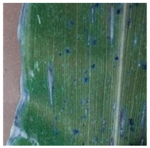
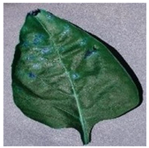
The dataset of this study contained two parts with a total of 18,491 plant disease images, aiming to better fit the actual plant disease recognition situation and enhance the robustness and generalization ability of the model. The first part of the set of disease images was taken at the experimental apple field of Jilin Agricultural University in Changchun, Jilin Province, and a small number of them were obtained online. The shooting was conducted from 8:00 a.m. to 5:00 p.m., and the images were taken with an iPhone 13 device with 3024 × 4032 pixels. After being recognized by agricultural experts, 6686 apple disease images in seven categories with complex backgrounds were finally obtained. Characterized by the fact that they were all taken under natural light conditions, the environments were complex and conformed to the actual situation, as shown in Figure 1n–t. The second part included simple background disease images, covering 13 categories and totaling 11,805 images, which were selected from the Plant Village [23] dataset and characterized by a standardized shooting and laboratory background environment, which was used as a complement to the first part of the data, as shown in Figure 1a–m.
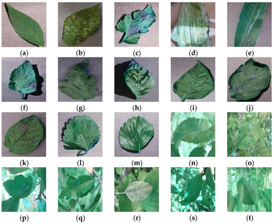
Figure 1.
Sample dataset. The sample (a–t) categories are explained in Table 1 below.
2.1.2. Data Preprocessing
Due to the existence of dataset images with different sizes, to reduce the recognition errors caused by image irregularities, the image size was first uniformly adjusted to 256 × 256 pixels, and then the training set and validation set were divided according to a ratio of 8:2. Before feeding the images into the model, central cropping was performed to resize them to 224 × 224 pixels while maintaining their width and height. Additionally, data standardization was applied to enhance the model’s stability and training efficiency. Table 1 displays the distribution of samples for different types of plant diseases in the dataset. In order to improve the diversity of the dataset and mitigate the risk of overfitting, several data augmentation techniques were employed. These techniques included randomly applying horizontal or vertical flips, random rotation, simulating rain and foggy weather, color dithering, and affine transformation. This augmentation process aimed to enhance the model’s generalization ability. Figure 2 provides examples of samples before and after data augmentation. Horizontal and vertical flips and random rotations simulated variations in the plant leaf morphology encountered in real-life scenarios. Simulating rainy and foggy weather was used to replicated detection situations during inclement weather. Brightness adjustment was used to capture the diverse lighting conditions associated with sunny and cloudy weather. Lastly, affine transformation allowed for the simulation of various shooting angles.

Table 1.
Number of samples for each disease in dataset.
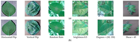
Figure 2.
(a) Original images; (b) Augmented images.
2.2. Experimental Design
2.2.1. Introduction to Group Convolution
Grouped convolution [24] was employed as a replacement for all the convolutional layers within the original ResNet18 model. This approach, based on the split–transform–merge concept [25], balances high recognition accuracy, a reduced number of parameters, and computational efficiency. By utilizing grouped convolution, feature maps with distinct focus points are obtained, which complement each other and provide a more comprehensive representation of the image features. Additionally, grouped convolution enhances the diagonal correlation among convolution kernels, reducing the number of parameters and alleviating overfitting issues, similar to regularization techniques.
The grouped convolutional computation process is shown in Figure 3 (c is the number of input feature map channels, c′ is the number of convolution kernels, g is the number of subgroups, k is the convolution kernel size, and W′ and H′ are the output feature map dimensions). Grouped convolution decomposes the input feature map and performs convolution operations on each grouping. Since the number of input and output channels for convolution is reduced, the parameters and computation are also reduced. The ratios of the number of parameters and the computation amount of the grouped convolution operation to the ordinary convolution operation are shown in the following equations (Equations (1) and (2)), which show that when the number of groupings is g, the number of parameters and the computation amount of the grouped convolution is 1/g of the ordinary convolution.
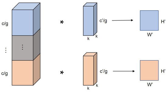
Figure 3.
Grouped convolutional operation process.
2.2.2. SE Attention Module Addition
To mitigate the influence of complex background classes and irrelevant factors in the plant disease images, this study incorporated the SE (squeeze-and-excitation networks) attention module. The SE module is a lightweight attention mechanism designed to enhance inter-channel attention, thereby improving the model’s ability to extract crucial disease features while reducing the impact of other interferences and enhancing the disease recognition performance. The structure of the SE module consists of two components: squeeze and excitation. Figure 4 illustrates the architecture of the SE module. The squeeze component utilizes global average pooling to capture contextual information for each channel dimension of the feature map. This process compresses the 2D features (H × W) of each channel into a single actual number, transforming the feature map [h, w, c] into [1, 1, c], thus obtaining global features at the channel level. In the excitation component, two fully connected layers generate weight values for each feature channel, establishing correlations among the channels. The output weights align with the number of input feature map channels, and the weights for the different channels are learned based on their relationships. These weights are then normalized and applied to the features of each channel through a scale operation. By incorporating the SE module, the model learns to assign higher weights to important features while reducing the sensitivity to irrelevant features. This mechanism allows the model to focus on disease-related characteristics, selectively enhancing the disease recognition performance.
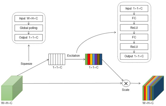
Figure 4.
SE module structure diagram.
2.2.3. Improved Feature Map Resolution
Considering that the nuances in plant diseases mainly stem from their differences, it has been observed that the original ResNet18 model experiences a reduction in the feature map resolution to 7 × 7 after four layers of downsampling. This decrease in the resolution leads to a significant loss of spatial information and hampers the model’s ability to extract features effectively. This study adopted a solution to address this limitation by eliminating the downsampling operations in layer 3 and layer 4 of the original model. Instead, dilated convolution with an expansion factor of 2 was incorporated to maintain an unchanged receptive field. By doing so, the resolution of the subsequent feature maps in layers 3 and 4 is kept at 28 × 28, thus preserving more spatial information about the plant disease. This modification successfully resolves the issue of low-resolution feature maps, which mitigates the problem of inadequate feature extraction in the model. The improved structure of the model, incorporating dilated convolution and maintaining higher-resolution feature maps, is illustrated in Figure 5.
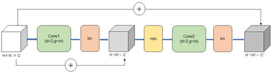
Figure 5.
Basic module structure diagram of layer 3 and layer 4.
2.2.4. Improved Residual Connection
By incorporating factors such as plant disease color, texture, and contour, it is evident that plant diseases exhibit certain similarities in their features, while different instances of the same plant disease pose challenges in terms of discrimination. To address this, residual learning is utilized, significantly enhancing the network’s ability to extract disease features. Consequently, residual networks have been widely adopted in plant disease recognition research [26,27,28]. A residual block can be expressed as shown in the following equation (Equation (3)) (XL and XL + 1 are the Lth and (L + 1)th layer feature maps, respectively, WL is the Lth layer convolution parameter, and F is the convolution operation parameter):
That is, by transforming the desired complex mapping H(XL, WL):=XL + 1 to H(XL, WL):=XL + F(XL, WL), the superimposed convolutional layers only need to fit F(XL, WL):=H(XL, WL) − XL. This transformation makes it easier to optimize the deeper network, assuming that the network learns XL optimally and that the convolution of the deeper layers of the network with the weights set to 0 will be able to remain in the later convolutional layers without causing accuracy degradation. If the optimal result approximates XL, the deeper convolutional layers will mostly only be fine-tuned rather than learning a new mapping. The residual structure is simple, as shown in Figure 6a below. The residual module improves the performance of the deeper network by introducing shortcut connections (cross-layer connections), which preserve the information in the previous layers in the training of the network and reduce the risk of gradient vanishing.
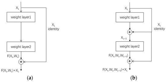
Figure 6.
(a) Regular residual connection; (b) improved residual connection.
On the other hand, the improved connection updates the learning parameters by learning the residuals of the two neighboring layers, which is based on the same principle as the original residual connection. Its computational formula can be expressed as the following equation (Equation (4)) (where XL and XL+1 denote the inputs of the Lth and (L + 1)th layers, respectively, F denotes the mapping function between the residual blocks of the two layers, and WL and WL+1 denote the weight matrices of the Lth and (L + 1)th layers, respectively):
The enhanced residual connection, as depicted in Figure 6b, is introduced. This improved design incorporates a two-layer residual connection, enabling the network to learn from the errors of adjacent network layers and the errors of the two neighboring layers. This advancement facilitates a more refined network update process and promotes comprehensive and intricate feature learning.
2.2.5. Convolution Kernel Reduction
By adjusting the number of convolutional kernels within the model, we can explore its complexity and expressive power. Increasing the number of convolutional kernels enhances the feature expressiveness and consequently improves the model’s performance. However, it also escalates the computational requirements, increases the number of parameters, and may lead to overfitting issues. Conversely, reducing the number of convolutional kernels may diminish the model’s perceptual ability and recognition accuracy. Nonetheless, it efficiently reduces the model complexity and computational costs. Reducing the number of convolutional kernels allows us to eliminate network model redundancy, decrease computational effort, and simplify the model structure with minimal compromise in terms of recognition accuracy. This ensures optimal model performance while achieving the objective of model lightweighting.
2.2.6. Lightweight Residual Network Structure
A schematic representation of the lightweight residual network can be seen in Figure 7. This model is built upon the architecture of ResNet18. To improve the model’s performance and reduce computational requirements, the original convolution layers are replaced with group convolutions, where the number of groups equals the number of channels. This modification enhances the model’s efficiency while reducing the number of parameters. In order to accentuate the disease characteristics and strengthen inter-group information interactions within the group convolution, an SE (squeeze-and-excitation) module is incorporated after each basic block. This module helps the network to focus on important disease-related features.
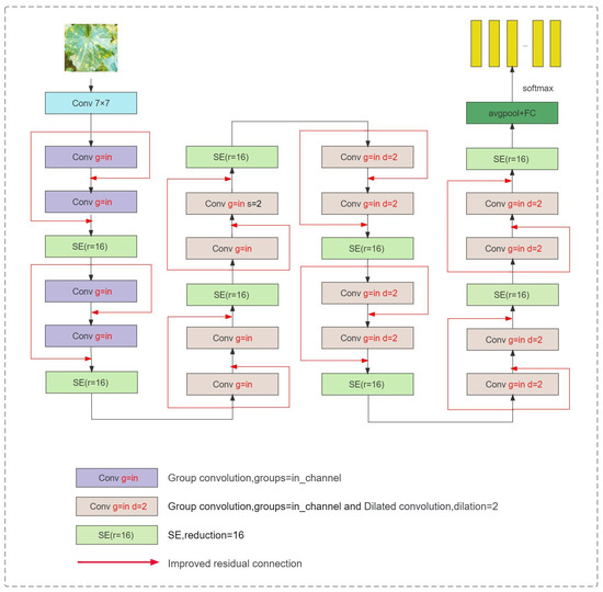
Figure 7.
Lightweight network structure diagram.
Furthermore, in layers 3 and 4, the downsampling operation in the initial convolutional layer of the traditional residual structure is removed. This adjustment preserves the feature map resolution at 28 × 28, allowing for more spatial feature information to be captured. To maintain an intact receptive field, dilated convolutions are introduced. Lastly, the original residual connection is further improved to enhance the model’s overall performance.
2.3. Experimental Environment Setting
The experimental environment configuration used in this study is outlined in Table 2. The training process was conducted over 200 epochs, with a sample input size of 256 × 256. The ReLU activation function was employed, and the Adam optimizer was utilized. The cross-entropy function was applied for optimization purposes, with an initial learning rate of 0.001. A detailed step-by-step methodology flow for training the plant disease recognition model is illustrated in Figure 8.
Table 2.
Experimental environment configuration.
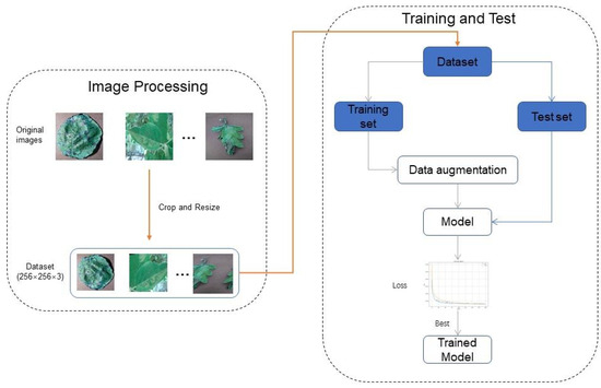
Figure 8.
Flowchart of the step-by-step methodology.
This study chose the average recognition accuracy, the number of network parameters, and the million floating point operations per second (MFLOPs) as the metrics for evaluating the network.
The average identification accuracy (P, %) refers to the ratio of correctly predicted samples to all observations in the model, as shown in Equation (5). In the equation, TPi and FPi denote the number of correctly and incorrectly predicted samples of disease samples of category I in the validation set, respectively, and N denotes the number of disease species. The average recognition accuracy measures the recognition accuracy of the model for the entire plant disease dataset of 20 diseases, which facilitates the comparison of the performance of different models from a macroscopic perspective.
The spatial complexity of an algorithm refers to the number of parameters in the model, which directly affects the hardware level and memory consumption. A smaller number of parameters indicates a smaller model capacity, which is beneficial for deployment on mobile devices with limited memory resources. On the other hand, the computation amount reflects the algorithm’s time complexity. It is crucial to minimize the computation amount while maintaining accuracy to improve the efficiency and processing speed of the model. The number of parameters and the computation amount are crucial indicators for evaluating the strengths and weaknesses of a network model. Therefore, it is essential to consider these two aspects when enhancing a network model comprehensively.
3. Results and Discussion
3.1. Experimental Analysis
3.1.1. Impact of the Number of Grouped Convolutions on the Model
To improve the original network and explore the effect of the number of groups on the network model, grouped convolution was added to each residual module of the original ResNet18 model in our study. We conducted experiments to construct three network models, namely Model_g16, Model_g32, and Model_gMax, where grouped convolutions were performed based on the original model. The groups used were 16, 32, and in_channel (the maximum number of groups equal to the number of input channels of the convolution layer), respectively. The corresponding loss curves are depicted in Figure 9, which illustrates the trends of the loss functions for the three different numbers of groups, i.e., 16, 32, and in_channel. As shown in Figure 9, the model exhibited rapid convergence and effectively captured the disease features. After five rounds of training, the recognition accuracy rate of the model exceeded 80%, and this rate was further improved to over 90% after sixteen rounds of training. This was because the model inherits the residual network’s excellent structure, making the network easier to optimize. The grouped convolution used can focus on different feature maps that complement each other to represent the image features more completely and improve the ability of the network model to fit the disease features. It is worth noting that there was a certain degree of overfitting in the model with only grouped convolution. The overfitting problem of the model was solved after adding subsequent improvement points, and the loss curve of the final lightweight model, Model_Lite, is shown in the following section (Section 3.4).
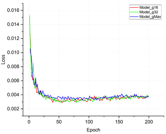
Figure 9.
Training loss curve plot.
The experimental results are summarized in Table 3. In Model_g16, where the grouping number was set to 16, the parameters were approximately 1/12 of the original model, while the computational operations decreased to about 1/7. Similarly, in Model_gMax with a maximum grouping number (equal to the number of input channels), the parameters were roughly 1/46 of the original model, and the computational operations decreased by around 1/11. The accuracy rate of Model_g16 exceeded that of the original model by 1.2%. This improvement can be attributed to two factors: first, with a grouping number of 16, there were more channels within each group, which enabled a better retention of the relevance among the input features and facilitated the transfer and integration of information, ultimately enhancing the model’s performance. Second, reducing the number of parameters and computational operations in Model_g16 helped to improve the overall efficiency. Model_g32 and Model_gMax exhibited accuracy improvements of 0.96% and 0.47%, respectively, compared to the average accuracy of the original model. Although these improvements were slightly lower than in Model_g16 with a grouping number of 16, the corresponding reduction in parameters and computational operations was more significant than in Model_g16.
Table 3.
Experiment results of group convolution.
We found that grouped convolution could also improve the model performance while significantly reducing the parameters and computation of the network model. The larger the number of groups, the smaller the number of parameters and analyses, but the recognition accuracy of the model was slightly reduced compared to the small number of groups.
3.1.2. Impact of the SE Attention Module on the Model
Based on Model_g16, Model_g32, and Model_gMax, we introduced the SE attention module between the BasicBlock models to explore the effect of the SE attention module on the performance of the network model.
Table 4 shows that the number of parameters and the computation volume of Model_g16, Model_g32, and Model_gMax increased slightly after adding the SE attention module. The average accuracies of Model_g32 and Model_gMax were improved by 0.06% and 0.48%, respectively. However, the average accuracy of Model_g16 was decreased by 0.37%. We know that the larger the number of groups, the less information interaction there is between groups. At the same time, the added SE module increased the information interaction between the different groups, especially for the model where the number of groups was equal to the number of channels, which improved the perceptual ability most obviously. In this experiment, the SE attention module was suitable for the models with a large number of groups and could improve the model accuracy at a small cost of computation and parameters. On the other hand, the average accuracy of Model_g16 decreased, probably because the model size and computational effort were already significant, and the addition of the SE module led to model redundancy and some overfitting phenomena.
Table 4.
Experiment results of the SE attention module.
3.1.3. Impact of Increased Feature Map Resolution on the Model
Based on the experiments above, we conducted further investigations by increasing the resolution of the feature map to 28 × 28 after eliminating downsampling in layer 3 and layer 4 of the network model. We replaced the original convolution with dilated convolution to preserve the receptive field. The objective was to examine the impact of the enhanced feature map resolution on the overall performance of the network model.
After removing the downsampling operation and introducing an increased feature map resolution through dilated convolution, there was no change in the number of model parameters. However, there was a significant increase in the computational requirements. Additionally, the model exhibited a minor degree of overfitting, resulting in a slight decrease in the average accuracy of Model_g16. Conversely, Model_g32 and Model_gMax improved the average accuracy by 0.26% and 0.53%, respectively. We know that different plant diseases are often manifested in subtle color and texture differences, and the downsampling operation will continuously reduce the image accuracy, which may lead to subtle but essential image features being overlooked in the process. Table 5 further reveals that, with the enhancement of the feature map resolution and the incorporation of dilated convolution, there was a slight decrease in the average accuracy of Model_g16 accompanied by a corresponding increase in the computation by 581.72 MFLOPs. On the other hand, Model_gMax achieved a maximum improvement in accuracy of 0.53% with a minimum increase in the computation of 145.49 MFLOPs. These results indicate that enhancing the feature map resolution and introducing dilated convolution in this experiment could be applied to the models with many grouped convolutional groups.
Table 5.
Experiment results of improving feature map resolution.
The comprehensive evaluation of the average accuracy, number of parameters, and computational volume revealed that the optimal model performance was achieved by incorporating the SE module and improving the resolution of the feature map simultaneously. Model_gMax exhibited the most remarkable improvement regarding the average accuracy, increasing by up to 0.87%. The elimination of downsampling and the subsequent increase in the feature map resolution ensured that the network did not overlook any critical fine-grained features associated with plant diseases. Furthermore, adding the SE module enhanced the network’s focus on crucial feature channels, promoting information interaction among the groups during group convolutions. These two components worked synergistically to enhance the overall network performance. For the subsequent experiments, the models with the SE module, increased feature map resolution, and dilated convolution were denoted as Model_16, Model_32, and Model_Max, respectively. This selection ensured consistency across Model_g16, Model_g32, and Model_gMax.
3.1.4. Impact of Improving Residual Connections on Model Performance
The original ResNet18 architecture updates the learning parameters by learning the network layer residuals of adjacent layers. However, as different plant disease features exhibit some similarities, enhancing the original one-layer residual connections to include two adjacent layers enhances the feature diversity and results in more refined network updates. This improvement leads to an enhanced feature extraction capability and generalization ability of the network. Table 6 presents the results of improving the residual connections (IRC) for Model_16, Model_32, and Model_Max. The number of parameters and the computational volume remained unchanged before and after the improvement since the calculation involved a simple matrix addition without requiring additional parameters to learn the connection. Among the models, Model_Max demonstrated a tremendous improvement in terms of the average accuracy, increasing by up to 0.19%. These findings prove that improving the residual connections could effectively enhance the model accuracy while maintaining the stability of the model parameters and computational effort.
Table 6.
Experimental results of improved residual connection.
3.1.5. Impact of Reducing the Number of Convolutional Kernels on Model Performance
To obtain the final lightweight model, this study conducted experiments on the Model_16, Model_32, and Model_Max models, which underwent an improvement in terms of residual connections. The objective was to reduce the number of convolution kernels used in the models. Specifically, the convolution kernels in the four layers were reduced to (32, 64, 128, 256) and (16, 32, 64, 128). The results of these experiments are presented in Table 7. It is important to note that for the Model_32 residual module, which had 32 subgroups for convolution, the condition did not hold when the number of convolution kernels was smaller than the number of subgroups.
Table 7.
Experimental results of reducing the number of convolution kernels.
From Table 7, it can be seen that when the number of convolutional kernels was (16, 32, 64, 128), Model_Max was comparable to the original ResNet18 model, with 1/344 of its number of parameters and 1/35 of its computation. At the same time, the average accuracy was decreased by only 0.34%. Model_16 had 1/167 of its number of parameters and 1/23 of its computation, while the average accuracy was decreased by 0.24%. When the number of convolutional kernels was (32, 64, 128, 256), Model_Max was comparable to the original ResNet18, with 1/113 of the number of parameters and 1/15 of the computation. The average accuracy was 0.78% higher than that of the original model. Model_32 had 1/65 of the number of parameters and 1/10 of the computation, and the average accuracy was 0.60% higher than that of the original model. Model_16 had 1/44 of the number of parameters and 1/163 of the computation, while the average accuracy was decreased by 0.24%. The number of parameters for Model_16 was 1/44, the calculation amount was 1/8, and the average accuracy was 0.42% higher than that of the original model.
From the above experimental results, we can see that when the number of convolutional kernels in the model is certain, the larger the grouping number of the model, the smaller the number of parameters and computation amount and the higher the average recognition accuracy of the model; When the number of convolutional kernels in the model decreases, the average recognition accuracy of the model will be slightly decreased, but it will still be maintained at a high level. However, the number of parameters and the model’s computation will be reduced significantly. This shows that increasing the convolutional kernels to improve the model recognition accuracy is costly and leads to a certain degree of redundancy in the model. By appropriately reducing the number of convolutional kernels, the model can be significantly streamlined with a slight reduction in the model’s recognition accuracy in order to achieve the purpose of model lightweighting. Finally, the Model_gMax model with its reduced number of convolutional kernels (16, 32, 64, 128) was selected as the final lightweight model, Model_Lite, by combining the average accuracy, the number of parameters, and the computation amount.
3.2. Comparison of Different Attention Mechanisms
To investigate the impact of different attention mechanisms on the performance of Model_Lite, three attention mechanisms were selected for comparison: the Self Attention spatial attention mechanism [29], the ECA channel attention mechanism (Efficient Channel and Attention) [30], and the CBAM channel spatial hybrid attention mechanism (Convolutional Block and Attention Module) [31]. These were compared to the SE channel attention mechanism used in the original model. The experimental results are presented in Table 8 below.
Table 8.
Experimental results of different attention mechanisms.
From Table 8, it can be observed that the SE and ECA channel attention mechanisms achieved optimal performance with a high model recognition accuracy while having low numbers of parameters and low computation amounts. The CBAM spatial channel mixing and attention mechanism was second only to the channel attention mechanism. In contrast, the Self Attention spatial attention mechanism had the lowest recognition accuracy and the most extensive computation amount and number of parameters. The reason for this is that channel attention applies weights to the feature map of each channel to represent its association with crucial information. As the feature map size tends to decrease with the increase in the number of dimensions in neural networks, channels represent the feature information of the entire image. Therefore, the channel attention mechanism can indicate important channel information for the model to effectively improve the network’s performance.
In contrast, spatial attention is applied to the spatial feature map, and the feature map used in the model was the only spatial feature map available. As the resolution of the feature map in a model decreases with the increase in the number of dimensions, spatial attention cannot provide a better enhancement effect. Therefore, the channel attention mechanism was better suited for the model in this scenario.
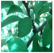
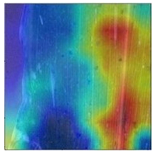
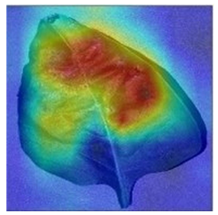
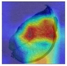
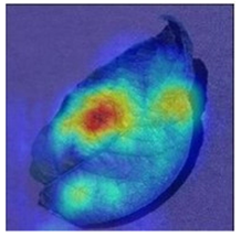
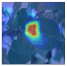
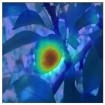
3.3. Visualization of Model Concerns
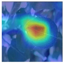
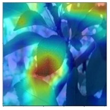
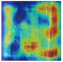
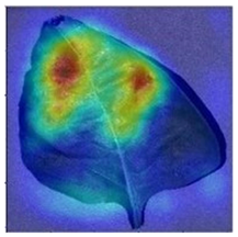
To better evaluate the improved model proposed in this experiment in terms of its ability to learn plant disease features, Grad-CAM [32] was employed to visualize the classification results. This study’s selected data samples from the test set were visualized using the Model_Lite model and the original ResNet18 network model. The last layer of the network was utilized for feature visualization. Table 9 shows that the Model_Lite model with its residual connection had a more accurate and comprehensive range of focus in terms of the heat map attention in the simple background types of diseases such as d, h, and k. The heat map attention of Model_Lite with the SE module in terms of the complex background of apple leaves was completely in the leaves, which thus avoided interference. These improvements in the focus of the heat map coincided with the functions of the added modules, indicating that the above modifications were helpful to the model’s performance.
Table 9.
Comparison of Grad-CAM heat maps.
3.4. Comparative Lightweight Network Experiments
To better evaluate the performance of the network, mainstream lightweight network models were selected in order to compare them with the final lightweight model, Model_Lite, and these control network models were the MobileNet [33], ShuffleNet [34], SqueezeNet [35], and GhostNet [36] series of lightweight network models.
The accuracy and loss curves for each network model are shown in Figure 10, from which it can be seen that Model_Lite’s curve convergence in the previous 20 rounds was significantly faster than that of other network models. The curves converged based on a higher level of accuracy thanks to the lightweight residual module and the final convolutional pruning operation, which reasonably removed redundant parameters from the model in order to reduce the complexity of the model and the model inference time, which in turn helped the model to converge more quickly.
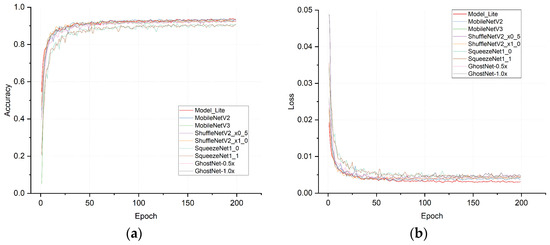
Figure 10.
(a) Accuracy curve plots; (b) loss curve plots.
The experimental results, as presented in Table 10, indicated that Model_Lite achieved the optimal performance based on the analysis of the average recognition accuracy. It surpassed the series of lightweight networks discussed earlier. Furthermore, Model_Lite exhibited a significantly smaller number of parameters than the other lightweight network models listed in the table. Additionally, the computational requirements were only slightly more prominent when compared to ShuffleNetV2_x0_5 [37] and Ghostnet-0.5x. Model_Lite’s outstanding performance can be attributed to its utilization of the excellent network structure inherited from ResNet18. Moreover, reasonable enhancements specific to the disease characteristics were incorporated. Lastly, by reducing the number of convolutional kernels in the model, the redundancy was effectively eliminated, resulting in a compact model size that maintained a high recognition accuracy.
Table 10.
Experimental results of lightweight network comparison.
3.5. Comparison of the Accuracy of Complex Background Disease Classification
To further investigate the performance of the models on the dataset, the confusion matrix for each lightweight model was obtained. Interestingly, it was observed that there was minimal variation in terms of the recognition accuracy among the models when classifying simple background images in the dataset. As a result, the primary discrepancy in the average recognition accuracy stemmed from the model’s ability to identify disease images with miscellaneous backgrounds. Figure 11 illustrates the confusion matrix specifically for Model_Lite on the validation set.
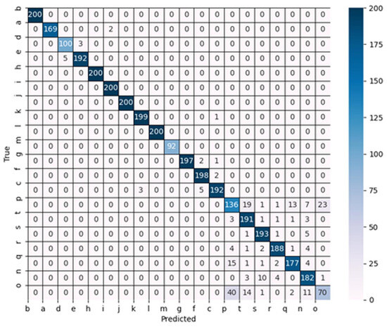
Figure 11.
Confusion matrix of Model_Lite.
As depicted in Figure 11, Model_Lite exhibited a noticeable increase in terms of the error when classifying diseases with complex backgrounds. However, it still demonstrated a significant improvement compared to the aforementioned lightweight network models. For further details, Table 11 presents the precision values for both Model_Lite and the selected lightweight network models when identifying disease species with complex backgrounds.
Table 11.
Accuracy of partial model identification of complex background diseases.
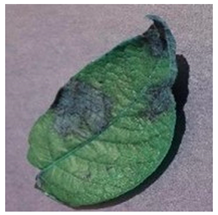
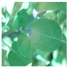
According to the results shown in Table 11, it can be seen that in terms of the recognition of disease species in images with complex backgrounds (p–o), Model_Lite achieved the highest recognition accuracy in all the four disease categories compared to the other network structures, and its sample images are shown in Figure 12.
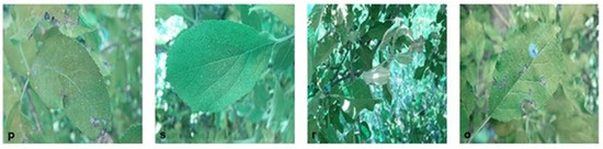
Figure 12.
Sample of Model_Lite’s optimal recognition accuracy.
The sample dataset shown in Figure 12 shows that the backgrounds of these four diseases were particularly complex, and the leaf diseases were almost integrated with the surrounding environment. Model_Lite could achieve a higher recognition accuracy in the four disease categories than the other network models. Combined with the heat map in Section 3.3, we found that this was mainly due to the model’s inclusion of the SE attention module between each lightweight residual module, which allowed for the extraction of features to strengthen the main disease features while ignoring the interference of irrelevant background factors.
4. Summary and Outlook
4.1. Summary
This study proposed a lightweight plant leaf disease recognition network model based on ResNet18, which addresses the issues of numerous parameters, extensive computation amounts, and complexity involved in recognition models. The proposed model improved the characteristics of the disease recognition process:
- First, a grouping convolution method was proposed, with the number of groups being equal to the number of channels in order to reduce the model size. The number of parameters in the improved model was approximately 1/46 of that in the original ResNet18 model, and the number of operations was approximately 1/11. Moreover, the average recognition accuracy was higher by 0.47%.
- We introduced the SE attention module to address the challenges in recognizing diseases with complex backgrounds. This module enhanced the interaction of information between grouped convolutional units and improved the model’s ability to extract the crucial features of the diseases. By incorporating the SE maximal grouping, the average recognition accuracy of the model was improved by 0.48%.
- To tackle the issue of losing disease features due to the low resolution of the feature map, the downsampling operation of the original network was removed in layer 3 and layer 4 of the model. This led to an increased resolution of the feature map of 28 × 28. Furthermore, a cavity volume was incorporated to maintain the exact size of the network’s receptive field. These modifications significantly enhanced the model’s performance. The average recognition accuracy of the maximum grouping model witnessed a 0.53% improvement, with only a slight increase in the computational effort required.
- Boosting the residual connection to make the feature extraction more comprehensive and intricate led to further enhancements in the model’s performance. The average recognition accuracy of the maximum grouping model was enhanced by 0.19%, while the same number of parameters and computational resources was maintained.
- Rational streamlining of the network models was achieved by reducing the number of convolutional kernels.
Model_Lite, the final model with fewer convolutional kernels, had 1/344 of the parameters and 1/35 of the computational effort of the original ResNet18 model. Despite a 0.34% decrease in the average accuracy on the experimental dataset, Model_Lite achieved the highest recognition accuracy of 91.21% compared to lightweight networks such as MobileNet, ShuffleNet, SqueezeNet, and GhostNet. Moreover, the number of parameters in the model and the computation amount were significantly less than those of the mainstream lightweight network models. Deploying the model to a mobile terminal could enable plant growers to conveniently identify diseases and minimize the economic losses resulting from untimely disease diagnosis. Additionally, this study’s improved methodology provides a reference for future research on lightweight network models.
4.2. Outlook
Although this study made some breakthroughs, challenges and limitations remain. The following are a few core issues we identified and some future research directions:
- Considering the relatively small number of complex background apple disease samples we constructed on our own, the learning potential of the model is still not fully unleashed. We plan to expand the dataset further to improve the model’s performance more comprehensively.
- As the resolution of the feature map increased, the recognition accuracy of the model was optimized, but the computational effort of the model also increased. For this reason, subsequent research will focus on this area, seeking strategies to reduce the computational cost while maintaining accuracy.
- Currently, our model has yet to be deployed on mobile platforms. This is an area to be developed, and in the future, we will focus on how to make it lightweight and optimize its performance for the mobile environment.
Author Contributions
Conceptualization, L.M.; data curation, Y.H.; formal analysis, Y.M.; funding acquisition, L.M.; project administration, G.C.; supervision, L.M.; validation, Y.H.; visualization, Z.L.; writing review and editing, L.M. and Y.H. All authors have read and agreed to the published version of the manuscript.
Funding
This work was supported by the National Natural Science Foundation of China Joint Fund (u19a2061), the Jilin Provincial Science and Technology Department Key Consultation Project (20210204050YY), the China Academy of Engineering Consultation Key Project (JL2023-03), the Jilin Provincial Natural Science Foundation (no. 20200201288JC), and the Jilin Provincial Development and Reform Commission Project (2021C044-4).
Data Availability Statement
Data supporting the findings of this study are available from the corresponding author.
Conflicts of Interest
The authors declare no conflict of interest.
References
- Wei, L.; Yue, J.; Li, Z.; Kou, G.; Qu, H. Multi-Classification Detection Method of Plant Leaf Disease Based on Dernel Function SVM. Trans. CSAM 2017, 48, 166–171. [Google Scholar]
- Bao, W.; Zhao, J.; Hu, G.; Zhang, D.; Huang, L.; Liang, D. Identification of Wheat Leaf Diseases and Their Severity Based on Elliptical-Maximum Margin Criterion Metric Learning. Sustain. Comput. Inform. Syst. 2021, 30, 100526. [Google Scholar] [CrossRef]
- Thanammal Indu, V.; Suja Priyadharsini, S. Crossover-Based Wind-Driven Optimized Convolutional Neural Network Model for Tomato Leaf Disease Classification. J. Plant Dis. Prot. 2022, 129, 559–578. [Google Scholar] [CrossRef]
- Keerthi, J.; Maloji, S.; Krishna, P.G. An Approach of Tomato Leaf Disease Detection Based on SVM Classifier. Int. J. Recent Technol. Eng. IJRTE 2019, 7. [Google Scholar]
- Yan, Z.; Qingxue, L.; Huarui, W. Rapid Recognition Model of Tomato Leaf Diseases Based on Kernel Mutual Subspace Method. Smart Agric. 2020, 2, 86. [Google Scholar]
- Yongquan, X.; Bing, W.; Jun, Z.; Haipeng, H.; Jingru, S. Identification of Wheat Leaf Disease Based on Random Forest Method. J. Graph. 2018, 39, 57. [Google Scholar]
- Wu, Y.; Wu, J.; Hu, G. MMFS: A Grape Disease Recognition Method Based on Multi-Feature Fusion and SVM. In Proceedings of the 2020 4th International Conference on Cloud and Big Data Computing, Virtual, 26–28 August 2020; pp. 27–31. [Google Scholar]
- Mokhtar, U.; Ali, M.A.S.; Hassanien, A.E.; Hefny, H. Identifying Two of Tomatoes Leaf Viruses Using Support Vector Machine. In Information Systems Design and Intelligent Applications; Mandal, J.K., Satapathy, S.C., Kumar Sanyal, M., Sarkar, P.P., Mukhopadhyay, A., Eds.; Advances in Intelligent Systems and Computing; Springer: New Delhi, India, 2015; Volume 339, pp. 771–782. ISBN 978-81-322-2249-1. [Google Scholar]
- Ma, L.; Zhao, L.; Wang, Z.; Zhang, J.; Chen, G. Detection and Counting of Small Target Apples under Complicated Environments by Using Improved YOLOv7-Tiny. Agronomy 2023, 13, 1419. [Google Scholar] [CrossRef]
- Sujatha, R.; Chatterjee, J.M.; Jhanjhi, N.Z.; Brohi, S.N. Performance of Deep Learning vs. Machine Learning in Plant Leaf Disease Detection. Microprocess. Microsyst. 2021, 80, 103615. [Google Scholar] [CrossRef]
- Zhang, J.; Huang, Y.; Pu, R.; Gonzalez-Moreno, P.; Yuan, L.; Wu, K.; Huang, W. Monitoring Plant Diseases and Pests through Remote Sensing Technology: A Review. Comput. Electron. Agric. 2019, 165, 104943. [Google Scholar] [CrossRef]
- Yang, G.; Chen, G.; He, Y.; Yan, Z.; Guo, Y.; Ding, J. Self-Supervised Collaborative Multi-Network for Fine-Grained Visual Categorization of Tomato Diseases. IEEE Access 2020, 8, 211912–211923. [Google Scholar] [CrossRef]
- Sun, X.; Wei, J. Identification of Maize Disease Based on Transfer Learning. In Proceedings of the Journal of Physics: Conference Series; IOP Publishing: Bristol, UK, 2020; Volume 1437, p. 012080. [Google Scholar]
- Yan, Q.; Yang, B.; Wang, W.; Wang, B.; Chen, P.; Zhang, J. Apple Leaf Diseases Recognition Based on an Improved Convolutional Neural Network. Sensors 2020, 20, 3535. [Google Scholar] [CrossRef] [PubMed]
- Wang, G.; Wang, J.; Yu, H.; Sui, Y. Research on Identification of Corn Disease Occurrence Degree Based on Improved ResNeXt Network. Int. J. Pattern Recognit. Artif. Intell. 2022, 36, 2250005. [Google Scholar] [CrossRef]
- Li, Y.; Han, Z.; Xu, H.; Liu, L.; Li, X.; Zhang, K. YOLOv3-Lite: A Lightweight Crack Detection Network for Aircraft Structure Based on Depthwise Separable Convolutions. Appl. Sci. 2019, 9, 3781. [Google Scholar] [CrossRef]
- Kc, K.; Yin, Z.; Wu, M.; Wu, Z. Depthwise Separable Convolution Architectures for Plant Disease Classification. Comput. Electron. Agric. 2019, 165, 104948. [Google Scholar] [CrossRef]
- Li, D.; Yang, C.; Yao, R.; Ma, L. Origin Identification of Saposhnikovia Divaricata by CNN Embedded with the Hierarchical Residual Connection Block. Agronomy 2023, 13, 1199. [Google Scholar] [CrossRef]
- Li, T.; Liu, L.; Li, M. Multi-Scale Residual Depthwise Separable Convolution for Metro Passenger Flow Prediction. Appl. Sci. 2023, 13, 11272. [Google Scholar] [CrossRef]
- He, K.; Zhang, X.; Ren, S.; Sun, J. Deep Residual Learning for Image Recognition. In Proceedings of the IEEE Conference on Computer Vision and Pattern Recognition, Las Vegas, NV, USA, 27–30 June 2016; pp. 770–778. [Google Scholar]
- Hu, J.; Shen, L.; Sun, G. Squeeze-and-Excitation Networks. In Proceedings of the IEEE Conference on Computer Vision and Pattern Recognition, Salt Lake City, UT, USA, 18–23 June 2018; pp. 7132–7141. [Google Scholar]
- Yu, F.; Koltun, V.; Funkhouser, T. Dilated Residual Networks. In Proceedings of the IEEE Conference on Computer Vision and Pattern Recognition, Honolulu, HI, USA, 21–26 July 2017; pp. 472–480. [Google Scholar]
- Hughes, D.; Salathé, M. An Open Access Repository of Images on Plant Health to Enable the Development of Mobile Disease Diagnostics. arXiv 2015, arXiv:151108060. [Google Scholar]
- Krizhevsky, A.; Sutskever, I.; Hinton, G.E. Imagenet Classification with Deep Convolutional Neural Networks. Adv. Neural Inf. Process. Syst. 2012, 25, 1097–1105. [Google Scholar] [CrossRef]
- Xie, S.; Girshick, R.; Dollár, P.; Tu, Z.; He, K. Aggregated Residual Transformations for Deep Neural Networks. In Proceedings of the IEEE Conference on Computer Vision and Pattern Recognition, Honolulu, HI, USA, 21–26 July 2017; pp. 1492–1500. [Google Scholar]
- Yang, L.; Yu, X.; Zhang, S.; Long, H.; Zhang, H.; Xu, S.; Liao, Y. GoogLeNet Based on Residual Network and Attention Mechanism Identification of Rice Leaf Diseases. Comput. Electron. Agric. 2023, 204, 107543. [Google Scholar] [CrossRef]
- Liao, T.; Yang, R.; Zhao, P.; Zhou, W.; He, M.; Li, L. MDAM-DRNet: Dual Channel Residual Network with Multi-Directional Attention Mechanism in Strawberry Leaf Diseases Detection. Front. Plant Sci. 2022, 13, 869524. [Google Scholar] [CrossRef]
- Xu, Y.; Gao, Z.; Zhai, Y.; Wang, Q.; Gao, Z.; Xu, Z.; Zhou, Y. A CNNA-Based Lightweight Multi-Scale Tomato Pest and Disease Classification Method. Sustainability 2023, 15, 8813. [Google Scholar] [CrossRef]
- Vaswani, A.; Shazeer, N.; Parmar, N.; Uszkoreit, J.; Jones, L.; Gomez, A.N.; Kaiser, L.; Polosukhin, I. Attention Is All You Need. Adv. Neural Inf. Process. Syst. 2017, 30. [Google Scholar] [CrossRef]
- Wang, Q.; Wu, B.; Zhu, P.; Li, P.; Zuo, W.; Hu, Q. ECA-Net: Efficient Channel Attention for Deep Convolutional Neural Networks. In Proceedings of the IEEE/CVF Conference on Computer Vision and Pattern Recognition, Seattle, WA, USA, 13–19 June 2020; pp. 11534–11542. [Google Scholar]
- Woo, S.; Park, J.; Lee, J.-Y.; Kweon, I.S. Cbam: Convolutional Block Attention Module. In Proceedings of the European Conference on Computer Vision (ECCV), Munich, Germany, 8–14 September 2018; pp. 3–19. [Google Scholar]
- Selvaraju, R.R.; Cogswell, M.; Das, A.; Vedantam, R.; Parikh, D.; Batra, D. Grad-Cam: Visual Explanations from Deep Networks via Gradient-Based Localization. In Proceedings of the IEEE International Conference on Computer Vision, Venice, Italy, 22–29 October 2017; pp. 618–626. [Google Scholar]
- Howard, A.G.; Zhu, M.; Chen, B.; Kalenichenko, D.; Wang, W.; Weyand, T.; Andreetto, M.; Adam, H. Mobilenets: Efficient Convolutional Neural Networks for Mobile Vision Applications. arXiv 2017, arXiv:170404861. [Google Scholar]
- Zhang, X.; Zhou, X.; Lin, M.; Sun, J. Shufflenet: An Extremely Efficient Convolutional Neural Network for Mobile Devices. In Proceedings of the IEEE Conference on Computer Vision and Pattern Recognition, Salt Lake City, UT, USA, 18–23 June 2018; pp. 6848–6856. [Google Scholar]
- Iandola, F.N.; Han, S.; Moskewicz, M.W.; Ashraf, K.; Dally, W.J.; Keutzer, K. SqueezeNet: AlexNet-Level Accuracy with 50× Fewer Parameters and <0.5 MB Model Size. arXiv 2016, arXiv:160207360. [Google Scholar]
- Han, K.; Wang, Y.; Tian, Q.; Guo, J.; Xu, C.; Xu, C. Ghostnet: More Features from Cheap Operations. In Proceedings of the IEEE/CVF Conference on Computer Vision and Pattern Recognition, Seattle, WA, USA, 13–19 June 2020; pp. 1580–1589. [Google Scholar]
- Ma, N.; Zhang, X.; Zheng, H.-T.; Sun, J. Shufflenet v2: Practical Guidelines for Efficient Cnn Architecture Design. In Proceedings of the European Conference on Computer Vision (ECCV), Munich, Germany, 8–14 September 2018; pp. 116–131. [Google Scholar]
Disclaimer/Publisher’s Note: The statements, opinions and data contained in all publications are solely those of the individual author(s) and contributor(s) and not of MDPI and/or the editor(s). MDPI and/or the editor(s) disclaim responsibility for any injury to people or property resulting from any ideas, methods, instructions or products referred to in the content. |
© 2023 by the authors. Licensee MDPI, Basel, Switzerland. This article is an open access article distributed under the terms and conditions of the Creative Commons Attribution (CC BY) license (https://creativecommons.org/licenses/by/4.0/).