Abstract
Computer vision provides a real-time, non-destructive, and indirect way of horticultural crop yield estimation. Deep learning helps improve horticultural crop yield estimation accuracy. However, the accuracy of current estimation models based on RGB (red, green, blue) images does not meet the standard of a soft sensor. Through enriching more data and improving the RGB estimation model structure of convolutional neural networks (CNNs), this paper increased the coefficient of determination (R2) by 0.0284 and decreased the normalized root mean squared error (NRMSE) by 0.0575. After introducing a novel loss function mean squared percentage error (MSPE) that emphasizes the mean absolute percentage error (MAPE), the MAPE decreased by 7.58%. This paper develops a lettuce fresh weight estimation method through the multi-modal fusion of RGB and depth (RGB-D) images. With the multimodal fusion based on calibrated RGB and depth images, R2 increased by 0.0221, NRMSE decreased by 0.0427, and MAPE decreased by 3.99%. With the novel loss function, MAPE further decreased by 1.27%. A MAPE of 8.47% helps to develop a soft sensor for lettuce fresh weight estimation.
1. Introduction
Precise climate control is vital for greenhouse crop growth. The greenhouse crop mechanistic model [1] is the basis for model predictive control [2] or optimal control [3]. One key factor hindering the application of the optimal control algorithm is the lack of reliable crop models and suitable on-line plant measurements [4]. Two direct measurement methods are destructive measurements and load cells. Destructive plant measurements [5] are time-consuming, influence the greenhouse climate, and harm the crop value. The high-cost load cells [6] are influenced by the water household of plants. An indirect measurement method is through a soft sensor based on a crop model. Xu et al. [7] developed a soft sensor for greenhouse lettuce dry mass based on a lettuce growth model. However, the soft sensor is only reliable when the lettuce growth model is perfect.
With the development of computer vision and artificial intelligence, a data-driven soft sensor based on crop images provides a new way of plant measurement. Van Henten and Bontsema [8] introduced image processing to detect lettuce growth in a full-scale experiment in a greenhouse. Three models that describe the relationship between the relative soil coverage by the crop canopy and dry weight were discussed. The predicted dry weights all fell into the 95% confidence interval. Machine learning methods through empirical feature extraction of RGB images [9,10,11,12,13,14] or 3D cloud images [15,16] showed promising estimation results of lettuce fresh weight. Zhang et al. [17] compared a convolutional neural network (CNN) with other machine learning methods in estimating lettuce fresh weight, dry weight, and leaf area for three cultivars. Results showed that the deep-learning-based CNN outperformed machine learning methods through RGB or depth images in estimating three lettuce growth traits for three cultivars. Machine learning methods usually require segmentation of the lettuce from its background and manually extracting features, while deep learning methods can automatically extract features from the whole image. However, Zhang et al. [17] did not explore the potential of RGB-D fusion in deep learning methods.
With the development of deep multimodal learning technology [18], some researchers explored its use in estimating lettuce fresh weight through an open dataset from the third Autonomous Greenhouse Challenge: Online Challenge (https://data.4tu.nl/articles/_/15023088/1, accessed on 1 January 2020). Buxbaum et al. [19] converted depth images into pseudo-color images and used a two-branch CNN composed of two ResNet-50 structures to estimate lettuce dry mass. Results found that depth images help in increasing the estimation accuracy, especially for small lettuces. Lin et al. [20] used U-Net to segment the lettuce and extract 10 geometric traits. A multi-branch regression network trained with RGB-D-G (Red, Green, Blue—Depth—Geometric) data outperformed networks with other combinations of data types. A root mean squared error (RMSE) of 25.3 g, a coefficient of determination (R2) of 0.938, and a mean absolute percentage error (MAPE) of 17.7% were found in their research. Zhang et al. [21] proposed a three-stage, multi-branch, self-correcting trait estimation network (TMSCNet) for RGB and depth images of lettuce. An R2 of 0.9514, which outperformed Lin et al. [20], was found in their research. The results of Lin et al. [20] and Zhang et al. [21] showed that the multimodal fusion of RGB-D images outperformed RGB images in deep learning methods.
In this paper, a new RDB-D fusion method that calibrates the RGD and depth images and then estimates the lettuce with a single CNN is raised. The proposed system can be run within 1 s. Considering the dynamics of lettuce growth and greenhouse climate, the latencies are negligible. The contributions are as follows: (1) The CNN structure is improved to estimate the lettuce fresh weight more accurately with an enriched RGB dataset. (2) A novel loss function that emphasizes MAPE is developed and verified. (3) Calibrations of RGB and depth images are performed to facilitate multimodal data fusion. (4) An RGB-D estimation model is developed to decrease the MAPE to 8.47%, which helps to develop the soft sensor that can estimate the lettuce fresh weight with a relatively high accuracy of over 90%.
2. Materials and Methods
2.1. RGB and RGB-D Data Acquisition
To improve the estimation accuracy of lettuce fresh weight based on the original RGB dataset, the 286 RGB and depth images of lettuces in three cultivars (Flandria, Tiberius, and Locarno) with three growth traits (fresh weight, dry weight, and leaf area) used by Zhang et al. [17] are downloaded from the open dataset (https://figshare.com/authors/Juncheng_Ma/8733486, accessed on 1 January 2020).
To improve the estimation accuracy of lettuce fresh weight with an enriched RGB dataset, field measurements were performed in a similar experimental setup. Because the estimation accuracy of lettuce fresh weight is the highest with the cultivar “Tiberius” [17], only “Tiberius” lettuces were planted in the same greenhouse as Zhang’s [17], as shown in Figure 1. The RGB and depth images were collected with the same Kinect 2.0, and lettuce fresh weights were sampled during 9:00–12:00 every Friday from 6 December 2019 to 10 January 2020. After this round of field measurements, 200 more lettuce fresh weights with RGB and depth images were collected and uploaded to the same open dataset; so, there are 486 RGB images in the enriched RGB dataset. The ground truth of lettuce fresh weight is measured by an electronic balance with the precision of 0.01 g after root removal.
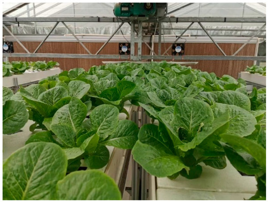
Figure 1.
Picture of the experimental greenhouse.
The depth data of Kinect 2.0 are only valid at heights between 0.5 and 4.5 m. A schematic diagram and a field picture of the sampling device are shown in Figure 2. We can see from the schematic diagram that the depth data are only valid when the lettuce is lower than 17.5 cm. So, some depth data from the open dataset are not valid, especially for those tall lettuces.
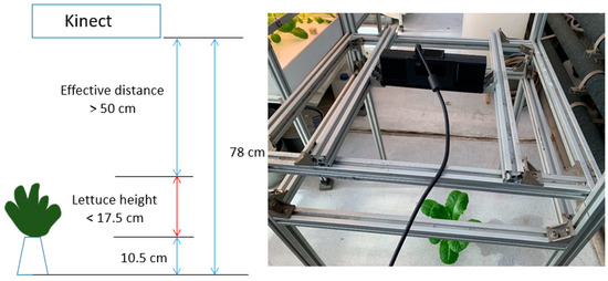
Figure 2.
A schematic diagram and a field picture of the sampling device.
An example of the invalid depth data is shown in Figure 3. The pixels that have no value are shown in black. We can see from Figure 3 that a lot of pixels in the leaves are not valid; these data should be removed from the RGB-D dataset. In this paper, the RGB-D data with amounts of pixels that have no depth value within the lettuce canopy area are regarded as invalid.
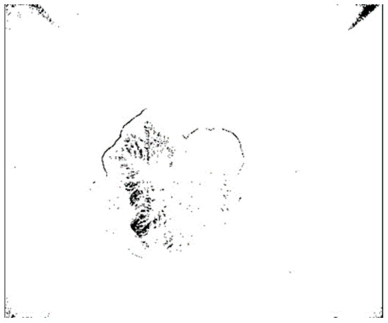
Figure 3.
An example of invalid depth data.
After removal, only RGB-D data of 366 lettuces are left. The distributions of lettuce fresh weights for 486 RGB images and 366 RGB-D images are shown in Figure 4. We can see that those lettuces heavier than 120 g are all removed in the RGB-D dataset.
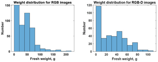
Figure 4.
Distributions of lettuce fresh weights for 486 RGB images and 366 RGB-D images.
From Table 1, we can have a clear view of the number of images with different cultivars in the original RGB dataset, the enriched RGB dataset, and the RGB-D dataset. One should note that fewer “Locarno” lettuces are removed in the RGB-D dataset because they are smaller than lettuces in the other two cultivars [17].

Table 1.
Numbers of images in different datasets.
2.2. RGB-D Calibration
Kinect 2.0 is composed of an RGB camera, an infrared camera, and an infrared projector. Depth data are obtained through the infrared camera with Time of Flight (TOF) technology. Calibration is needed in image registration for RGB-D fusion. The calibration of the Kinect 2.0 for the measurement experiment is performed with the method of Zhang [22]. The calibration plate is printed with the 16:9 checkerboard composed of 30 mm × 30 mm checks. A total of 30 RGB images and 30 infrared images of the calibration plate with different poses are simultaneously collected with Kinect 2.0 at a fixed position, as shown in Figure 5.
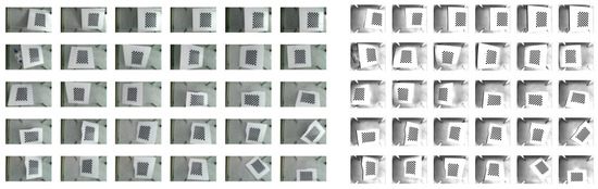
Figure 5.
RGB images and 30 infrared images of the calibration plate with different poses.
The calibration is performed with the Matlab toolbox “Camera Calibrator”. The mean reprojection errors of the RGB camera and infrared camera are 0.19 pixels and 0.07 pixels, respectively. A mean reprojection error of lower than 0.5 pixels is a guarantee of a good calibration.
The transformation from infrared coordinates to RGB coordinates is shown in Equation (1). , , and are horizontal coordinates, vertical coordinates, and depth values, respectively, of the camera coordinate system for RGB and infrared cameras. for RGB and infrared cameras is calculated in Equation (2) [22]. of the experimented Kinect 2.0 is shown in Equation (3).
The performance of RGB-D fusion is shown in Figure 6. The black points around the lettuce are invalid pixels from the depth images. Although this is an invalid sample, we can see that the outline of lettuce from the depth image has a relatively good fit with the outline from the RGB image. One should note that an invalid sample, not a valid sample, is shown in Figure 6 because the black points in the invalid sample can show the outline of the lettuce more clearly, while in a valid sample, few black points can be found in the fused RGB-D data.
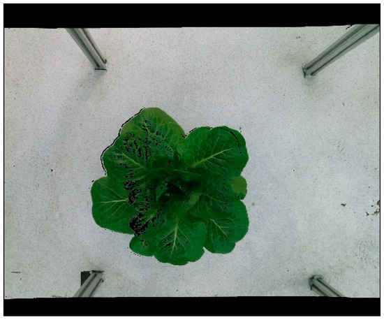
Figure 6.
The performance of RGB-D fusion.
2.3. Image Processing
After RGB-D fusions of 366 valid samples, the size of each sample becomes 512 × 424 × 4. After cropping each sample based on the center pixel, the size becomes 300 × 300 × 4. The 4 means red, green, blue, and depth values at each pixel. Parts of the fused data have no RGB values, as shown in Figure 6, because the length–width ratios in RGB and depth images are different. These parts are removed after the cropping. Then, the method of bilinear interpolation is used to adjust the RGB or RGB-D images to different sizes according to the input requirements of different CNN estimation models.
After cropping, the RGB-D samples are randomly divided into a training dataset, a validation dataset, and a test dataset with a ratio of 8:1:1, resulting 294 samples in the training dataset, 36 samples in the validation dataset, and 36 samples in the test dataset. One should note that the ratio of the original RGB datasets for training, validation, and testing remains the same as Zhang’s [17] at 6.4:1.6:2 for better comparisons. The ratio of RGB-D data for training is higher because there are fewer images compared with the enriched RGB dataset, as shown in Table 1. In the enriched RGB dataset, supplemented data are all used for training.
The training dataset and the validation dataset are augmented 26 times with the method shown in Zhang et al. [17]. A flow chart of augmentation is shown in Figure 7. The original image is rotated 90, 180, and 270 degrees, and flipped horizontally and vertically. Then, the brightness is adjusted to 80%, 90%, 110%, and 120%. This results in 7644 augmented samples in the training dataset and 936 augmented samples in the validation dataset for RGB-D data. The difference is that when RGB images change their brightness, depth data remain the same. However, depth images rotate and flip with RGB images.
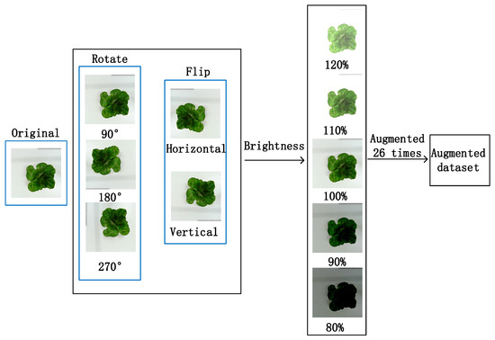
Figure 7.
Augmentation.
2.4. A Novel Loss Function That Emphasizes MAPE
The most used loss function in machine learning is the mean squared error (MSE) as shown in Equation (4), which is also used in training most of our CNNs. We should note that the loss function of MSE cannot guarantee the minimization of relative error. So, to develop a soft sensor, the MAPE—as shown in Equation (5)—should be the index that evaluates the performance of the estimation model. To this end, a novel loss function Mean Squared Percentage Error (MSPE) that emphasizes MAPE is developed in this paper, as shown in Equation (6). In Equations (4)–(6), m means the number of samples, Si means the true value per sample, and Ei means the estimation value per sample.
We should note that MAPE cannot be the loss function because the absolute-value sign shown in Equation (5) leads to difficulties in calculating the derivatives at those points where +/− signs change. So, the loss function of MSPE shown in Equation (6) that calculates the sum of squares per relative error is developed. Although MSPE is different from MAPE, it emphasizes MAPE better than MSE does, as we can see in Section 3.1.3.
2.5. Computing Environment
All CNN models are trained with the Pytorch deep learning framework. These computer experiments are performed on a Dell T5820 workstation (CPU: I9-10980XE @ 3.0 GHz, GPU: NVIDIA GeForce RTX A6000 with 48 GB memory).
3. Results and Discussion
3.1. Improve the Estimation Accuracy Based on RGB Data
The estimation accuracy based on RGB data is improved in three ways: (1) Explore the potential through enriching the dataset without changing the original model structure of Zhang et al. [17]. (2) Improve the model structure with the enriched dataset. (3) Improve the estimation accuracy through the novel loss function with the enriched dataset and the improved model structure.
3.1.1. Enrich the RGB Data
The original CNN model of Zhang et al. [17] was trained with lettuces in three cultivars to estimate three growth traits. To explore the potential of improving the estimation accuracy of lettuce fresh weight with the enriched dataset, the following experiments are performed, as shown in Table 2. One should note that all estimation results are based on the original “Tiberius” lettuces in the test dataset. IXOX means X cultivars and X growth traits. _Enrich means to train the CNN model with the enriched dataset. The number of epochs (300) and the mini-batch size (128) remain the same with Zhang et al. [17], while the optimizer Adam is used in this paper for better optimization. Except for R2 and NRMSE, which are used by Zhang et al. [17], the learning rate of each experimental setup is also shown in Table 2. NRMSE is calculated in Equation (7).
Table 2.
Estimation results of different experimental setups.
I3O3 shows the reproduction of the original experimental setup [17]. By comparing I3O3 and I3O1, we can see a clear increase in the estimation accuracy of lettuce fresh weight. By comparing with I3O1, one wants to expect an increase in the estimation accuracy in I1O1. However, the decrease in the estimation accuracy is a result of a smaller dataset (286 vs. 94). By comparing with I3O1, we can see a slight increase in the estimation accuracy in I1O1_enrich. The sizes of their datasets are comparable (286 vs. 294). The increase in the estimation accuracy in I1O1_enrich is a result of the supplemented “Tiberius” lettuces. So, when the sizes of the datasets are comparable, it is better to choose the dataset with the same cultivar if one wants to estimate the lettuce fresh weight of this cultivar more accurately.
From Table 3, we can see the estimation results for more cultivars. One should note that the results of I3O1 in Table 3, different from those in Table 2, are based on the original test dataset with three cultivars from Zhang et al. [17]. I3O1_enrich is performed by adding the supplemented “Tiberius” lettuce data into the training dataset while keeping the validation and the test dataset the same.
Table 3.
Estimation results with three cultivars.
We can see from Table 3 that if one wants to estimate lettuce fresh weight with three cultivars, it is better to have a larger dataset. The enriched dataset is used to improve the CNN model structure in Section 3.1.2.
3.1.2. Improve the Model Structure
The explored CNN structures are CNN_Zhang [17], VGG16 [23], ResNet18 [24], MobileNetV3_small [25], EfficientNetV2_small [26], and two improved CNNs based on CNN_Zhang. CNN_140 originates from removing the padding part of CNN_Zhang. CNN_284, as shown in Figure 8, originates from adding one more convolutional layer and one more padding layer to CNN_140. The estimation results of different CNNs are shown in Table 4. One should note that the mini-batch size of 96 for VGG16 is different from the mini-batch size of 128 for other CNN structures because of the heavy computation load.
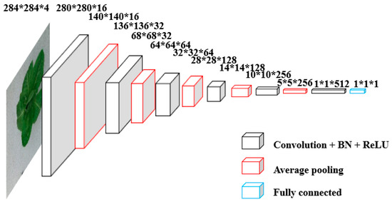
Figure 8.
The structure of CNN_284.
Table 4.
Estimation results of different CNNs with RGB images.
By comparing the results with Zhang et al. [17], we can see that R2 increases by 0.0212 and NRMSE decreases by 0.0315. This is because of the extra 200 samples and the estimation of only the lettuces’ fresh weight. We can also see that only CNN_284 outperforms CNN_Zhang, with R2 increasing by 0.0045 and NRMSE decreasing by 0.0061. The more sophisticated VGG16, ResNet18, MobileNet, and Efficient Net all face the problem of over-fitting. The improved performance of CNN_284 is a result of more samples and stronger feature extraction ability with one more convolutional layer. So, the model structure has to coordinate with the corresponding data size and task complexity.
3.1.3. Improve the Loss Function
With the novel loss function, as depicted in Section 2.4, the estimation results based on the best CNN structure are shown in Table 5. For comparison, the MAPE of CNN_284 with the loss function of MSE is also shown in Table 5.
Table 5.
Estimation results to compare MAPE.
We can see a clear decrease of 7.58% in MAPE caused by the loss function of MSPE. Although there is a slight decrease in R2 and a slight increase in NRMSE, the distinct decrease in MAPE is important if one wants to develop a soft sensor based on RGB data. However, the MAPE of higher than 10% is still far from the requirements of a soft sensor. In Section 3.2, we will try to further decrease MAPE based on RGB-D data.
3.2. Improve the Estimation Accuracy Based on RGB-D Data
With the RGB-D data, as depicted in Section 2.1, the estimation results of different CNNs with the loss function of MSE are shown in Table 6. For comparison of CNNs with RGB data and RGB-D data, CNN_Zhang results with the same 366 RGB images are also shown in Table 6. CNN_140, CNN_284, and CNN_572 are explored for estimating lettuce fresh weight with RGB-D data. CNN_572 originates from adding one more convolutional layer and one more padding layer to CNN_284. To see the influence of the novel loss function MSPE on RGB-D data, the results with the best CNN structure are also shown in Table 6.
Table 6.
Estimation results of different CNNs with RGB and RGB-D images.
By comparing CNN_Zhang in Table 6 with CNN_284_MSPE in Table 5, we can see a decrease of 0.62% in MAPE for estimating with RGB-D data, even without the novel loss function MSPE. This is because several RGB images are removed from the enriched dataset due to invalid corresponding depth data, as shown in Figure 4. The distribution of lettuce fresh weights from the remaining 366 images is more centralized.
CNN_284 shows the lowest MAPE of 9.74% based on RGB-D data with the loss function of MSE. Compared with CNN_Zhang based on RGB images, a decrease of 3.99% in MAPE can be found. This shows the strong power of RGB-D data fusion for lettuce fresh weight estimation. CNN_284 outperforms CNN_140 and CNN_572 for estimating lettuce fresh weights with RGB-D data. This proves that too deep or shallow structures of CNNs will not lead to a good estimation performance. Although a MAPE of lower than 10% is already friendly to a soft sensor, further decreases can be explored with the loss function MSPE.
By comparing CNN_284 and CNN_284_MSPE, we can see a decrease of 1.27% in MAPE with the novel loss function MSPE. This proves that the novel loss function MSPE is also powerful in decreasing MAPE for RGB-D data. The measured and estimated lettuce fresh weights of CNN_284_MSPE are shown in Figure 9. We can see that the relative errors for the whole lettuce growing period are low.
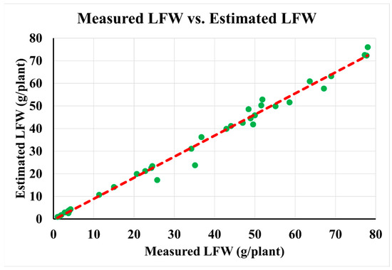
Figure 9.
Measured and estimated lettuce fresh weights of CNN_284_MSPE.
One should note that the MAPE of 8.47% should be tested for a larger dataset with more cultivars to develop a more comprehensive soft sensor in an optimally controlled greenhouse. The precision of within 10% is thought to meet the standard of a soft sensor for lettuce fresh weight. Although the RGB-D dataset is already enriched to be larger than the original RGB dataset, it is still advisable to further increase the number of images in the future. It is planned to be tested in a larger dataset in the future.
In optimal control of greenhouse climate, the sensitivity of profit is higher in lettuce growth model parameters than greenhouse climate model parameters [27]. Therefore, the feedback of lettuce yield is very important for the adaptive optimal control with varying lettuce model parameters [28]. Without this feedback, estimation error based on the lettuce growth model can be up to 34% [7]. With the perfect measurement of lettuce yield, profit can be increased by 24.5% [7]. Approximately, an improvement of 1% in the precision of lettuce yield estimation leads to an increase of 0.72% in profit of optimal control of greenhouse cultivation. As the non-contact indirect measurement of lettuce yield is still in its infancy, the soft sensor of lettuce yield with an MAPE of lower than 10% leads to an increase of approximately 7.2% in profit. For this reason, a MAPE of lower than 10% is a good standard for developing the soft sensor.
4. Conclusions
- 1.
- The estimation accuracy of lettuce fresh weight is improved based on RGB data in three ways: data enrichment, structure improvement, and loss function. Through data enrichment, R2 increases by 0.0284 and NRMSE decreases by 0.0575 if we only look at the cultivar “Tiberius”. If we look at three cultivars, the improvements are slight (R2 increases by 0.0058 and NRMSE decreases by 0.0082) because of data saturation. Through structure improvement, R2 increases by 0.0045 and NRMSE decreases by 0.0061. Through the novel loss function MSPE, MAPE decreases by 7.58%.
- 2.
- Different from the two-branch CNN, a new method that performs RGB-D fusion and estimates using a single-branch CNN is raised. The mean reprojection errors of 0.19 pixels and 0.07 pixels for the RGB camera and infrared camera, respectively, guarantee a relatively good calibration.
- 3.
- The improved CNN structure with RGB-D data outperforms CNNs with RGB images in estimating lettuce fresh weights. R2 increases by 0.0221, NRMSE decreases by 0.0427, and MAPE decreases by 3.99%. A MAPE of 8.47% is realized with the loss function MSPE. The MAPE of lower than 10% helps to develop a soft sensor for crop state feedback in optimal control of greenhouse climate.
Author Contributions
Conceptualization, D.X., J.C. and J.M.; methodology, D.X. and J.C.; experiments, J.C. and B.L.; resources, D.X. and J.M.; writing—original draft preparation, D.X. and J.C.; writing—review and editing, D.X., J.C. and J.M. All authors have read and agreed to the published version of the manuscript.
Funding
This work was financially supported by projects of the Key R&D Program of Shandong Province, China (2022CXGC020708); National Natural Science Foundation of China (32371998); National Modern Agricultural Technology System Construction Project (CARS-23-D02); and Beijing Innovation Consortium of Agriculture Research System (BAIC01-2023).
Informed Consent Statement
Not applicable.
Data Availability Statement
https://figshare.com/authors/Juncheng_Ma/8733486 (accessed on 8 October 2021).
Conflicts of Interest
The authors declare no conflict of interest.
References
- Righini, I.; Vanthoor, B.; Verheul, M.J.; Naseer, M.; Maessen, H.; Persson, T.; Stanghellini, C. A greenhouse climate-yield model focussing on additional light, heat harvesting and its validation. Biosyst. Eng. 2020, 194, 1–15. [Google Scholar] [CrossRef]
- Lin, D.; Zhang, L.; Xia, X. Model predictive control of a Venlo-type greenhouse system considering electrical energy, water and carbon dioxide consumption. Appl. Energy 2021, 298, 117163. [Google Scholar] [CrossRef]
- Xu, D.; Li, Y.; Dai, A.; Zhao, S.; Song, W. Closed-Loop Optimal Control of Greenhouse Cultivation Based on Two-Time-Scale Decomposition: A Simulation Study in Lhasa. Agronomy 2023, 13, 102. [Google Scholar] [CrossRef]
- Van Beveren, P.J.M.; Bontsema, J.; Van Straten, G.; Van Henten, E.J. Minimal heating and cooling in a modern rose greenhouse. Appl. Energy 2015, 137, 97–109. [Google Scholar] [CrossRef]
- Van Henten, E.J. Greenhouse Climate Management: An Optimal Control Approach; Wageningen University and Research: Wageningen, The Netherlands, 1994. [Google Scholar]
- Chen, W.T.; Yeh, Y.H.F.; Liu, T.Y.; Lin, T.T. An automated and continuous plant weight measurement system for plant factory. Front. Plant Sci. 2016, 7, 392. [Google Scholar] [CrossRef]
- Xu, D.; Du, S.; Van Willigenburg, G. Double closed-loop optimal control of greenhouse cultivation. Control. Eng. Pract. 2019, 85, 90–99. [Google Scholar] [CrossRef]
- Van Henten, E.J.; Bontsema, J. Non-destructive crop measurements by image processing for crop growth control. J. Agric. Eng. Res. 1995, 61, 97–105. [Google Scholar] [CrossRef]
- Lee, J.W. Machine vision monitoring system of lettuce growth in a state-of-the-art greenhouse. Mod. Phys. Lett. B 2008, 22, 953–958. [Google Scholar] [CrossRef]
- Yeh, Y.H.F.; Lai, T.C.; Liu, T.Y.; Liu, C.C.; Chung, W.C.; Lin, T.T. An automated growth measurement system for leafy vegetables. Biosyst. Eng. 2014, 117, 43–50. [Google Scholar] [CrossRef]
- Jung, D.H.; Park, S.H.; Han, X.Z.; Kim, H.J. Image processing methods for measurement of lettuce fresh weight. J. Biosyst. Eng. 2015, 40, 89–93. [Google Scholar] [CrossRef]
- Jiang, J.S.; Kim, H.J.; Cho, W.J. On-the-go image processing system for spatial mapping of lettuce fresh weight in plant factory. IFAC Pap. 2018, 51, 130–134. [Google Scholar] [CrossRef]
- Nagano, S.; Moriyuki, S.; Wakamori, K.; Mineno, H.; Fukuda, H. Leaf-movement-based growth prediction model using optical flow analysis and machine learning in plant factory. Front. Plant Sci. 2019, 10, 227. [Google Scholar] [CrossRef]
- Reyes-Yanes, A.; Martinez, P.; Ahmad, R. Real-time growth rate and fresh weight estimation for little gem romaine lettuce in aquaponic grow beds. Comput. Electron. Agric. 2020, 179, 105827. [Google Scholar] [CrossRef]
- Hu, Y.; Wang, L.; Xiang, L.; Wu, Q.; Jiang, H. Automatic non-destructive growth measurement of leafy vegetables based on kinect. Sensors 2018, 18, 806. [Google Scholar] [CrossRef]
- Mortensen, A.K.; Bender, A.; Whelan, B.; Barbour, M.M.; Sukkarieh, S.; Karstoft, H.; Gislum, R. Segmentation of lettuce in coloured 3D point clouds for fresh weight estimation. Comput. Electron. Agric. 2018, 154, 373–381. [Google Scholar] [CrossRef]
- Zhang, L.; Xu, Z.; Xu, D.; Ma, J.; Chen, Y.; Fu, Z. Growth monitoring of greenhouse lettuce based on a convolutional neural network. Hortic. Res. 2020, 7, 124. [Google Scholar] [CrossRef] [PubMed]
- Ramachandram, D.; Taylor, G.W. Deep multimodal learning: A survey on recent advances and trends. IEEE Signal Process. Mag. 2017, 34, 96–108. [Google Scholar] [CrossRef]
- Buxbaum, N.; Lieth, J.H.; Earles, M. Non-destructive plant biomass monitoring with high spatio-temporal resolution via proximal RGB-d imagery and end-to-End deep learning. Front. Plant Sci. 2022, 13, 758818. [Google Scholar] [CrossRef]
- Lin, Z.; Fu, R.; Ren, G.; Zhong, R.; Ying, Y.; Lin, T. Automatic monitoring of lettuce fresh weight by multi-modal fusion based deep learning. Front. Plant Sci. 2022, 13, 980581. [Google Scholar] [CrossRef]
- Zhang, Q.; Zhang, X.; Wu, Y.; Li, X. TMSCNet: A three-stage multi-branch self-correcting trait estimation network for RGB and depth images of lettuce. Front. Plant Sci. 2022, 13, 982562. [Google Scholar] [CrossRef]
- Zhang, Z. A flexible new technique for camera calibration. IEEE Trans. Pattern Anal. Mach. Intell. 2000, 22, 1330–1334. [Google Scholar] [CrossRef]
- Simonyan, K.; Zisserman, A. Very deep convolutional networks for large-scale image recognition. arXiv 2014, arXiv:1409.1556. [Google Scholar]
- He, K.; Zhang, X.; Ren, S.; Sun, J. Deep residual learning for image recognition. Proc. IEEE Conf. Comput. Vis. Pattern Recognit. 2016, 97, 770–778. [Google Scholar]
- Howard, A.G.; Zhu, M.; Chen, B.; Kalenichenko, D.; Wang, W.; Weyand, T.; Adam, H. Mobilenets: Efficient convolutional neural networks for mobile vision applications. arXiv 2017, arXiv:1704.04861. [Google Scholar]
- Tan, M.; Le, Q. Efficientnet: Rethinking model scaling for convolutional neural networks. Int. Conf. Mach. Learn. 2019, 6105–6114. [Google Scholar]
- Van Henten, E.J. Sensitivity Analysis of an Optimal Control Problem in Greenhouse Climate Management. Biosyst. Eng. 2003, 85, 355–364. [Google Scholar] [CrossRef]
- Xu, D.; Du, S.; Van Willigenburg, L.G. Adaptive two time-scale receding horizon optimal control for greenhouse lettuce cultivation. Comput. Electron. Agric. 2018, 146, 93–103. [Google Scholar] [CrossRef]
Disclaimer/Publisher’s Note: The statements, opinions and data contained in all publications are solely those of the individual author(s) and contributor(s) and not of MDPI and/or the editor(s). MDPI and/or the editor(s) disclaim responsibility for any injury to people or property resulting from any ideas, methods, instructions or products referred to in the content. |
© 2023 by the authors. Licensee MDPI, Basel, Switzerland. This article is an open access article distributed under the terms and conditions of the Creative Commons Attribution (CC BY) license (https://creativecommons.org/licenses/by/4.0/).