Web Mapping for Farm Management Information Systems: A Review and Australian Orchard Case Study

Abstract

A web mapping XYZ Tile Layer Service, such as Google Earth (GE), provides an amazing resource for the visualization of spatial data against aerial and satellite imagery with global coverage, typically at a resolution finer than 5 m. However, the increasing requirement on spatial accuracy in farm information requires a greater appreciation of the issues involved in the use of such services. Position errors can be created in the georeferencing and orthorectification of images, transformation between reference frames (datums) in map projection, e.g., using a spheroid as compared to an ellipsoid earth model, and tectonic shifts. A review is provided of these issues, and a case study is provided of the horizontal positional accuracy of web map imagery for Australian mango orchards. Positional accuracies varied from 1.804 to 6.131 m across four farms using GE 2021 imagery, between 1.556 and 3.365 m in one farm for the most recent imagery available from each of four web map providers, and from 0.806 m (in 2016) to 10.634 m (in 2003) in one farm for the period of 2003 and 2021 using the historical GE imagery resource. A procedure involving the estimation of four transformation parameters was demonstrated for the alignment of GNSS data with GE imagery. However, as the scale factor was unity and the rotational value was near zero, the use of a simple horizontal mean shift vector was recommended. Further recommendations are provided on (i) the use of web mapping services, with a comparison of the use of UAV survey imagery, and (ii) the need for metadata, particularly the date of collection, on collected position data, in the context of use in farm management information systems.

1. Introduction

Context

Current Global Navigation Satellite System (GNSS)-based geodetic techniques allow up to millimeter accuracy in positioning to be achieved globally, and high-precision mass-market positioning is becoming available to an accuracy of 5–10 cm [1]. In the case of ‘build it and they will come’, many applications have been built on this GNSS capacity, with applications increasingly requiring higher positioning accuracy [2,3]. For example, auto-steer guidance of tractors has enabled controlled traffic in broadacre cropping, with vehicles following the same wheel tracks within a few centimeters to limit soil compaction [4], and UAV imagery can be used to map the position of small weeds for ground platform-based precision spraying [5]. GNSS-enabled applications are also developing in row and tree crop horticulture, e.g., linking chemical spray intensity for flowering thinning to machine vision and learning measurements of flower density [6] and the detection of weeds in real time [7].

With an increase in spatially tagged data comes a need to visualize such data, as seen in commercial farm management information systems (FMIS). Web mapping resources, such as Google Maps, provide an interactive display of geographic data and information in the form of a web page, enabling access from any internet-connected device [8]. Given their ubiquitous availability, web mapping resources are commonly used in FMIS, e.g., for denoting plot boundaries (e.g., for apple orchards [9]), displaying data (e.g., location of sensors for pest detection [10]), management functions (e.g., irrigation, [11]), and interpretation of data (e.g., geochemical data [12]). Most commercially available FMIS use web map resources, e.g., onside.com.nz (accessed on 3 July 2023); https://www.datafarming.com.au/ (accessed on 3 July 2023).

However, while position data can be very accurately assessed using GNSS services and tagged to field collected data, their accuracy can also be degraded in storage, processing, and delivery [13]. Indeed, the geodetic field is in a state of flux as the availability and use of high spatial resolution data increases.

Given the expanding uses for sub-meter spatial resolution in agricultural applications, it is timely to summarize the technologies behind spatial data collection (‘geodesy’) and web mapping and consider limitations in the use of these resources in the context of use in FMIS. A history and description of GNSS technology and datums, web mapping, and the source of positional error is presented in Section 2, serving as a tutorial for researchers seeking to visualize geolocated data. The impact of approximations that are routinely made is also described, including those incurred in moving between reference frames and in the use of web mapping, including ellipsoid to spheroid conversion, georeferencing, and orthorectification errors. A case study involving Australian mango orchards is presented in Section 3 and Section 4, documenting positional errors associated with web maps. This case study arises from our need to process and display machine vision-derived flower and fruit counts collected at multiple time points for entire orchards [3]. In this application, positional accuracy to around 1 m is required to maintain data at the ‘tree level’. Section 4.5 provides recommendations on the procedures required to maintain positional accuracy for records collected across time within FMIS. Definition of terminologies used are listed in Appendix A. The manuscript structure is not that of a classic ‘review’; however, we believe this resource will be very useful to others working in this field.

2. Background

2.1. A Primer on the GNSS

The Global Positioning System (GPS) was first operationalized by the U.S. Department of Defense in 1978, although its satellite constellation was not fully complete until 1995. The Russian GLONASS, European Galileo, and Chinese BeiDou systems achieved full operational capability in 1995, 2021, and 2020, respectively, albeit functioning at a range of position accuracies and levels of global coverage. The four systems are collectively referred to as Global Navigation Satellite Systems (GNSS). The GPS system was originally restricted to military use until the Reagan administration allowed degraded civilian use following the destruction of a Korean Airlines passenger plane that strayed into Russian airspace in 1983. The Clinton administration allowed civilian access to un-degraded GPS signals in 2000, and this commitment was made permanent in 2007 [14]. Civilian access to data from GLONASS and BeiDou geo-positioning systems has followed. Galileo access was always open, as it was the only non-military system.

The data sampling rate (also known as the update rate) of a GNSS module is the rate at which the position is calculated and reported. This is determined by both the satellite constellation accessed and the receiver chipset quality, with the primary limitation being the computing power of the receiver [15]. The GPS constellation outputs data at 1000 Hz. However, many receivers support only a 1 Hz rate, although receivers with update rates of 5, 10, and 20 Hz are available. A 1 Hz rate is adequate for non-moving applications. This specification is important to agricultural applications involving moving vehicles. For example, the orchard imaging system described by Anderson et al. [6] captures geolocated images at 10 fps from a ground vehicle moving at 7 km/h, i.e., 1.9 m/s. The matching of frame capture time to location data collected at this rate or higher will require interpolation of GNSS data.

A single point receiver (also referred to as a standalone receiver) of GNSS data has a positioning error of 5–10 m because of fluctuations in the GNSS signal due to variations in the layers of the atmosphere, multipath signals, and receiver electrical noise, in addition to errors in satellite clocks and imperfect satellite orbits. In differential GNSS (DGNSS), data are collected from a reference (base) station(s) at a known location, with the estimated position error on the reference station used to adjust the estimated rover position. Real-time kinematics (RTKs) also use base station data but employ more sophisticated algorithms, correcting ionospheric changes and satellite clock errors. Position accuracies of DGNSS and RTK are approx. 0.5 m and 0.02 m, respectively. In Australian surveying practice, the use of DGPS supported by local base stations has been largely replaced by the use of RTK based on a public/private network of Continuously Operating Reference Stations (CORS). However, a data link is required to access the CORS-RTK service in real time, and internet or 4G cellular service has been limited in agricultural areas.

The satellite-based augmentation system (SBAS, also known as wide-area differential GNSS) is an alternative that is widely adopted in Australian broadacre agriculture. In SBAS, a satellite signal is used to provide correction for satellite orbits and clocks, and information on the signal delay incurred in passes through the ionosphere that is calculated from multiple base stations. Such systems achieve a horizontal position 1 sigma accuracy below 1 m. Major agricultural technology providers such as John Deere (Moline, Illinois, United States), Case (Turin, Italy), Ag Leader (Ames, Iowa, United States), and Trimble (Westminister, Colorado, United States) have relied on the Inmarsat-4 constellation of three high-orbit satellites to deliver the correction data. However, the F-1 satellite that services Australasia has had several outages since its launch in 2005, including in March 2023 when two-thirds of the Australian winter wheat seeding program was reported to be impacted [16].

Precise point positioning (PPP) uses the ‘direct observables’ of dual frequencies broadcast by satellites (L1 and L2 in the case of GPS) to estimate ionospheric change and ‘ephemerides’ data, which are precise estimates of satellite orbits estimated using data from a global network of ground stations. Post-processing solutions have been available to implement corrections based on such estimates, but recently improved ephemerides data have become available with low latency over the internet. For example, an open-source toolkit (‘Ginan’) has recently been released for the creation of precise point positioning (PPP) positions and analysis products in Australia [17]. This free resource can be used in local applications with 4 or 5G service or an internet connection to deliver position correction data, providing positioning accuracy to 3 to 5 cm across Australia [17]. It is anticipated that in the future, consumer-level devices will access this service to deliver a highly accurate positioning capability. However, PPP requires more processing power than conventional methods and connectivity for access to an ephemeris correction stream, and it can take longer (minutes to hour) to converge to full accuracy.

The recent development of the Starlink communication satellite constellation (Starlink, Redmond, Washington, USA) is dramatically changing connectivity, offering (Australian) continent-wide coverage in a reliable, low-cost solution. This resource currently consists of 3580, of a planned 12,000, low-orbit satellites. This capacity can underpin the delivery of SBAS, RTK, or PPP services.

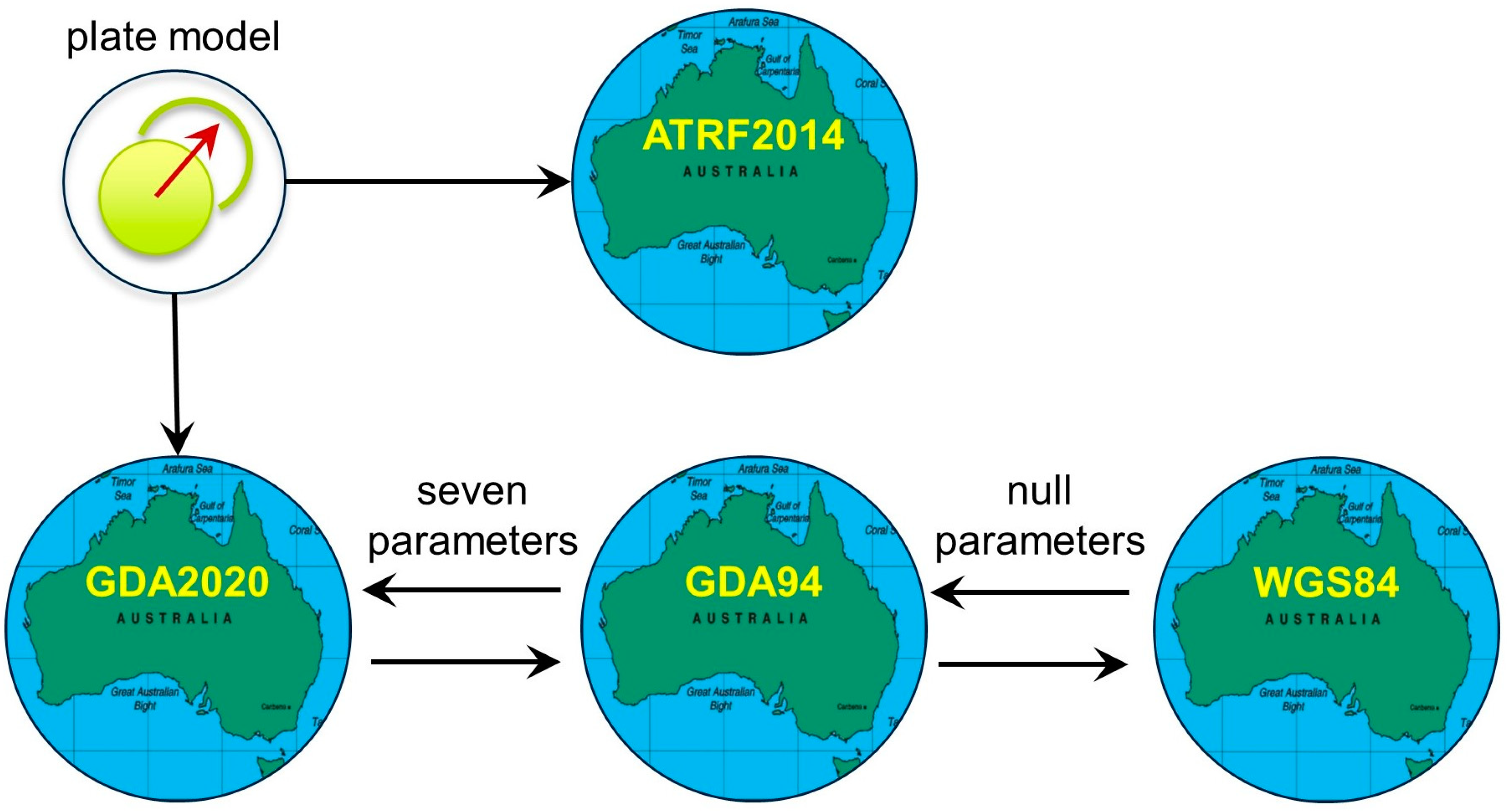
2.2. A Primer on GNSS Datums

Location data collected across a site over time could be referenced to a local reference point or datum. Such data would be internally consistent, avoiding the need to consider continental drift, but would not allow for the import of external datasets based on other data.

The different GNSS positioning systems use different ‘datums’, i.e., GPS WGS84 (World Geodetic System 1984), GLONASS PZ-90, Galileo GTRF, and the BeiDou Coordinate System (BDC). These datums provide an ‘absolute’ (also referred to as ‘dynamic’, ‘time dependent’, or ‘earth-centric’) position of any point on Earth’s surface. In these datums, a given measurement will appear to shift on a map with time due to continental drift. In practice, these data do not continuously accommodate continental plate movement, but provide yearly step changes (benchmarking to ground control point positions on the 1st of July each year). These reference frames are based on an estimate of Earth’s center of mass, a reference ellipsoid used to represent the shape of the Earth, and a geoid, which is the equipotential surface of the Earth’s gravity field and is estimated using an earth gravitational model. The geoid is used to determine the height/elevation of a given point on the surface of the Earth and is generally expressed as elevation relative to mean sea level (MSL). The various data differ in their accuracy of fit to Earth’s surface; they are optimized in terms of representing the whole globe or a part of the globe. Transformation parameters are used for the transformation of coordinates between different reference frames. There are, however, several versions (‘realizations’) of each of these reference frames, and attention to the realization in use is important for sub-meter spatial measurements.

An international consortium has maintained the International Terrestrial Reference System (ITRS) since 1991. The ITRS consists of procedures for creating reference frames, such as a series of implementations of this system, known as the International Terrestrial Reference Frames (ITRFs), the latest of which is ITRF2020. Navigation systems, as used by the various GNSS, are generally referenced to an ITRF solution.

For example, the latest update of the GLONASS reference system was in December 2013 (PZ-90.11) [18]. The transformation from PZ-90.11 to ITRF2008 involves only a shift, without rotation or scale. The Galileo navigation system utilizes the Galileo Terrestrial Reference Frame, which is aligned to new ITRF realizations, with (2σ) differences of less than 3 cm [19]. The China Terrestrial Reference Frame (CGCS) 2000 is referred to as ITRF97 with the epoch of 2000.0.

As the foundation system, the WGS84 coordinate system is widely used. WGS84 was implemented in 1987 with six successive refinements, each using more accurate coordinates of the reference stations. However, Kelly et al. [20] note the changes in WG84 are ‘not well known in the geospatial community’, with many users failing to record which realization data have been captured in WGS84 (G1762), introduced in October 2013, which was reported to have an accuracy (1σ) of 0.5 cm relative to ITRF2008. The latest WGS84 realization, G2139 (released on 3 January 2021), aligned with ITRF2020. The difference between WGS84 and ITRF realizations is mainly due to the use of a different set of base stations by the two systems [20,21].

If the WGS84 realization used in data capture is not recorded, the data are said to be captured in the ‘WGS ensemble’. If the date of data collection is not recorded, no correction can be made for tectonic motion, which is required for a comparison of the measurements made in other years. Geosciences Australia reports the accuracy of the WGS84 ensemble to be between 2–5 m in Australia [22], with uncertainty to increase with time given tectonic movement.

For applications requiring higher accuracy, it is critical that the WGS84 realization epoch and date of data capture (‘coordinate epoch’) be recorded as metadata (Appendix B) to allow for correct transformation to other coordinate systems. The metadata for the transformed dataset should also record the transformation method and parameters used. This ensures other users of the data are aware of the accuracy and lineage of the data. Epochs are recorded as year and decimal year, e.g., 1 January 2020 is 2020.000. Unfortunately, recording formats such as XML or JSON do not provide for such metadata. ISO19115, which defines the schema required for an enhanced description of the acquisition and processing of geographic information, including images [23,24], should be updated to accommodate such a requirement.

The geodetic datum used in China (GCJ-02) is based on WGS-84 but with the use of an obfuscation algorithm that adds random offsets to both the latitude and longitude. A GCJ-02 map will correctly display the location of a point with GCJ-02 coordinates, but a WGS-84 marker will be randomly offset between 100 and 700 m from the expected location on a GCJ-02 map. As required by Chinese law, there is no official API for conversion between GCJ-02 and WGS-84 [25].

As an alternative to the use of a global reference frame, such as WGS84 or ITRF, a local reference frame can be used to provide a better model of the shape of Earth’s surface in a portion of the globe. For example, Australia has implemented the Australian Terrestrial Reference Frame 2014 (ATRF2014) as a dynamic local datum. National data are often mandated for use in activities, such as national mapping and cadastral surveying.

However, ‘static’ objects are changing in global position due to continental drift. Australia is the world’s fastest-moving continent, drifting to the northeast at approximately 7 cm per year, with a much smaller intercontinental movement [26]. Thus, the position of a feature such as an orchard boundary will have shifted by approximately 2 m in 30 years. For operational convenience, location data can be reported in terms of position at a set date using a ‘static’ (also known as ‘time independent’ or ‘plate centric’) datum. For example, Australia operated on the Geocentric Datum of Australia 1994, or GDA94 (with epoch 1999.000), until 2017, when GDA2020 became available [27]. GDA2020 represents locations on the Australian continent as of 2020.000, using the ITRF 2014 at epoch 2020.000.

Thus, high-resolution GNSS measurements are made in terms of a global reference frame, such as WGS84 (G1762), but the data can be presented in a product, e.g., for use in FMIS, in the national geodetic datum. In Australia, both the static datum of GDA2020 and the dynamic datum of ATRF are recognized by the Australian National Measurement Act as standards for measurement of position [28]. Australia supports both dynamic and static data (ATRF and GDA2020, respectively) to cater to the needs of both plate- and global-centric users. A number of countries for which continent drift is not as great an issue have implemented only a local and not a static datum [21].

The parameters for transformation between a given pair of reference frames, e.g., realizations of GDA94, GDA2020, ARTF2014, and WGS84, are described by an ‘EPSG’ number [29] (Figure 1). There are over 6000 EPSG parameter sets, reflecting the myriad of reference frames used globally [30]. The use of an inappropriate transformation in moving between reference frames will introduce spatial error.

For example, if a position reported in a static datum, such as GDA94, is transformed to a dynamic datum, such as WGS84, the point will be represented by its position in the dynamic datum as of 1994.000, unless an additional correction for the date of data collection and continental shift is made (as shown in Figure 1 for the transformation from GDA2020 to ITRF2014). In another example, data captured on WGS 84 with a handheld receiver on 25 April 2023 is likely to have been observed using the latest WGS 84 revision and should be labeled with the coordinate epoch (date of data collection) as WGS 84 (G1762)@2023.315. However, if an augmentation service (RTK, PPP) has been used, it is likely that the data will have been collected in another datum, even though the system software may indicate the use of WGS84. For example, the Australian CORS RTK outputs data in the GDA2020 datum. Transformation of these data to the latest realization of WGS84 will produce WGS 84 (G1762)@2020.000.

For emphasis, geolocation data should be reported in terms of the reference datum and any transformation methods used for data records requiring sub-meter resolution. If a dynamic datum is used, the date of data capture (coordinate epoch) should also be recorded. Further, the uncertainty resulting from the transformation of data should be documented for applications requiring <1 m accuracy [31].

2.3. A Primer on Web Mapping

Veenendaal et al. [32] reviewed trends in web mapping. Briefly, the use of web map services provides an ‘easy’ path for the introduction of a mapping capability within a given service, which is supported by easily available training resources, e.g., Beeflamb [33]. ESRI reports a trend for clients to deliver data to customers using WebGIS (such as ArcGIS Online, arcgis.com accessed on 30 September 2023) rather than by the supply of datasets or production of PDFs, providing ‘live data in the hands of field operators’ [34]. This trend is also true for FMIS, e.g., Zhang et al. [35] discuss design principles for the integration of Google Maps into FMIS. Example applications include the use of Google Maps to visualize locations of tens of thousands of small gardens [36] and locations of animal ‘exploitation farms’ [37]. In non-agricultural examples, GE imagery was used in the display of meteorological satellite data [38], bird species distribution [39], and geochemical data [12]. However, web mapping has several limitations that should be understood in the context of use with FMIS.

The default coordinate system for geolocation data is geographic (longitude and latitude, generally in WGS84), measured in degrees for a given earth model. This geographic data are projected for visualization, e.g., for the display of data in FMIS as a two-dimensional view of Earth’s surface. This process involves a conversion of geographic data to projected coordinates for a given map type and datum. The commonly used Mercator projection involves a cylindrical projection, distorting the pole regions (such that Greenland appears larger than Africa).

A variant of the Mercator projection system that is used in web mapping applications has the official identifier of EPSG:3857 and is known as Web Mercator, ESRI Web Mercator, Google Web Mercator, Spherical Mercator, WGS 84 Web Mercator, and WGS 84/Pseudo-Mercator. The Web Mercator achieved prominence when it was adopted by Google Maps in 2005. Its advantage lies in the use of a spherical (a sphere with a radius of 6,378,137.0 m is assumed) over an ellipsoidal model for the Earth, which requires simpler calculations for the projection of points and thus lower computing resources. However, Web Mercator is not a recognized geodetic system due to the error involved in the projection of latitudes and longitudes from the WGS84 ellipsoid onto a sphere [40]. Distances and angles should not be estimated from Web Mercator maps. Battersby et al. [40] provide details on the implications of using Web Mercator in various online map services.

The most common standards used in serving pre-rendered or on-the-fly computed map tiles over the internet are the Web Map Service (WMS) and the Web Map Tile Service (WTMS) protocols. The OpenLayers library [41] is a commonly used open-source JavaScript library for interfacing web map services in web applications. OpenLayers requires input of data in WGS84 datum by default [42]. To display data on a web mapping application, the typical workflow involves (i) the transformation of data to WGS84, (ii) the transformation of WGS84 data to the Web Mercator (spherical) projection, and (iii) the display of a map.

A number of widely available web map services with global coverage layers are available, including Google Maps, ESRI, Mapbox, Bing Maps, AppleMaps, OpenStreetMap, and Mapquest. Goodchild et al. [43] reviewed the technical specifications of Google Earth, while Lesiv et al. [44] reported on the spatial and temporal availability of imagery in Google Earth and Bing Maps. As mentioned earlier, Chinese web map service providers are required to use obfuscated GCJ02 [25]. The popular provider Beiduo Maps adds a further obfuscation to GCJ-02, termed BD-09, to prevent competitors from accessing Beiduo’s data [45].

The Google Maps service is particularly popular, including in scientific and technical applications [46] due to its availability at higher resolutions (to 15 cm where aerial imagery has been used) and relatively higher currency (imaging dates). The image scale and regularity of image updating of these resources varies by location and is related to population density. Satellite-based imagery is typically used, although input from other platforms is used, e.g., aerial imagery, when available, e.g., from local national mapping agencies [44]. When higher resolution imagery is not available, Landsat imagery (spatial resolution of 15 m) is used [47]. Under their fair use policy, Google Earth (GE) imagery is free for use for websites with less than a certain number of tiles/visits per day.

Local map resources may also be available. For example, the Queensland Government maintains Queensland imagery as an online map service [48]. The resource contains imagery collected on multiple dates from 1930 to 2019 and is a mosaic of ortho-rectified aerial imagery of high spatial resolution (0.5–50 cm) from remotely piloted aircraft, piloted aircraft, and satellites [48]. UAV imagery can also be locally acquired [5,49].

2.4. Positional Accuracy of Web Imagery

Web mapping thus provides an easy-to-use display of geographic information but not a precise geographic information system (GIS). Data collected using the standard WGS84 ellipsoid model is converted on the fly to the Web Mercator spherical model. There is no error at the equator in this conversion, but error increases at higher latitudes, and points can be offset by up to 43 km near the poles. This ‘georeferencing’ error is significant for high-resolution applications, even in near-equatorial positions. Therefore, Web Mercator is not recommended for use in navigation or relative positioning in official use by United States government agencies [50].

Another source of misalignment between WGS84 coordinates of GE imagery and GNSS survey lies in the registration of remotely sensed images to ground control points (GCP) and the compositing/mosaicking of these images, i.e., ‘georeferencing (horizontal distortion)’ and ‘orthorectification (vertical distortion)’ errors. Web tile images are an ortho-mosaic of images from different data sources and spatiotemporal resolutions. Web map providers rely on the image registration undertaken by the image providers. Ideally, this process involves stretching and warping of the image to achieve registration to ground control points (GCPs), e.g., if the camera view is oblique to the ground. However, the satellite imagery consumed by web map providers, such as GE, will not have been registered to GCPs. For example, the positional accuracy (RMSE) of GeoEye-1 images was documented to be 6.0 m on average, ranging from 2 to 9 m for panchromatic images of seven image sets [51]. Further, the mosaicking of images to produce a single image involves automated routines using feature matching, with the translating, stretching, and rotation of images used to match features. The process is not perfect, with positional errors remaining, particularly at high resolutions. The web map providers do not use mosaic images from different sources but rather ‘composite’ them (without feature matching). The merger of images is often visibly noticeable in web imagery. Positional accuracies (horizontal and vertical) and spatial resolution of web map tile images will, therefore, vary temporally (given image updating) with geographic location [52].

Web imagery providers do not provide information on the photogrammetric accuracy of their maps. Various researchers have reported that the positional accuracy of GE imagery varies by location [52,53,54,55]. In these studies, the position of a number of ‘ground control points’ (GCPs) of known (WGS84) geolocations is compared to the location given for that point on Google Maps. For example, a horizontal positional accuracy (RMSE) of 1.73 m was documented in Khartoum across 16 checkpoints [53], while a horizontal positional accuracy (95% confidence level interval) of close to 1 m was documented in Rome from GE imagery across 41 checkpoints [54], and a horizontal positional accuracy (mean absolute error) of 0.13 m in the south and 2.3 m in the northeast of Montreal, Canada, with an overall RMSE of 1.08 m, was estimated using 10 checkpoints [52]. In Addis Ababa, Ethiopia, Mulu et al. [55] reported horizontal positional accuracy (RMSE) of GE imagery at 4.58 m with an error range of between 0.0125 and 5.0 m between GCPs. The RMSE on checkpoint coordinates from Google Maps and corresponding points on Orthophotos (1:4000 scale) in Thailand was reported as 3.3 m (a minimum error of 0.0 m and a maximum error of 28.6 m) [56].

In these examples, a higher error is not associated with a higher latitude, indicating that the Web Mercator projection is not the primary issue in these cases. It is likely that the results relate to the resolution of the available Google Map and the ability of the user to find a checkpoint on the Google Map. For example, as of 13 April 2023, Google Maps provides satellite imagery with maximum resolution that is similar to both Montreal and Rome but lower for Khartoum.

The uncertainty in positional accuracy due to georeferencing and orthorectification errors can limit the use of web maps. If positional accuracy better than 1.5 m is required in the display of geolocated data on a web map, an empirical correction could be made based on an assessment of the positional accuracy of the GE imagery. For local mapping, a 2D conformation transformation can be used for transformation between grid coordinate systems using a four-parameter transformation (also known as a similarity or Helmert’s transformation) based on the parameters of scale, rotation, and translation in both x and y directions. These four parameters can be estimated when two horizontal control points are known in both Universal Transverse Mercator (UTM) coordinate systems. In this conformal transformation, straight lines remain straight, and orthogonal angles are preserved. This procedure is illustrated in the following case study.

3. Case Study Materials and Methods

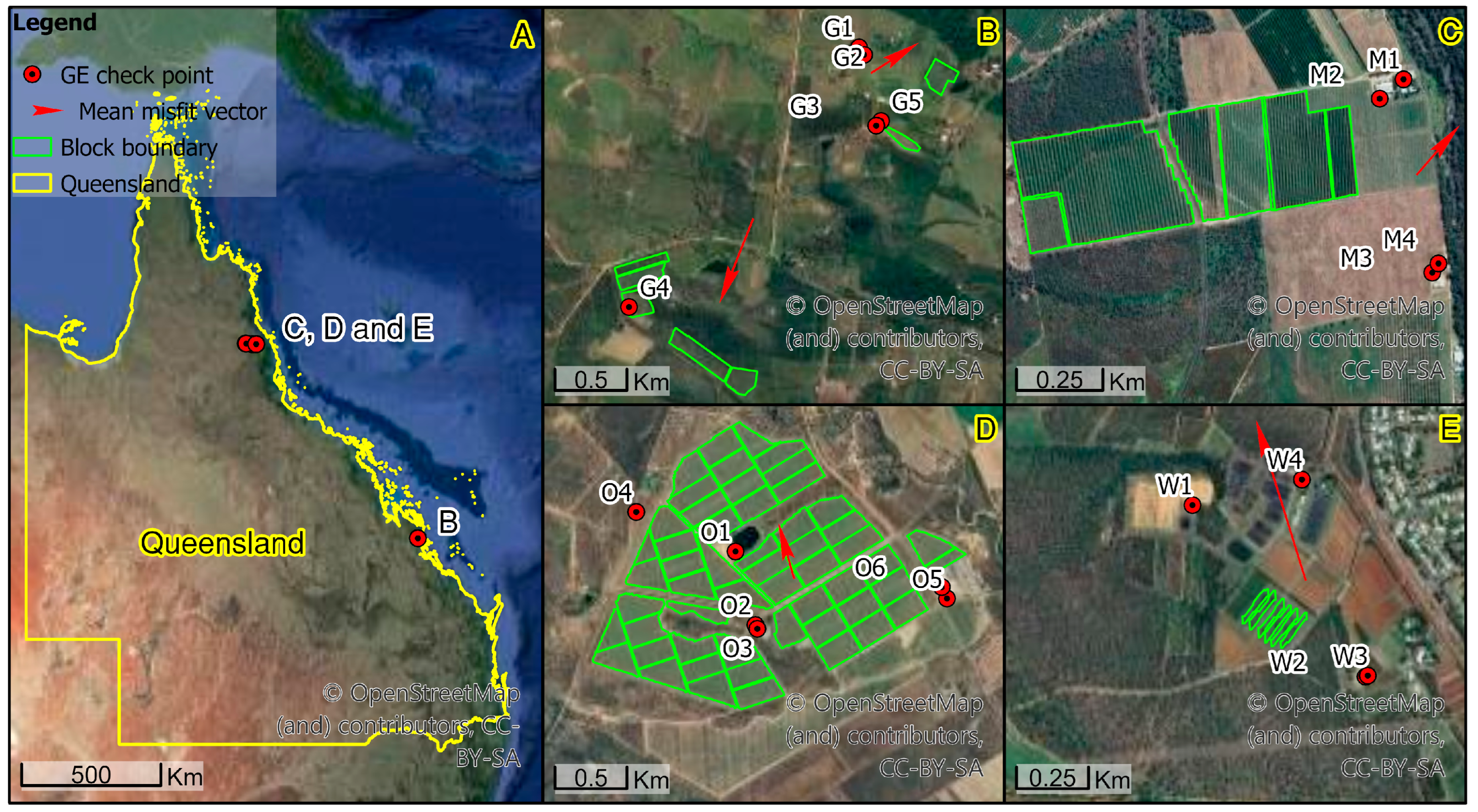
3.1. Study Area

Data were collected from four sites (

Table 1. Site locations (WGS84) in Central Queensland (CQ) and Far North Queensland (FNQ), Australia, with site descriptors and date of the survey.

Farm	Latitude (°)	Longitude (°)	Elevation (m)	Landscape	Survey Date
CQ-1	23.025080	150.641167	50–81	Hilly	24 March 2022
FNQ-1	17.131778	145.303059	499–521	Plain	10 November 2023
FNQ-2	17.112235	145.100360	459–501	Plain	10 November 2023
FNQ-3	17.134072	145.427091	587–591	Plain	10 November 2023

and Figure 2) in Central and Far North Queensland, Australia.

3.2. GNSS Survey and Imagery Data

Site imagery was accessed from Google Earth Pro imagery (at 200 m range, from CNES/Airbus for 2023) [46], Bing [57], ESRI [34], and Queensland imagery [48]. Additionally, an orthoimage was acquired over the Central Queensland site in January 2023 using a UAV. A sub-25 kg multirotor drone equipped with a Sony RGB camera (ILCE-6000) and a 25 mm fixed focal lens was flown at an average height of 110 m altitude, capturing photography with a Ground Sampling Distance (GSD) of about 1.6 cm. Ground Control Points (GCPs) were positioned between the orchard rows at approximately 200 m apart (n = 66 GCPs over 34.5 ha). The GCP locations were fixed with an Altus ASP3 GNSS rover operating with base station positioned at points established by a Leica GS14 GNSS receiving real-time kinematic (RTK) corrections from the CORS network (HxGN Smart Net, C.R. Kennedy, Melbourne, Australia [58]), with location data captured using the MGA94 coordinate system. The orthoimage and Digital Elevation Model (DEM) were generated in Agisoft Metashape (version 1.5.2.7838), providing two- and five-centimeter GSDs, respectively.

A minimum of two checkpoints (ground control) were assessed for each site. These points were chosen as being identifiable in Google Earth Pro imagery and ground verifiable. Coordinates were extracted for points at the intersection of two lines, e.g., the corner of a roof or concrete slab. Line segments were extracted from the image using a line segment detector algorithm deployed in OpenCV [59]. The same process was followed for ESRI, Bing, and Queensland web imageries, for historic GE imagery, and for drone imagery. The historical imagery differed in spatial resolution and source; it was from either Maxar Technologies, CNES, or Airbus.

Field GNSS survey data were captured in WGS84 (GDA2020 epoch) using a GS14 receiver-operated RTK mode through connection to a CORS network for the Central Queensland sites. For Far North Queensland sites, Queensland Government [60] survey control markers (SCMs) close to each farm were located using the application ‘Benchmrk’ [61] and used as ground control points (GCPs) in the transfer of coordinates to the checkpoints.

The difference between GNSS and web imagery coordinates of the checkpoints was calculated for eastings (ΔE) and northings (ΔN) (Equations (1) and (2)) and used in the calculation of a horizontal positional misfit vector (Equation (3)).

$$\Delta E=E_{GEI}-E_{GNSS}$$

(1)

$$\Delta N=N_{GEI}-N_{GNSS}$$

(2)

$$e=\sqrt{\Delta E^2+\Delta N^2}$$

(3)

3.3. Accuracy Assessment and Position Correction

Horizontal accuracy was calculated from the root mean square error statistic on easting (RMSE_x, Equation (4)) and northing (RMSE_y, Equation (5)) measurements for a number of checkpoints (n) on a given farm. Overall accuracy (RMSE_r) was calculated following the American Society for Photogrammetry and Remote Sensing (ASPRS) positional accuracy standard for digital geospatial data [62] (Equation (6)), with a 95% confidence interval on horizontal accuracy calculated as RMSE_r x 1.7308 [63].

$${RMSE}_x=\sqrt{\frac{\sum {\left(E_{GEI}-E_{GNSS}\right)}^2}{n}}$$

(4)

$${RMSE}_y=\sqrt{\frac{\sum {\left(N_{GEI}-N_{GNSS}\right)}^2}{n}}$$

(5)

$${RMSE}_r=\sqrt{{{RMSE}_x}^2+{{RMSE}_y}^2}$$

(6)

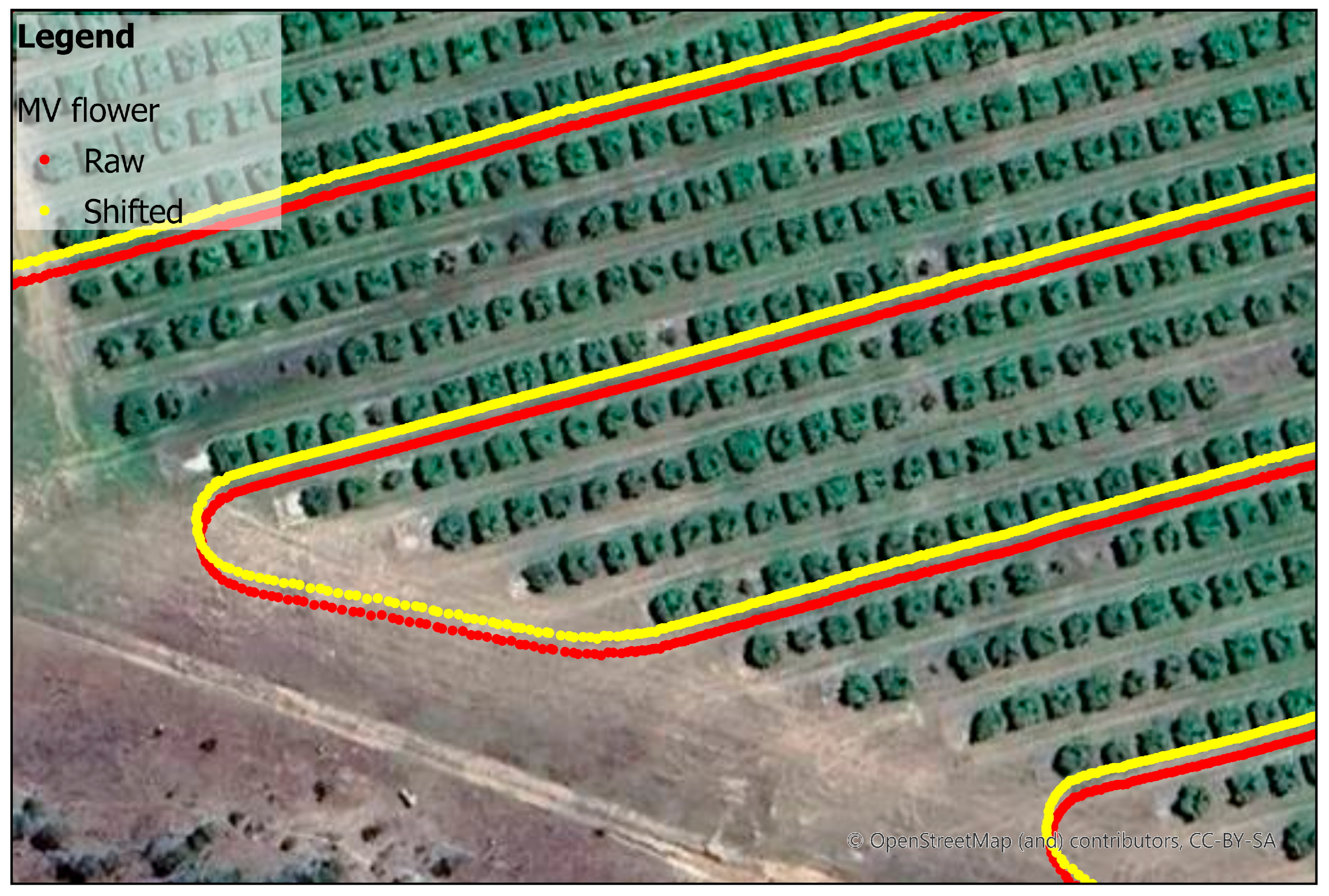
3.4. Adjustment of Misalignment

A 2D conformal transformation was devised to align GNSS data and GEI. If X_GEI represents coordinates in GE imagery and X_GNSS represents observed GNSS coordinates over the checkpoints of a given area, a 2D dimensional similarity transformation [64] can be presented as:

$$X_{GEI}={sRX}_{GNSS}+\Delta X$$

(7)

where s is the scale factor, R is the rotation matrix of the x-axis cosine angle ($\theta$) in a counterclockwise direction, and ΔX is the translational vector. The rotation matrix can be described as:

$$R=\left|\begin{array}{cc}Cos\theta & -Sin\theta \\ Sin\theta & Cos\theta \end{array}\right|$$

(8)

If a = sCosθ and b = sSinθ, the transformation equation can be represented in matrix form as:

$${\left|\begin{array}{c}{E}_i\\ N_i\end{array}\right|}_{GEI}={\left|\begin{array}{cc}{E}_i& {-N}_i\\ N_i& E_i\end{array}\begin{array}{cc}1& 0\\ 0& 1\end{array}\right|}_{GNSS}\left|\begin{array}{c}\begin{array}{c}a\\ b\end{array}\\ \begin{array}{c}\Delta E\\ \Delta N\end{array}\end{array}\right|$$

(9)

where:

$$s=\sqrt{a^2+b^2}$$

(10)

$$\theta ={\tan }^{-1}\frac{b}{a}$$

(11)

In the special case of when the scale factor is unity and there is no rotation, the matrix equation is represented as:

$${\left|\begin{array}{c}{E}_i\\ N_i\end{array}\right|}_{GEI}={\left|\begin{array}{c}{E}_i\\ N_i\end{array}\right|}_{GNSS}+\left|\begin{array}{c}\Delta E\\ \Delta N\end{array}\right|$$

(12)

A 2D conformal transformation may not present a perfect solution for a set of control points. A least squares solution was, therefore, used to compute transformation parameters to minimize error on coordinate pairs.

4. Case Study Results

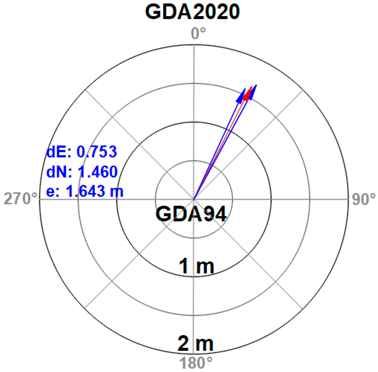
4.1. Tectonic Shift

The mean horizontal shift vector between GDA1994 and GDA2020 positions of the farm GCPs was a vector of 1.643 m in a northeast direction (

Table 2. Estimation of the shift vector between GDA2020 and GDA94 coordinates of survey control marks (SCMs) used as ground control points (GCPs) on each of the five farms.

Farm	SCM	GDA94 Coordinates		GDA20 Coordinates		Misfit Vectors
		Latitude (°)	Longitude (°)	Latitude (°)	Longitude (°)	Magnitude (m)	Bearing (°)
CQ-1	147698	−23.032350	150.629297	−23.032338	150.629304	1.581	25.1876
CQ-2	046749	−23.313954	150.517036	−23.313941	150.517043	1.580	24.9753
FNQ-1	073155	−17.115310	145.283933	−17.115297	145.283940	1.687	28.6620
FNQ-2	140459	−17.132102	145.098745	−17.132088	145.098752	1.687	28.5861
FNQ-3	208477	−17.126252	145.425309	−17.126239	145.425317	1.684	28.7109
Mean misfit vector						1.643	27.2794

and Figure 3), as expected for 25 years of tectonic movement of the Australian plate at approximately 6.5 cm per year [65]. The shift was slightly lower in Central Queensland (CQ) than in Far North Queensland (FNQ) (Table 2).

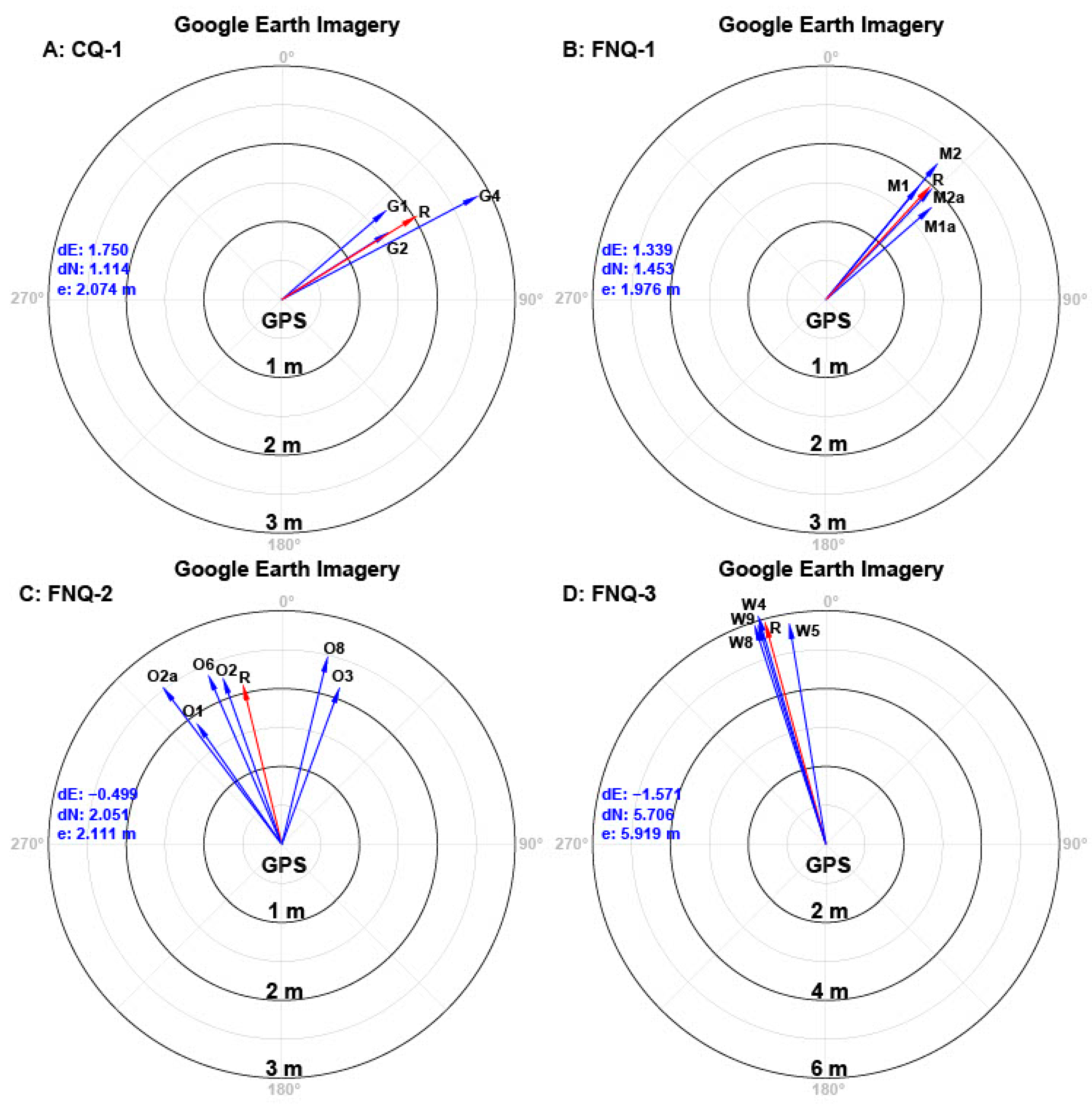
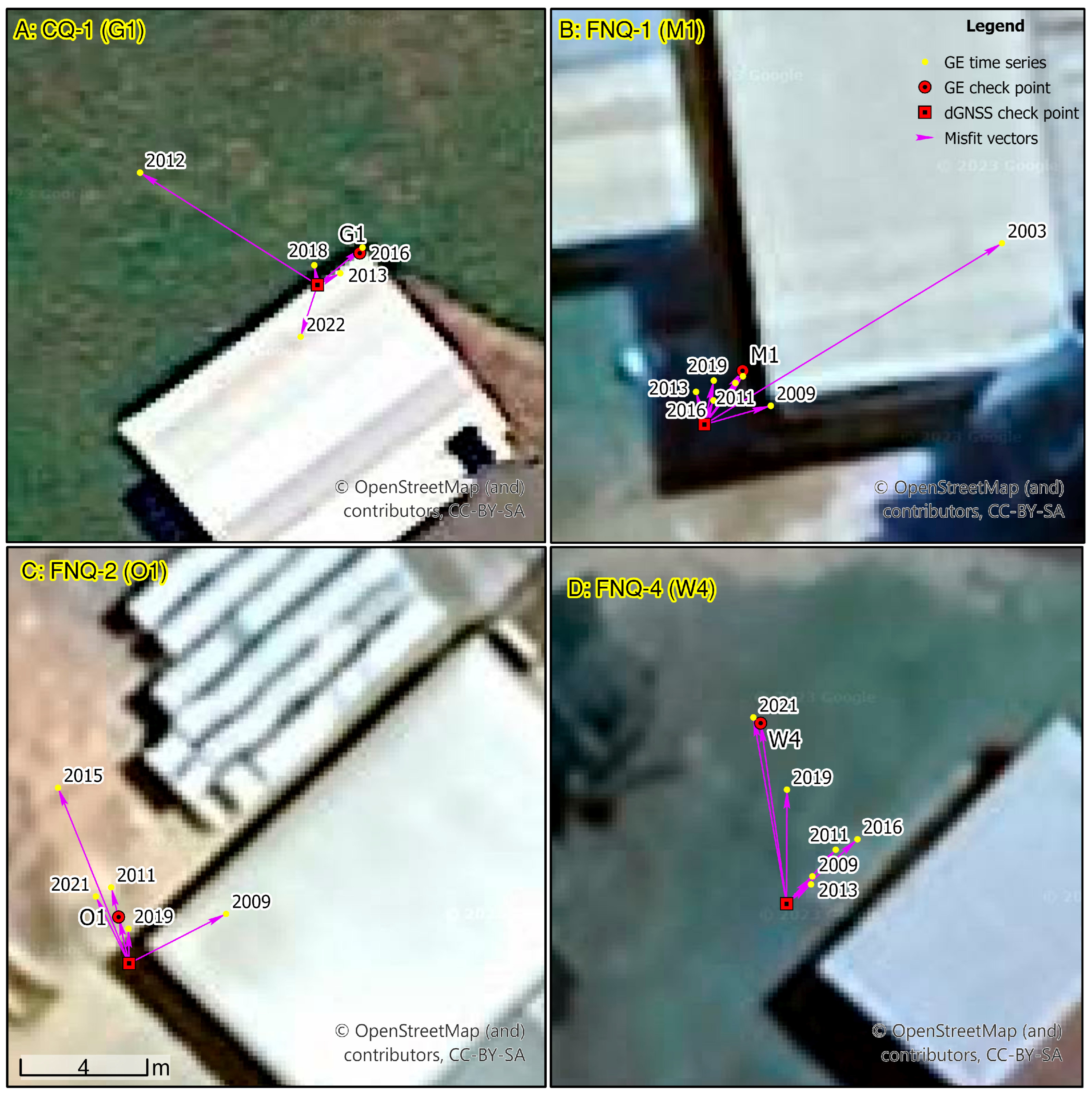
4.2. Current Imagery Misfit Vectors

The positional accuracy of available web imagery is expected to vary within the coverage of a farm, between farms, between historical images, and between images from different web imagery providers. This uncertainty will be due to (a) poor resolution of the web imagery, leading to inaccuracy of location of a given feature in the Web Mercator projection, (b) image registration error inherent in the source of data, (c) the use of the spheroid model in the Web Mercator projection, and (d) tectonic shift. Tectonic shift error is introduced as web imagery is typically recorded in the WGS84@ date of image capture.

The mean misfit vectors were calculated in the WGS84 Universal Transverse Mercator (UTM) coordinate system. The vectors varied between farms and between years of GEI, e.g., varying from 1.976 m to 5.919 m in magnitude and from 42.6576° to 346.3344° on the CQ-1 farm (

Table 3. Observed misfit vectors between GNSS (WGS84 GDA2020 epoch) and Google Earth web imagery coordinates (WGS84@ date of image capture) from 2016 and 2021 and 2022 web imagery.

Farm	CP	GNSS Coordinates		GEI Coordinates		Misfit Vectors
		Latitude (°)	Longitude (°)	Latitude (°)	Longitude (°)	Magnitude (m)	Bearing (°)
CQ-1	G1	−23.019277	150.635479	−23.019268	150.635491	1.768	49.5702
	G2	−23.019747	150.635811	−23.019739	150.635825	1.628	57.9389
	G3	−23.024222	150.636543	−23.024210	150.636568	2.854	62.2218
	Mean misfit vector in 2016					2.074	57.5329
	G4	−23.035339	150.619628	−23.035369	150.619612	3.661	205.1533
	G5	−23.023893	150.636911	−23.023918	150.636902	2.897	197.2232
	Mean misfit vector in 2022					3.271	201.6509
FNQ-1	M1	−17.131629	145.303576	−17.131613	145.303587	1.883	39.4433
	M2	−17.132104	145.302916	−17.132092	145.302924	1.804	48.9154
	M3	−17.136690	145.304139	−17.136673	145.304154	2.263	39.3829
	M4	−17.136450	145.304314	−17.136441	145.304331	1.970	43.7701
	Mean misfit vector in 2021					1.976	42.6576
FNQ-2	O1	−17.109832	145.086829	−17.109819	145.086826	1.897	324.8323
	O2	−17.114471	145.087914	−17.114457	145.087916	2.266	340.4727
	O3	−17.114718	145.088043	−17.114699	145.088031	2.533	322.8433
	O4	−17.107115	145.080498	−17.107099	145.080504	2.146	20.2694
	O5	−17.113312	145.100384	−17.113289	145.100384	2.372	336.5229
	O6	−17.112584	145.100071	−17.112566	145.100081	2.482	13.7519
	Mean misfit vector in 2021					2.111	346.3344
FNQ-3	W4	−17.129009	145.423667	−17.128958	145.423660	5.758	350.5385
	W1	−17.129677	145.420099	−17.129622	145.420084	6.131	343.4351
	W2	−17.135245	145.425488	−17.135193	145.425472	5.928	341.8832
	W3	−17.135216	145.425558	−17.135162	145.425542	5.898	342.7705
	Mean misfit vector in 2021					5.919	344.6045

and Figure 4). The highest variance in misfit vectors of GCPs occurred on the FNQ-2 farm, which was likely associated with the size of this farm (2 km across), and thus had the potential for the presence of several images. The highest magnitude misfit vector was observed on the FNQ-1 farm. An RMSE of 3.432 m, with an RMSEx of 1.391 m and an RMSEy of 3.137 m, was calculated for the difference between GEI and GNSS (WGS84 GDA2020 epoch) for the combined data of all sites.

4.3. Historical Imagery Misfit Vectors

The misfit vector of one prominent CP per farm was calculated using historical GE imagery (2003 to 2022) for a given farm. Misfit vectors at a given site varied in both magnitude and direction (

Table 4. GE coordinates (WGS84@ imagery date) of farm checkpoints (CPs) and their misfit vectors relative to GNSS measurements. Checkpoint (CP) codes relate to those in Table 3.

Farm/CP	Imagery Date	GEI Coordinates		Misfit Vectors
		Latitude (°)	Longitude (°)	Magnitude (m)	Bearing (°)
CQ-1/G1	2 August 2012	−23.019245	150.635429	6.178747	303.3369
	5 August 2013	−23.019274	150.635485	0.784156	65.3325
	13 May 2016	−23.019266	150.635492	1.767559	49.5702
	19 January 2018	−23.019271	150.635478	0.569779	354.9467
	11 February 2022	−23.019292	150.635474	1.733135	193.8136
	Mean misfit vector			1.036	316.4531
FNQ-1/M1	15 July 2003	−17.131577	145.303660	10.633708	237.1640
	10 July 2009	−17.131623	145.303595	2.089216	253.0876
	18 June 2011	−17.131617	145.303585	1.603096	215.3983
	28 June 2013	−17.131619	145.303574	1.057875	165.7280
	25 September 2016	−17.131622	145.303578	0.806052	199.0387
	14 July 2019	−17.131616	145.303579	1.408654	190.9744
	10 April 2021	−17.131615	145.303587	1.909719	217.0331
	Mean misfit vector			2.593	227.0259
FNQ-2/O1	10 July 2009	−17.109818	145.086856	3.317411	241.4570
	19 August 2011	−17.109811	145.086824	2.445809	166.6781
	15 September 2015	−17.109782	145.086809	5.909510	158.1297
	14 July 2019	−17.109822	145.086829	1.087267	178.4557
	15 June 2021	−17.109813	145.086819	2.329465	153.7840
	Mean misfit vector			2.532	175.8819
FNQ-3/W4	8 December 2009	−17.129002	145.423675	1.158942	221.7447
	18 June 2011	−17.128994	145.423681	2.242521	220.8642
	28 June 2013	−17.129004	145.423674	0.952090	230.1685
	25 September 2016	−17.128991	145.423688	2.937458	226.3162
	14 July 2019	−17.128977	145.423668	3.568632	179.7362
	18 July 2021	−17.128957	145.423658	5.915459	169.8191
	Mean misfit vector			2.523	195.4489

and Figure 5), with a minimum of 0.56 m and a maximum of 10.6 m. Old imagery generally had greater errors than more recent imagery, but the highest error for the FNQ-3 site (5.9 m) was associated with the most recent image (2021).

4.4. Misfit Vectors by Imagery Source

Misfit vectors were also calculated for web imageries other than GE imagery using the same GCPs (

Table 5. Misfit vectors for the images of four sites from four web imagery providers (doa 15/4/2023).

Farm/CP	Misfit Vectors in Web Imagery
	Bing		Google		ESRI		QLD Globe
	Magnitude (m)	Bearing (°)	Magnitude (m)	Bearing (°)	Magnitude (m)	Bearing (°)	Magnitude (m)	Bearing (°)
CQ-1/G1	5.712	225.053691	1.768	49.570205	1.141	251.483588	0.429	69.585256
FNQ-1/M1	2.357	218.344693	1.883	219.443312	4.218	261.485087	1.919	190.089089
FNQ-2/O1	4.049	268.553544	1.897	144.832330	2.596	290.962091	4.306	114.349462
FNQ-3/W4	4.774	164.826241	5.758	170.538496	1.918	306.876470	1.024	161.457136
Mean	3.365	218.086680	1.963	163.813842	2.319	276.766311	1.556	136.118854

). The highest errors were associated with the Bing web imagery and the lowest with the Queensland imagery (Table 5 and

Table 6. Average RMSE across the four sites for four web imagery providers.

Imagery	RMSEx (m)	RSMEy (m)	RMSExy (m)
Bing	3.018	3.199	4.398
Google	1.155	3.086	3.295
ESRI	2.588	0.823	2.716
QLD	1.985	1.386	2.421

). By way of comparison, the misfit vector estimated for the drone imagery collected at CQ-1/G1 was 0.016 m and bearing 0.123574° (the average across eight GCPs).

In comparison, the horizontal and vertical positional accuracies achieved for the drone imagery were 0.0127 and 0.0029 m, respectively. A similar result was reported with the use of a moderate number of GCPs by Gómez-Candón et al. [5], who reported a spatial resolution of 7.4, 14.8, and 24.7 mm and an accuracy of 1.5, 2.6, and 2.5 (±1.2) mm for UAV mosaiced images collected at flying altitudes of 30, 60, and 100 m, respectively, using a 12.3 MP Olympus EP-1 camera.

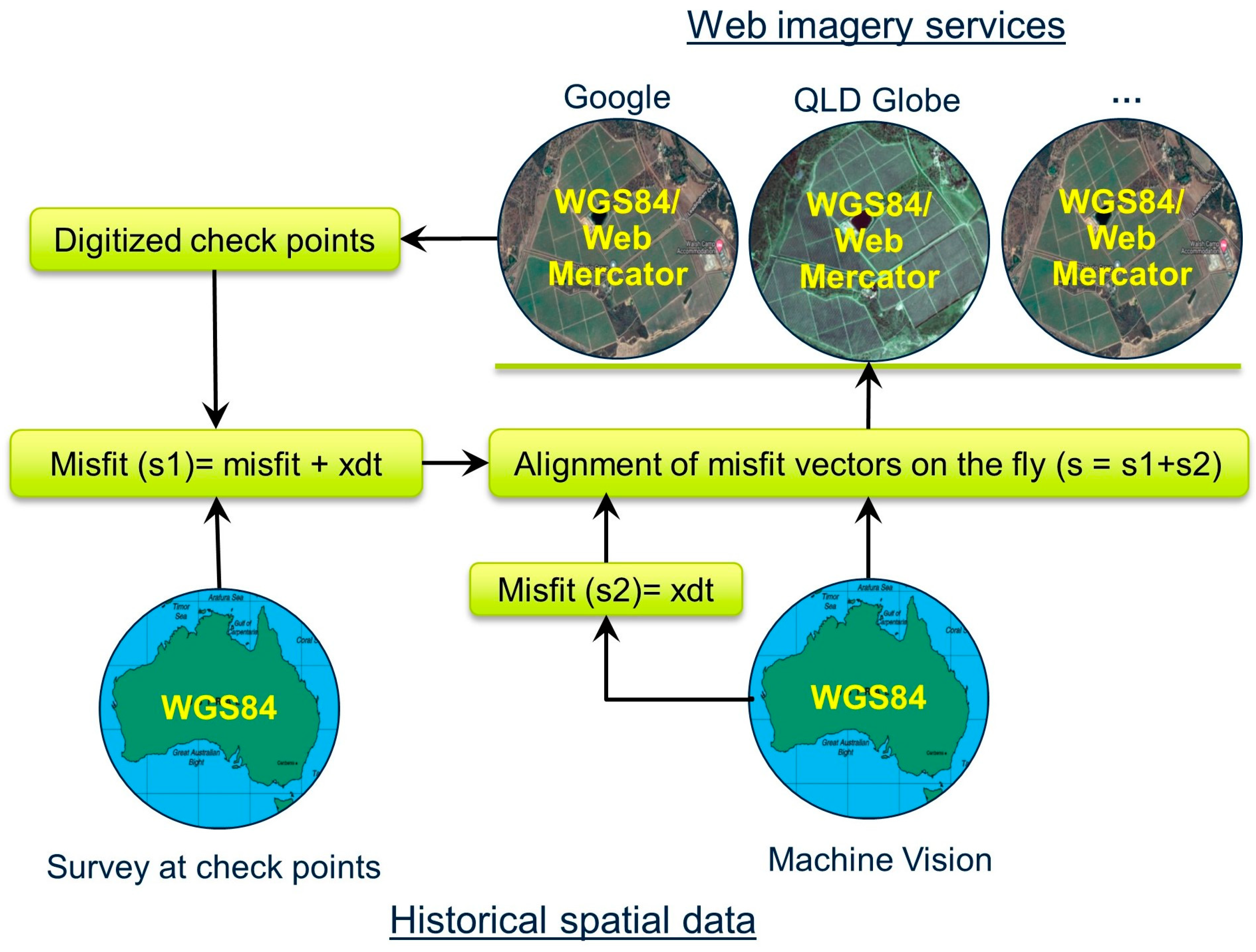
4.5. Misfit Adjustment for Web Mapping

The least squared approximation method for 2D conformal transformation was used in the estimation of four transformational parameters to align GNSS data with GE web imagery. For all sites, the scale factor was unity, and the rotational value was near zero (with average values of s: 0.9999 and $\theta$: 0.0273). A simple mean shift vector is, therefore, recommended to translate GNSS data for display on GE web imagery. For example, for the FNQ-2 orchard (with row-to-row spacing of 8 m), a shift of −0.499 m east and 2.051 m north was applied for the alignment of GNSS data acquired on 21 August 2022 from a moving vehicle with 2021 GE web imagery (Figure 6).

The web mapping error could, therefore, be empirically accommodated through the following workflow (Figure 7):

• Establishment

  (i)

  Identify probable checkpoints in web imagery;

  (ii)

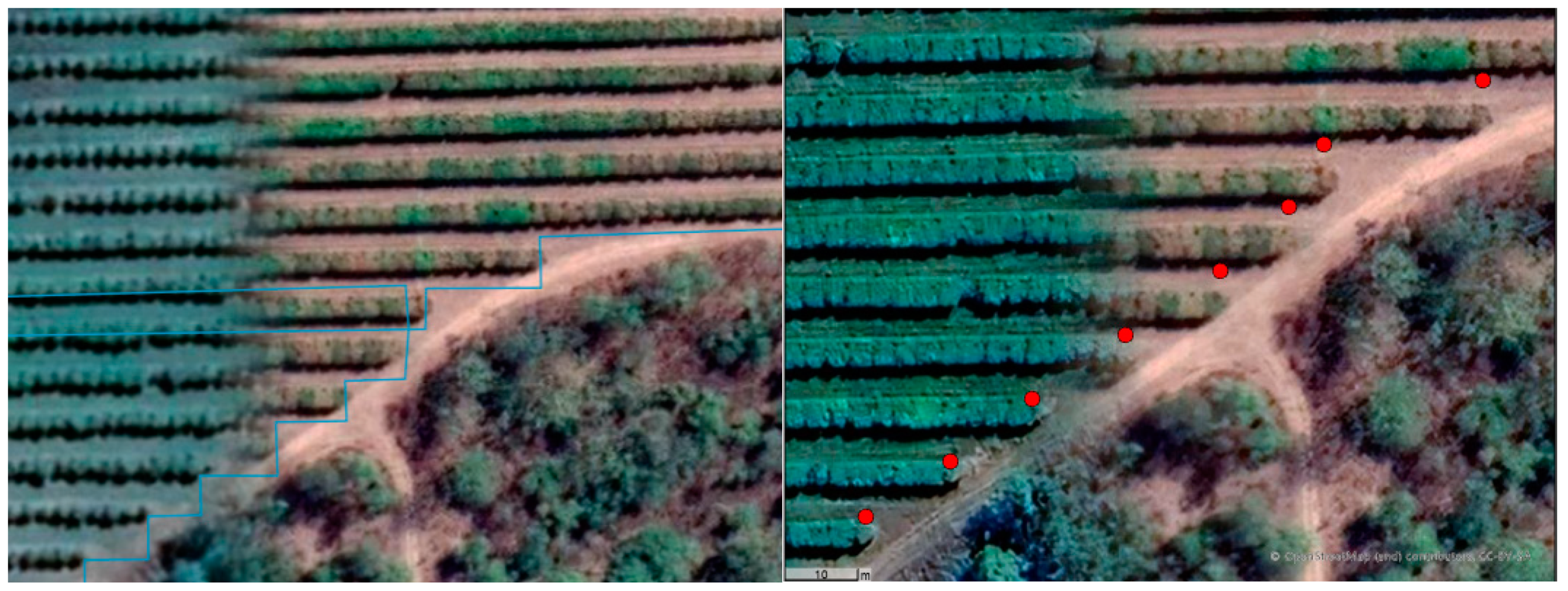
  Extract coordinates of these points using line segment intersection points;

  (iii)

  Acquire GCP location data using WGS84 (GDA2020 epoch) datum, GDA2020, or ATRF2014, or an equivalent national system;

  (iv)

  Estimate the misfit vector(s) from web imagery with respect to CPs (s1 = misfit + xdt) and plate model (s2 = xdt), where x is the magnitude of plate movement over the time interval (dt) between coordinate epoch and 2020.000 (of CP or MV) data;

  (v)

  Curate the misfit vector for each farm, each web imagery provider, and each date of the image.

• Implementation

  (i)

  Collect and curate field data with the metadata of the datum and the date of acquisition;

  (ii)

  For web map display, convert data to WGS84 (with GDA2020 epoch);

  (iii)

  Apply the misfit vector to all field-collected data ‘on-the-fly’ before display;

  (iv)

  Undertake client-side transformation WGS84 to Web Mercator datum by the web mapping application.

However, this approach is invalidated when different imageries are present for one farm at a given time from a web map provider, as shown in the example in Figure 8. In this example (right panel), the misfit of the position of end trees of each tree row is between 2019 and 2022 GE web imageries.

5. Discussion

Imagery is useful for the operationalization of FMIS, for the location of farm features, e.g., orchard boundaries, and for the visualization of spatial data. The use of publicly available web mapping resources, such as GE, is driven by the convenience of the availability of these resources. Given this convenience, the use of such resources is expected to increase. However, these resources are compromised in applications that require sub-meter spatial resolutions. In the case study of the current study, the average RMSE on GCP positions was 5.930 and 3.432 m for within-farm and between-farm data, respectively; for the most recent (2023) GE web imagery, 4.334 m across historical (post-2015) GE web images of one farm and 3.036 m between the most recent images from four web imagery service providers.

There are several sources of error in the records of location data to FMIS: (a) survey measurement, (b) tectonic shift, and (c) mapping. Survey error depends on the methodology and technology used, e.g., standalone, dGNSS, or RTK. Errors are also introduced due to the use of the WGS84 ensemble dynamic datum, which ignores the tectonic shift. The misfit vector due to the tectonic shift (at approx. 6.5 cm/year for the Australian plate) can be ignored for measurements spanning a few years but not for longer periods in applications requiring sub-meter level accuracy. This misfit will vary with location but is well modeled and thus can be corrected.

Map errors include problems with image registration and rectification, as well as errors involved in the compositing/mosaicking of images, i.e., ‘georeferencing (horizontal distortion)’ and ‘orthorectification (vertical distortion)’, image processing and mapping, and the earth model employed. For example, GNSS data are collected using an ellipsoidal earth model, but data are converted on the fly to the web Mercator spheroid earth model for display on web maps. Another type of map error is associated with the spatial resolution of the image. The positional errors or misfit vectors were calculated based on the availability. The resolution of publicly available web imageries assessed in this study varied spatially and temporally. For example, GE web imagery from Maxar Technologies in Central Queensland (2016) has a pixel dimension of 0.15 m, while CNES/Airbus in Far North Queensland (2021) was 0.30 m. Higher image spatial resolutions are associated with higher location accuracies of GCPs and thus image registrations.

The publicly available web map services are thus impressive for their global coverage and image currency but suffer significant positional accuracy issues in the context of farm management applications.

6. Conclusions

The impact of continental drift on location measurements on a farm across time can be addressed by the use of a local datum., i.e., a local reference position. However, the likely availability of mass-market RTK/PPP devices, driven by the availability of services, such as Ginan (in Australia), and the increasing ubiquity of farm connectivity, driven by the availability of services, such as Starlink, should drive the use of the national official static datum. For example, the national static datum is GDA2020 in Australia and ETRS89 in Europe. Another advantage of using the local official datum is compatibility for access to government-curated data layers, e.g., road networks.

Applications requiring high spatial accuracy should avoid the use of publicly available web maps through the use of alternate imagery, e.g., georeferenced aerial (UAV) imagery can be collected for the farm. This solution adds cost in the form of drone imaging but it decreases operational complexity by avoiding the need for ongoing corrections.

The geodetic field is in a state of flux as the availability and use of high spatial resolution data increases. Users providing applications targeted to farm operations, e.g., autonomous vehicles using GNSS, should be aware of likely changes. To support the accurate use of collected data, it is essential to record the date of data capture and the coordinate reference station and system used, including the realization of WGS84 if employed, and any transformations undertaken. There is a pressing need to update metadata recording within data formats, such as JSON, to capture data for the documentation of datum and coordinates systems used in data capture, processing, storage/management, and delivery, with attendant location error estimation. Failure to document such metadata provides the user with an illusion of accuracy and compromises the future use of quality data.

References

1. Li, X.; Barriot, J.-P.; Lou, Y.; Zhang, W.; Li, P.; Shi, C. Towards Millimeter-Level Accuracy in GNSS-Based Space Geodesy: A Review of Error Budget for GNSS Precise Point Positioning. Surv. Geophys. 2023, 44, 1–90. [Google Scholar] [CrossRef]
2. Realini, E.; Caldera, S.; Pertusini, L.; Sampietro, D. Precise GNSS positioning using smart devices. Sensors 2017, 17, 2434. [Google Scholar] [CrossRef] [PubMed]
3. Fontana, R.; Latterman, D. GPS Modernization and the Future. In Proceedings of the IAIN World Congress and the 56th Annual Meeting of The Institute of Navigation, San Diego, CA, USA, 26–28 June 2000. [Google Scholar]
4. Controlled Traffic Farming. What Is Controlled Traffic Farming? 2023. Available online: https://www.actfa.net/controlled-traffic-farming/ (accessed on 12 April 2023).
5. Gómez-Candón, D.; De Castro, A.; López-Granados, F. Assessing the accuracy of mosaics from unmanned aerial vehicle (UAV) imagery for precision agriculture purposes in wheat. Precis. Agric. 2014, 15, 44–56. [Google Scholar] [CrossRef]
6. Anderson, N.T.; Walsh, K.B.; Koirala, A.; Wang, Z.; Amaral, M.H.; Dickinson, G.R.; Sinha, P.; Robson, A.J. Estimation of Fruit Load in Australian Mango Orchards Using Machine Vision. Agronomy 2021, 11, 1711. [Google Scholar] [CrossRef]
7. Jabir, B.; Falih, N.; Rahmani, K. Accuracy and efficiency comparison of object detection open-source models. Int. J. Online Biomed. Eng. 2021, 17, 165. [Google Scholar] [CrossRef]
8. Dorman, M. Introduction to Web Mapping, 1st ed.; Chapman and Hall/CRC: Boca Raton, FL, USA, 2020; p. 366. [Google Scholar]
9. Tsiropoulos, Z.; Fountas, S. Farm management information system for fruit orchards. In Precision Agriculture’15; Wageningen Academic Publishers: Wageningen, The Netherlands, 2015; pp. 44–55. [Google Scholar]
10. Jones, V.P.; Brunner, J.F.; Grove, G.G.; Petit, B.; Tangren, G.V.; Jones, W.E. A web-based decision support system to enhance IPM programs in Washington tree fruit. Pest Manag. Sci. Former. Pestic. Sci. 2010, 66, 587–595. [Google Scholar] [CrossRef] [PubMed]
11. Forcén-Muñoz, M.; Pavón-Pulido, N.; López-Riquelme, J.A.; Temnani-Rajjaf, A.; Berríos, P.; Morais, R.; Pérez-Pastor, A. Irriman platform: Enhancing farming sustainability through cloud computing techniques for irrigation management. Sensors 2021, 22, 228. [Google Scholar] [CrossRef]
12. Zuo, R.; Yin, B. Google Earth-aided visualization and interpretation of geochemical survey data. Geochem. Explor. Environ. Anal. 2022, 22, 2. [Google Scholar] [CrossRef]
13. Baselga, S.; Olsen, M.J. Approximations, errors, and misconceptions in the use of map projections. Math. Probl. Eng. 2021, 2021, 1094602. [Google Scholar] [CrossRef]
14. USA, GPS Accuracy. 2023. Available online: https://www.gps.gov/systems/gps/performance/accuracy/ (accessed on 12 April 2023).
15. Catapult. Demystifying Sample Rate in Satellite-Based Athlete Tracking Technologies. 2023. Available online: https://www.catapultsports.com/blog/sample-rate-satellite-athlete-tracking-technologies (accessed on 17 April 2023).
16. Claughton, D.; Coon, A. Inmarsat I-4F1 Satellite Outage Disables Tractor GPS Services for Farming Operations and Some Maritime Safety. 2023. Available online: https://www.abc.net.au/news/rural/2023-04-18/inmarsat-i-4f1-satelite-outage-asia-pacific-gps-farms/102234678 (accessed on 24 April 2023).
17. Ginan. Ginan: GNSS Analysis Centre Software. 2023. Available online: https://www.ga.gov.au/scientific-topics/positioning-navigation/positioning-australia/about-the-program/analysis-centre-software (accessed on 24 April 2023).
18. Zueva, A.; Novikov, E.; Pleshakov, D.; Gusev, I. System of Geodetic parameters. In Proceedings of the 9th Meeting of the International Committee on GNSS (ICG-9), Prague, Czech Republic, 10–14 November 2014; Available online: https://www.unoosa.org/pdf/icg/2014/icg-9/icg-9-jointstatement.pdf (accessed on 2 October 2023).
19. Gendt, G.; Altamimi, Z.; Dach, R.; Söhne, W.; Springer, T.; Team, T.G.P. GGSP: Realisation and maintenance of the Galileo terrestrial reference frame. Adv. Space Res. 2011, 47, 174–185. [Google Scholar] [CrossRef]
20. Kelly, K.M.; Dennis, M.L. Transforming between WGS84 realizations. J. Surv. Eng. 2022, 148, 04021031. [Google Scholar] [CrossRef]
21. Donnelly, N.; Crook, C.; Haasdyk, J.; Harrison, C.; Rizos, C.; Roberts, C.; Stanaway, R. Dynamic datum transformations in Australia and New Zealand. Proc. Res. Locate 2014, 14, 48–59. [Google Scholar]
22. Geoscience Australia. WGS84. 2023. Available online: https://www.ga.gov.au/scientific-topics/positioning-navigation/wgs84 (accessed on 20 March 2023).
23. ISO 19115-2:2019(en); Geographic Information—Metadata—Part 2: Extensions for Acquisition and Processing. OBP: Geneva, Switzerland, 2023. Available online: https://www.iso.org/obp/ui/#iso:std:iso:19115:-2:ed-2:v1:en (accessed on 2 May 2023).
24. AS/NZS ISO 19115.2:2019; Geographic Information—Metadata—Part 2: Extensions for Acquisition and Processing. Standards New Zealand: Wellington, New Zealand, 2023. Available online: https://www.standards.govt.nz/shop/asnzs-iso-19115-22019/ (accessed on 2 May 2023).
25. GCJ-02. GCJ-02 Explained: The Chinese Coordinate System—For Developers. 2023. Available online: https://hackernoon.com/why-mapbox-was-the-best-tech-partner-for-my-chinese-coordinate-system-development-azo737mo (accessed on 24 April 2023).
26. ATRF. Australian Terrestrial Reference Frame. 2023. Available online: https://www.icsm.gov.au/australian-terrestrial-reference-frame (accessed on 24 April 2023).
27. ICSM. Geocentric Datum of Australia 2020. 2023. Available online: https://www.icsm.gov.au/gda2020 (accessed on 20 April 2023).
28. Federal Register of Legislation. National Measurement Act 1960—Recognized-Value Standard of Measurement of Position 2012 (No. 1). 2023. Available online: https://www.legislation.gov.au/Details/F2012L00800 (accessed on 20 April 2023).
29. Featherstone, W.E. An updated explanation of the geocentric datum of Australia (GDA) and its effects upon future mapping. Aust. Surv. 1996, 41, 121–130. [Google Scholar] [CrossRef]
30. Maptiler. EPSG.io: Find Coordinate Systems Worldwide. 2023. Available online: https://epsg.io/about (accessed on 5 May 2023).
31. Haasdyk, J.; Janssen, V. The many paths to a common ground: A comparison of transformations between GDA94 and ITRF. In Proceedings of the International Global Navigation Satellite Systems Society, IGNSS Symposium, University of New South Wales. Sydney, NSW, Australia, 15–17 November 2011. [Google Scholar]
32. Veenendaal, B.; Brovelli, M.A.; Li, S. Review of web mapping: Eras, trends and directions. ISPRS Int. J. Geo-Inf. 2017, 6, 317. [Google Scholar] [CrossRef]
33. Beeflamb. User Guide: Use Google My Maps to Map Your Farm. 2023. Available online: https://beeflambnz.com/knowledge-hub/PDF/use-google-my-maps-map-your-farm.pdf (accessed on 4 May 2023).
34. ESRI. Esri Australia Technical Blog. 2023. Available online: https://esriaustraliatechblog.wordpress.com/tag/gda2020/ (accessed on 2 May 2023).
35. Zhang, M.; Mei, J. The design and implementation of electronic farm system based on Google Maps. In Proceedings of the 2010 Third International Symposium on Intelligent Information Technology and Security Informatics, Jian, China, 2–4 April 2010. [Google Scholar]
36. Hu, S.; Dai, T. Online map application development using Google Maps API, SQL database, and ASP.NET. Int. J. Inf. Commun. Technol. Res. 2013, 3, 102–110. [Google Scholar]
37. Barnes, A.; White, R. Mapping emotions: Exploring the impact of the Aussie Farms Map. J. Contemp. Crim. Justice 2020, 36, 303–326. [Google Scholar] [CrossRef]
38. Chen, A.; Leptoukh, G.; Kempler, S.; Lynnes, C.; Savtchenko, A.; Nadeau, D.; Farley, J. Visualization of A-Train vertical profiles using Google Earth. Comput. Geosci. 2009, 35, 419–427. [Google Scholar] [CrossRef]
39. Benham, P.M.; Beckman, E.J.; DuBay, S.G.; Flores, L.M.; Johnson, A.B.; Lelevier, M.J.; Schmitt, C.J.; Wright, N.A.; Witt, C.C. Satellite imagery reveals new critical habitat for endangered bird species in the high Andes of Peru. Endanger. Species Res. 2011, 13, 145–157. [Google Scholar] [CrossRef]
40. Battersby, S.E.; Finn, M.P.; Usery, E.L.; Yamamoto, K.H. Implications of web Mercator and its use in online mapping. Cartogr. Int. J. Geogr. Inf. Geovis. 2014, 49, 85–101. [Google Scholar] [CrossRef]
41. Schmidt, C. OpenLayers: Free Maps for the Web. 2023. Available online: http://www.openlayers.org/ (accessed on 7 August 2023).
42. Haklay, M.; Weber, P. Openstreetmap: User-generated street maps. IEEE Pervasive Comput. 2008, 7, 12–18. [Google Scholar] [CrossRef]
43. Goodchild, M.F.; Guo, H.; Annoni, A.; Bian, L.; De Bie, K.; Campbell, F.; Craglia, M.; Ehlers, M.; Van Genderen, J.; Jackson, D. Next-generation digital earth. Proc. Natl. Acad. Sci. USA 2012, 109, 11088–11094. [Google Scholar] [CrossRef] [PubMed]
44. Lesiv, M.; See, L.; Laso Bayas, J.C.; Sturn, T.; Schepaschenko, D.; Karner, M.; Moorthy, I.; McCallum, I.; Fritz, S. Characterizing the spatial and temporal availability of very high resolution satellite imagery in google earth and microsoft bing maps as a source of reference data. Land 2018, 7, 118. [Google Scholar] [CrossRef]
45. Dmistry, S. A Short Guide to the Chinese Coordinate System. GCJ-02(gcj 02) Explained. 2023. Available online: https://abstractkitchen.com/blog/a-short-guide-to-chinese-coordinate-system/ (accessed on 4 May 2023).
46. Yu, L.; Gong, P. Google Earth as a virtual globe tool for Earth science applications at the global scale: Progress and perspectives. Int. J. Remote Sens. 2012, 33, 3966–3986. [Google Scholar] [CrossRef]
47. Potere, D. Horizontal positional accuracy of Google Earth’s high-resolution imagery archive. Sensors 2008, 8, 7973–7981. [Google Scholar] [CrossRef]
48. State of Queensland. Queensland Imagery: Latest State Program. 2023. Available online: https://spatial-img.information.qld.gov.au:443/arcgis/rest/services/Basemaps/LatestStateProgram_AllUsers/ImageServer (accessed on 4 April 2023).
49. Zhang, C.; Valente, J.; Kooistra, L.; Guo, L.; Wang, W. Opportunities of UAVs in orchard management. Int. Arch. Photogramm. Remote Sens. Spat. Inf. Sci. 2019, 42, 673–680. [Google Scholar] [CrossRef]
50. NGA (National Geospatial-Intelligence Agency). NGA standardization document, Map Projections for GEOINT Content, Products, and Applications National Center for Geospatial Intelligence Standards: 3838 Vogel Road, Arnold. 2017. Available online: https://earth-info.nga.mil/php/download.php?file=coord-mapproj (accessed on 2 October 2023).
51. Gómez-Candón, D.; López-Granados, F.; Caballero-Novella, J.J.; Pena-Barragán, J.M.; García-Torres, L. Understanding the errors in input prescription maps based on high spatial resolution remote sensing images. Precis. Agric. 2012, 13, 581–593. [Google Scholar] [CrossRef]
52. Goudarzi, M.A.; Landry, R.J. Assessing horizontal positional accuracy of Google Earth imagery in the city of Montreal, Canada. Geod. Cartogr. 2017, 43, 56–65. [Google Scholar] [CrossRef]
53. Mohammed, N.Z.; Ghazi, A.; Mustafa, H.E. Positional accuracy testing of Google Earth. Int. J. Multidiscip. Sci. Eng. 2013, 4, 6–9. [Google Scholar]
54. Pulighe, G.; Baiocchi, V.; Lupia, F. Horizontal accuracy assessment of very high resolution Google Earth images in the city of Rome, Italy. Int. J. Digit. Earth 2016, 9, 342–362. [Google Scholar] [CrossRef]
55. Mulu, Y.A.; Derib, S.D. Positional Accuracy Evaluation of Google Earth in Addis Ababa, Ethiopia. Artif. Satell. 2019, 54, 43–56. [Google Scholar] [CrossRef]
56. Methakullachat, D.; Witchayangkoon, B. Coordinates comparison of Goolge® Maps and orthophoto maps in Thailand. Int. Trans. J. Eng. Manag. Appl. Sci. Technol. 2019, 10, 1–8. [Google Scholar]
57. Pendleton, C. The world according to Bing. IEEE Comput. Graph. Appl. 2010, 30, 15–17. [Google Scholar] [CrossRef]
58. HxGN SmartNet Aus. 2023. Available online: https://hxgnsmartnet.com/en-au/services/customer-login (accessed on 12 April 2023).
59. Von Gioi, R.G.; Jakubowicz, J.; Morel, J.-M.; Randall, G. LSD: A line segment detector. Image Process. On Line 2012, 2, 35–55. [Google Scholar] [CrossRef]
60. Queensland Government. Survey Control Mark Report. 2023. Available online: http://qspatial.information.qld.gov.au (accessed on 22 March 2023).
61. Benchmrk. The Most Accurate Locations in Australia. 2023. Available online: https://geolocarta.com/benchmrk (accessed on 13 April 2023).
62. ASPRS. ASPRS positional accuracy standards for digital geospatial data. Photogramm. Eng. Remote Sens. 2015, 81, A1–A26. [Google Scholar] [CrossRef]
63. FGDC. Geospatial Positioning Accuracy Standards Part 3: National Standard for Spatial Data Accuracy; National Aeronautics and Space Administration: Virginia, NV, USA, 1998.
64. Kraus, K. Photogrammetry: Geometry from Images and Laser Scans; Walter de Gruyter: Berlin, Germany, 2007; Volume 1. [Google Scholar]
65. Janssen, V. GDA2020, AUSGeoid2020 and ATRF: An introduction. In Proceedings of the Association of Public Authority Surveyors Conference (APAS2017), Shoal Bay, Australia, 20–22 March 2017. [Google Scholar]
Figure 1. Coordinate transformation between GDA2020, GDA94, ATRF, and WGS84. Note that transformations from the ensemble WGS84 will introduce a ca. 5 m uncertainty to the data.
Agronomy 13 02563 g001
Figure 2. The location of the mango orchards overlaid with GE web imagery with the farm-block boundaries in green and checkpoints in red circles with a black center spot. (A) Location of farms in Far North and Central Queensland. (BE) Image farms CQ-1, FNQ-1, FNQ-2, and FNQ-3, respectively. The red arrows are the mean misfit vectors observed for the checkpoints on each farm. Arrow length represents 2.075 and 3.271 m in B for 2016 and 2022, respectively, and 1.976, 2.111, and 5.919 m for (B), (C), (D), and (E), respectively, for 2021 imagery.
Agronomy 13 02563 g002
Figure 3. Observed horizontal positional shift vectors between GDA94 and GDA2020 for GCPs on five farms (blue arrows) and the mean shift vectors (red arrow).
Agronomy 13 02563 g003
Figure 4. Representation of horizontal positional misfit vectors (in WGS84 UTM) between GNSS (coordinate epoch 1/2023 displayed in a GDA2020 epoch) and GE (2016 in CQ-1 and 2021 in FNQs) coordinates of ground control points on four farms: ((A) CQ-1, (B) FNQ-1, (C) FNQ-2, and (D) FNQ-3). Blue and red arrows are individual and mean misfit vectors, respectively.
Agronomy 13 02563 g004
Figure 5. Misfit vectors calculated from the GNSS GDA2020 assessed the location of the GCP and Google Earth images over five years at four farm sites. Vectors are displayed in 2016 for the Google Earth image for (A) and the 2021 image for (B), (C), and (D), respectively.
Agronomy 13 02563 g005
Figure 6. Display of GNSS data from a moving vehicle on FNQ-2 on 21 August 2022 on 2021 GE web imagery. The red points are raw GNSS WGS84 (GDA2020 epoch) data collected at 10 Hz. The yellow points are adjusted using a misfit shift vector of −0.499 m east and 2.051 m north, estimated from GCPs on the farm.
Agronomy 13 02563 g006
Figure 7. Workflow for the misfit adjustment for web mapping.
Agronomy 13 02563 g007
Figure 8. Example of GE web imagery for a mango orchard (latitude: −12.7380033, longitude: 131.1731937). Left panel doa 5 July 2023; right panel doa 8 July 2023. In both cases, the imagery has two data sources, with the right side of both images sourced from Maxar, July 2022, and the left side of the images from CNES/Airbus, April 2019 (left panel), and Airbus, May 2022 (right panel). Red dots on the right panel represent the position of the crown center of the end trees of each row in GE (CNES/Airbus) imagery from April 2019.
Agronomy 13 02563 g008