Article

STICS Soil–Crop Model Performance for Predicting Biomass and Nitrogen Status of Spring Barley Cropped for 31 Years in a Gleysolic Soil from Northeastern Quebec (Canada)

1
Department of Soils and Agri-Food Engineering, Laval University, Paul Comtois Bldg, Quebec City, QC G1V 0A6, Canada
2
Doctoral School “Sciences and Environment” (ED 304), University of Bordeaux, 33405 Talence, France
3
Quebec Research and Development Centre, Agriculture and Agri-Food Canada, 2560 Hochelaga Blvd, Quebec City, QC G1V 2J3, Canada
4
INRAE, Bordeaux Science Agro, UMR 1391 ISPA, F-33140 Villenave-d’Ornon Cedex, France
5
Quebec Research and Development Centre, Agriculture and Agri-Food Canada, 1468 St-Cyrille Street, Normandin, QC G8M 4K3, Canada
*
Author to whom correspondence should be addressed.
Agronomy 2023, 13(10), 2540; https://doi.org/10.3390/agronomy13102540
Submission received: 12 September 2023 / Revised: 27 September 2023 / Accepted: 28 September 2023 / Published: 30 September 2023
(This article belongs to the Topic Advances in Crop Simulation Modelling)

Abstract

:
Spring barley (Hordeum vulgare L.) is an increasingly important cash crop in the province of Quebec (Canada). Soil–crop models are powerful tools for analyzing and supporting sustainable crop production. STICS model has not yet been tested for spring barley grown over several decades. This study was conducted to calibrate and evaluate the STICS model, without annual reinitialization, for predicting aboveground biomass and N nutrition attributes at harvest during 31 years of successive cropping of spring barley grown in soil (silty clay, Humic Gleysol) from the Saguenay–Lac-Saint-Jean region (northeastern Quebec, Canada). There is a good agreement between observed and predicted variables during the 31 successive barley cropping years. STICS predicted well biomass accumulation and plant N content with a low relative bias (|normalized mean error| = 0–13%) and small prediction error (normalized root mean square error = 6–25%). Overall, the STICS outputs reproduced the same trends as the field-observed data with various tillage systems and N sources. Predictions of crop attributes were more accurate in years with rainfall close to the long-term average. These ‘newly calibrated’ parameters in STICS for spring barley cropped under continental cold and humid climates require validation using independent observation datasets from other sites.

1. Introduction

Spring barley (Hordeum vulgare L.) is used as cattle feed and for malting but grain barley production remains insufficient to meet the demand in the province of Quebec (Canada) [1]. Even with the use of high-performance cultivars and improved crop management over the last decades, grain barley yields remain lower than in western Europe [2,3]. Average annual barley grain yields in Canada were 2.0 Mg DM ha−1 between 1960 and 1989, and 2.7 Mg DM ha−1 between 1990 and 2021 [4] compared to about 4.4 Mg DM ha−1 for western Europe [5].
The cold and humid continental climate of eastern regions of Canada, including the province of Quebec, poses significant constraints for crop production [6]. About 52% of the barley acreage in the province of Quebec is located in areas with limiting soil and climate conditions such as the Bas-Saint-Laurent, Gaspésie, Îles-de-la-Madeleine and Saguenay–Lac-Saint-Jean [1]. In these areas, the mean annual temperature ranges from 1 to 3 °C, and the last spring frost occurs late, up to the end of May. The sum of growing degree days (GDD, basis 0 °C) between April and October ranges from 1800 to 2200 °C d, which corresponds to severe to moderate limitations for spring-sown small grains according to climatic suitability ratings [7]. Moreover, soils with excess water and poor fertility also limit crop production in these areas [8]. For barley, waterlogging can reduce yields by 20 to 85% depending on the duration and intensity of the waterlogging at different stages of the plant’s development and the cultivar tolerance [9].
The short growing season in several regions of northeastern Quebec dictates the choice of cultivars that can be grown successfully. Cultivars are known to differ in their phyllochron, which is positively correlated with temperature and daylength [10]. Phenological traits were also shown to vary with locations [11]. For instance, the time needed to reach anthesis from sowing is about 55 days (860–940 °C d) for two spring barley cultivars, Cadette (a semidwarf lodging-resistant type) and Leger (a standard lodging-susceptible type) grown under climatic conditions of Montreal region (province of Quebec) [12], but 10–20 days longer (up to 1200 °C d) in western Europe [12,13]. Differences in cultivars and length of the growing season between western Europe and northeastern Quebec should therefore be taken into account in process-based models of barley growth and development. Understanding the growth and development of barley cultivars adapted to the cold and humid conditions of northeastern Quebec, which has a short growing season is crucial for improving cultivars and crop management practices.
Soil–crop models are valuable and powerful tools for understanding many complex processes in agroecosystems [14]. They can be used to predict and analyze crop growth attributes [15] and the use of nitrogen (N) [16,17] and water [18,19]; to assess the environmental impacts of agriculture by taking into account crop management, soils, and climate [20,21,22]; and to test longer-term scenarios in the context of global warming [23,24]. Several soil–crop models have been developed that differ in their structure, simulated process and approach [25], scales (plant, field, watershed, or regional) [26], and objectives [27]. A number of process-based soil–crop models (e.g., DAISY, DSSAT-CERES, HERMES, MONICA, and WOFOST) are available for spring barley crops grown in Europe [17,28]. In western Canada, Jame et al. [29] developed a crop model using DSSAT for wheat and barley grown on the Great Plains of the Canadian province of Alberta. STICS (Simulateur mulTIdisciplinaire pour les Cultures Standard) is a generic soil–crop model initially developed in France for wheat (Triticum turgidum L. subsp. durum) and maize (Zea mays L.) and then for other annual and perennial crops in Europe [30,31]. STICS simulates crop growth and development along with soil water, C, and N processes [23,32]. It has been tested in a large number of soil–plant agroecosystems and was designed to adapt easily to various crops and diverse climatic conditions [33,34,35]. STICS was tested and validated for spring barley cultivars cropped in the temperate climate of western Europe [32,36].
In Canada, STICS was calibrated and validated for soybean (Glycine max L. Merr) and spring wheat (Triticum aestivum L.) cultivars cropped in several sites distributed between southwestern Quebec province and southern Ontario province, which highlighted the opportunities for using STICS in areas with a short growing season [37]. The integration of a snow-cover module has extended the possibility of using STICS for cold and humid continental regions [38]. STICS has also been calibrated and evaluated for non-consecutive simulations with annual resetting under these conditions for maize [39], potato (Solanum tuberosum L.) [40], and timothy (Phleum pratense L.) [41].
No crop growth model has been yet calibrated and evaluated over long-term cropping periods without annual resetting for spring barley in the soil and climate conditions of the Saguenay–Lac-Saint-Jean region (northeastern Quebec, Canada). This region occupies an immense territory (106.5 million km2) relatively far from the rest of the province of Quebec [42] and constitutes the northern limit of the practice of agriculture in Quebec. Its 149,204 hectares of soil with agricultural potential [43] and the combination of the cool climate and isolated geographic location provide the region with a unique place in the agricultural industry due to its geographical position within the boreal zone. The objectives of this study were (i) to statistically analyze a dataset of dry matter aboveground biomass, grain yield, grain and shoot N concentration and N uptake at harvest over 31 successive cropping years of spring barley cultivars selected for the pedoclimatic conditions of the Saguenay–Lac-Saint-Jean region; (ii) to calibrate and evaluate the ability of STICS to predict the above-mentioned variables over several decades without annual reinitialization; and (iii) to compare the two approaches: Are STICS predictions for the experimental site and the associated database better or not than a statistical model?

2. Materials and Methods

2.1. Experimental Site and Field Database

The study was conducted using a long-term experiment that was initiated in the fall of 1989, at the Agriculture and Agri-Food Canada’s Normandin Experimental Farm, at Normandin city, located in the regional county municipality of Maria-Chapdelaine, in the Saguenay–Lac-Saint-Jean region of the Canadian province of Quebec (lat. 48°50′ N; long. 72°33′ W; alt. 137 m). Since 1936, research conducted there has significantly helped to improve farming practices in Quebec’s Saguenay—Lac-Saint-Jean region [44]. The region has a cold and humid continental climate. For the 31 years considered in this study, cumulative rainfall from 10 days before seeding date to grain harvest ranged from 176 to 498 mm with an average of 317 mm. The average temperature was 16.0 °C (14.3–18.4 °C), the sum of GDD above 0 °C ranged from 1431 to 1775 °C d, and the cumulative global radiation ranged from 1543 to 2259 MJ m−2. Values for each of the 31 years are presented in Table S1 for the growing season and the entire year. The soil is a Labarre series silty clay (Humic Gleysol). Soil characteristics are presented in Table 1. The site had been cultivated under a spring barley–alfalfa (Medicago sativa L.) rotation for about 10 years prior to 1990.
The experimental design was a factorial split-split-plot replicated four times with two types of crop rotation randomized into main plots (a continuous barley in monoculture and a 3-year cereal-perennial forage rotation), two tillage systems randomly assigned to subplots and two N sources randomly assigned to sub-subplots [45]. Only the plots cropped with continuous barley in monoculture (16 plot units 10 m × 5 m in size) were considered in this study. Six-row spring barley cultivars Chapais (1990–2014) and Alyssa (2015–2020) [46], both having similar ecophysiological parameters, were sown between 9 and 31 May at a rate of 360 grains m−2 using a conventional cereal seeder. Details of the N application along with dates of seeding, harvest, and tillage for each year are provided in Table S2. The two tillage systems consisted of a moldboard plow operated to a 20 cm depth (MP) and a chisel plow to a 15 cm depth (CP), with tillage performed yearly in the fall after harvest. The two N sources were ammonium nitrate (MIN) and N-based liquid dairy manure (LDM), applied according to local recommendations. The LDM were analyzed annually, and N concentrations were determined using a LECO CNS-1000 analyzer (LECO Corp., St. Joseph, MI, USA). Before seeding, plots under the MIN treatment received 70 kg N ha−1yr−1 as ammonium nitrate, 17.5 kg P ha−1yr−1 as triple superphosphate, and 58 kg K ha−1yr−1 as potassium chloride. For the LDM plots, about 50 m3 ha−1yr−1 of liquid dairy manure obtained from a local farm was applied in early spring, providing an average of 107 ± 24 kg total N ha−1yr−1, 17 ± 4 kg total P ha−1yr−1, and 119 ± 29 kg total K ha−1yr−1. Annual amounts of N applied as LDM from 1990 to 2020 are reported in Table S2.

2.2. Plant Analysis

Grain yield (GY) and straw yield were determined every year from 1990 to 2020 in the 16 experimental plots. Grain and straw yields were measured in an 8.2 m × 1.62 m area at grain maturity between mid-August and mid-September depending on the year (Table S2), using a Wintersteiger plot harvester (Salt Lake City, UT, USA). Dry matter content of grain and straw was determined on a fresh 500 g subsample after drying in a forced draft oven at 55 °C to constant weight. Straw residues were returned to the soil after harvest. Nitrogen concentrations in grain (NCG) and straw were measured only from 1997 to 2020. Dried and ground (to pass through a 1 mm screen) subsamples of grain and straw were digested using a mixture of sulfuric and selenious acids, as described by Isaac and Johnson [47]. The N concentration in digested solutions was measured by automated colorimetry using a Lachat QuikChem 8000 autoanalyzer (QuikChem Method 13-107-06-2-E; Lachat Instruments, Milwaukee, WI, USA). Dry matter aboveground biomass (grain + straw) (AGB), N concentration in AGB (NCAGB), and N accumulation in AGB (NU) and grain (NAG) were then calculated.

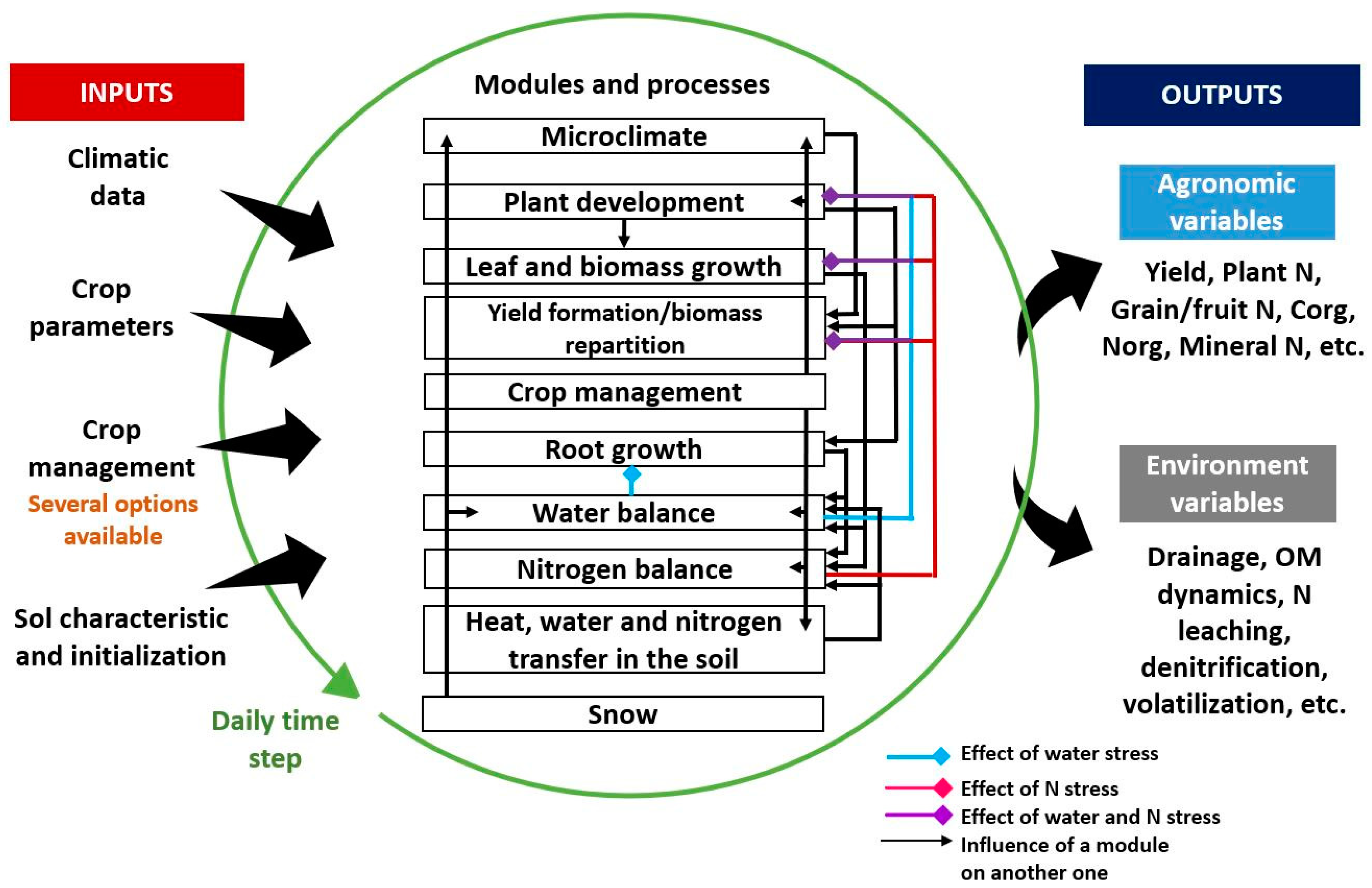
2.3. STICS Soil–Crop Model Overview

STICS is a generic soil–crop model applicable to a wide variety of agroecosystems which has been in development since 1996 [30,31,48]. Based on general ecophysiological concepts and soil processes that describe the functioning of soil–plant systems, STICS simulates the dynamic of soil–crop systems on a daily time step as a function of climatic conditions, crop and soil characteristics, and management practices (Figure 1). It calculates agricultural (e.g., crop yield and grain N content) and environmental (e.g., soil water and mineral N contents, N leaching, and soil organic carbon dynamic) variables simultaneously [23]. STICS has several interdependent modules and sub-modules which were built by assembling and synthesizing parts or formalisms of existing models [48,49]. Each module or sub-module deals with a particular physical or ecophysiological process, and variables are exchanged between modules and sub-modules. The description of these processes mostly relies on a unique set of general parameters. In STICS, two types of plant parameters are defined: cultivar parameters and generic parameters that are assumed to be the same for all cultivars of the same species. An in-depth description of STICS concepts, mathematical equations, general parameterization, and uses can be found in Brisson et al. [49] and Beaudoin et al. [48].
Briefly, the phenological development stages of a given crop cultivar, are expressed in development units that are mainly governed by thermal (degree day), photothermal, or vernal-photothermal indices (according to the species) but are also affected by limiting factors such as soil water and N content. Shoot biomass accumulation is calculated from the leaf area index (LAI) by converting intercepted radiation into biomass using the radiation use efficiency (RUE) concept. These processes are closely influenced by the phenological development stage, temperature, and plant density along with water stress and N stress. The grain C content is derived from the retranslocation of vegetative C as well as from the continued assimilation of C during grain filling. The GY is calculated by applying a progressive “harvest index” to the AGB dry weight of the plant [48], i.e., the ratio of the biomass accumulated in the GY from the beginning of grain filling until maturity is an increasing proportion of the AGB.
Plant N accumulation depends on soil mineral N availability in the soil–root system (and symbiotic fixation for legumes) and on crop N requirements. Crop N requirements were calculated using the concept of maximum (Ncmax) and critical N (Nc) dilution curves. The Ncmax curve represents the plant’s maximum capacity to accumulate N in its shoot biomass and is used in STICS to calculate potential crop N uptake. The Nc curve represents the N concentration in shoots required to produce the maximum AGB at a given time [50]. It can be used to calculate the N nutrition index (NNI), which is the ratio of the actual N concentration to Nc. The NNI is used to determine if the plant is under N stress or not. An NNI below 1 will reduce potential crop growth. For spring barley, the Ncmax and Nc were calculated using the following equations: Ncmax = 6.66 × (Shoot Biomass)−0.39 and Nc = 4.76 × (Shoot Biomass)−0.39, respectively [51]. As with C, NAG is calculated as a function of a dynamic N harvest index, i.e., the amount of N accumulated in grains from the beginning of grain filling until maturity is an increasing proportion of the amount of N in the AGB.
In STICS, the soil is described as a succession of up to five horizontal layers with their hydrodynamic and pedological characteristics. Soil-dependent modules calculate water, C, and N balances and, consequently, the effects of water stress and N stress on crops. Humus mineralization depends on soil characteristics (clay and CaCO3 content), soil organic N content, temperature, and soil water content. Mineralization of organic residues is calculated as a function of the C/N ratio based on the model of Nicolardot et al. [52]. Interactions between soil and crops occur through the roots, which operate exclusively as mineral N and water absorbers. Root growth is derived from root density, which is calculated separately from AGB growth in the model, unless the “trophic-link root length expansion” option is selected. STICS simulates crop water stress due to excess or lack of water, based on soil water content available to roots and crop requirements, which are directly linked to climatic conditions (rainfall) or crop management (absence/presence of irrigation). In case of water excess, a waterlogging index (exofac), which is the proportion of root length that is under anoxic conditions during the growing season, is calculated and used in the model to calculate three anoxic stress indices that affect root growth, LAI growth, and RUE.
STICS considers commonly used farming practices such as soil tillage, irrigation, and the use of mineral or organic fertilizers. The model includes eight types of mineral N fertilizers which differ in terms of ammonium fraction, microbial immobilization, and volatilization. There are 10 categories of organic fertilizers, each with specific decomposition parameters [48].

2.4. Model Inputs and Simulation Options

The V10 version of STICS was used [48]. The model was initialized only once, in the spring of 1990, and used without resetting to simulate successive cropping cycles of spring barley over 31 years (1990–2020) continuously.
Soil input parameters (clay and CaCO3 contents, pH, organic N, and bulk density) were obtained from soil analyses carried out at the beginning of the experiment (Table 1). Gravimetric soil water content at field capacity and wilting point was calculated or derived from analyses using a pedo-transfer function [53]. In STICS, mineralization is assumed to occur up to a maximum depth (profhum) and to be negligible below this depth. This ‘profhum’ was assumed to be 20 cm. Soil depth and maximum rooting depth were set to 1 m. Initial soil water content was set to field capacity, which is representative of the soil moisture status in early spring when soils are recharged with moisture from snowmelt. We assumed that the mineral N amounts were 30, 35, and 20 kg N ha−1 for the 0–20, 20–40, and 40–100 cm soil layers, respectively. These values are consistent with soil mineral N contents measured in spring after an alfalfa stand termination [54]. In keeping with the finding of Martel and Lasalle [55] reported for a gleysolic Ap horizon, sampled on the experimental farm of Agriculture Canada at La Pocatière, Quebec (lat. 47° 20′00″ N; long. 70° 2′00″ W), the proportion of inactive soil organic matter (finert) was set to 55% rather than 65%, which is used as default value in STICS.
Climate inputs include minimum and maximum air temperatures, global radiation, precipitations, wind velocity, and relative humidity. Daily weather data from 1990 to 2020 (Table S1) were obtained from Environment Canada’s Normandin weather station (lat. 48°50′30″ N; long. 72°32′49″ W, alt. 137 m). Missing values (about 2% of the total) were inputted by using data obtained from the Saint-Prime weather station (lat. 48°37′00″ N; long. 72°25′00″ W, alt. 121 m), located approximately 20 km from Normandin. Management practices such as dates and rates of sowing and N fertilization as well as harvesting dates were carefully recorded (Table S2).

2.5. Calibration of Crop Parameters for New Cultivars and STICS Performance Evaluation

Although default values of parameters for several crop species and cultivars are provided in STICS, these values can be adapted or modified for new cultivars. Two datasets, designated the “calibration dataset” and the “evaluation dataset”, were used to calibrate these parameters and evaluate the performance of STICS. The calibration dataset included data with 28 predicted/observed data pairs (7 years × 4 treatments) from 1997 to 2003. AGB, GY, NCAGB, NCG, NU, and NAG data were available for those seven years and cumulative rainfall during the growing season was near the 31-year average. STICS was statistically evaluated using the calibrated crop parameters and the remaining cropping years (from 1990 to 1996 and 2004 to 2020 for AGB and GY, and from 2004 to 2020 for NCAGB, NCG, NU, and NAG).
Calibration, which consists of adjusting the values of the parameters used in specific equations to fit the output to a set of measured state variables, was performed using a method proposed by the STICS development team [37,56]. Among the cultivars already available in STICS, we selected the European spring barley cultivar Scarlett as a reference, as it gave better evaluation results with our dataset. Scarlett is a modern European two-row spring barley cultivar [57]. We reviewed the literature to identify key parameters of barley cultivars cropped in the province of Quebec that could be directly integrated into STICS. Then, we took values directly from the literature or our experimental dataset for six parameters: maximum number of grains per surface area (nbgrmax); maximum grain weight (pgrainmaxi); maximum crop height (hautmax); sum of degree days between emergence and beginning of grain filling (stlevdrp); and sum of degree days between beginning of grain filling and maturity (stdrpmat). Finally, parameter optimization was carried out in successive steps following the structure of the model, with each step corresponding to a key process in the simulation of the variables of interest. Priority was given to the cultivar-related parameters in order to preserve the genericity of the model as much as possible. Parameter optimization was performed with the Javastics application using the simplex method, which involves minimizing the mean square error for a given target variable [58].

2.6. Statistical Analysis and Model Evaluation

Linear mixed model using the “lme” function in the R package “nlme” [59] was performed with field-observed data considering replicates as a random factor and both years, N source type, tillage system, and their interactions as fixed factors. The year factor was used to fit a first-order autoregressive covariance structure to consider the repeated measurements across 31 years. Residuals were analyzed for normality using the Shapiro–Wilks and Levene’s test for homogeneity of variances. Where treatment or interaction effects were significant at the 0.05 probability level, means were compared using LSMEANS. We evaluated the predictive ability of the fitted mixed model using 5-fold cross-validation with the “cvFit” function in the R package “cvTools” [60].
To calibrate and evaluate the ability of STICS to predict AGB, GY, NCAGB, NCG, NU, and NAG of spring barley, we calculated various complementary statistical criteria based on the comparison of predicted and observed data [33]. A revisited linear regression procedure was used to test model performance [61].
The mean absolute error (MAE) (Equation (1)) quantifies the average magnitude of the errors between the observed value and the predicted value. The normalized mean error (NME) (Equation (2)) estimates the model’s relative bias. An |NME| < 10% is considered a low bias [40,62]. The normalized root mean square error (NRMSE) (Equation (3)) is used to determine the error of prediction of the model by giving more weight to larger errors and it represents the relative mean deviation of the predicted values to the observed values. The NRMSE is particularly useful when comparing results from different studies. According to Jamieson et al. [63], a model is considered excellent when NRMSE ≤ 10%, good when 10% < NRMSE ≤ 20%, fair when 20% < NRMSE ≤ 30%, and poor when NRMSE > 30%. For the STICS calibration, the best sets of parameters were identified by minimizing the NRMSE.
The efficiency of the model (EF) (Equation (4)) measures the level of agreement between predicted and observed values. If the model is perfect, predicted values are equal to observed values, and EF = 1. Negative EF values mean that the model is not a better predictor than the average of all the observations. Positive EF values greater than 0.40 are considered satisfactory [32].
The coefficient of determination (R2) (Equation (5)) was calculated for the linear regression between predicted and observed values in order to assess the strength (R2 < 0.25: very weak; 0.25 ≤ R2 < 0.50: weak; 0.50 ≤ R2 < 0.75: moderate: R2 ≥ 0.75: substantial) of the linear model by using the standardized major axis (SMA) regression. This approach proposed by Correndo et al. [61] overcomes the axis orientation problem of the traditional ordinary least squares method (y vs. x or x vs. y) [64] and provides a single line regression (symmetric) defining the relationship regardless of which variable is x or y. Thus, the bivariate regression SMA model is likely to provide a more reliable regression line and error decomposition. The mean square error was also decomposed into percentage lack of precision (PLP) (Equation (6)), which refers to the percentage of dispersion, and percentage lack of accuracy (PLA) (Equation (7)), which refers to the systematic error. These criteria estimate the dominant type of model error (either dispersion or systematic error). Statistical criteria were computed using the “STICSevalR” library and R-Code provided by Correndo et al. [65]. Plots were created with the R library “ggplot2”.
MAE = 1 n i = 1 n | O b s i P r e d i   |
NME   ( % ) = 100 1 n i = 1 n ( O b s i P r e d i   ) O b s ¯
NRMSE   ( % ) = 100 1 n i = 1 n ( P r e d i   O b s i ) 2 O b s ¯
EF = 1 i = 1 n ( P r e d i   O b s i ) 2 i = 1 n ( O b s i   O b s ¯ ) 2
R 2 = [ 1 n i = 1 n ( P r e d i P r e d ¯ ) ( O b s i O b s ¯ ) 1 n i = 1 n ( P r e d i   P r e d ¯ ) 2 1 n i = 1 n ( O b s i O b s ¯ ) 2 ] 2
PLP   ( % ) = 100 1 n i = 1 n ( | P r e d i P r e d i ^ | ) ( | O b s i O b s i ^ | ) 1 n i = 1 n ( P r e d i   O b s i ) 2
PLA   ( % ) = 100 1 n i = 1 n ( O b s i P r e d i ^ ) 2 1 n i = 1 n ( P r e d i   O b s i ) 2
Predi: predicted values; P r e d ¯ : mean of predicted values; Obsi: observed values; O b s ¯ : mean of observed values; P r e d ι ^ : value given by the linear regression of predicted vs. observed values; O b s ι ^ : value is given by the linear regression of observed vs. predicted values; n: number of predicted/observed pairs.
Prediction performance was also evaluated based on the waterlogging index (exofac) calculated by STICS which is the proportion of root length that is under anoxic conditions during the growing season (exofac = 0; 0 < exofac < 0.06; 0.06 ≤ exofac < 0.14). A value of 1 means that all roots are under anoxic conditions.

3. Results

3.1. Statistical Analysis of Field-Observed Data

The analyses of variance and the means of treatments or interactions are presented in Table 2. All crop production attributes (AGB, GY, NCAGB, NCG, NU, and NAG) at harvest differed significantly among years and N source types in this study. The differences between years are likely to be related to climatic conditions rather than treatment effects since the lowest AGB and GY were generally associated with unfavorable rainfall conditions (1991, 1993, 1994, 1995, 2003, 2014, 2018, and 2020). For these years, the amount of rainfall in June or during the growing season was either too low or too high when compared with the norm of 78 mm and 317 mm, respectively (Table S1). The MIN treatment performed better than the LDM treatment in terms of AGB and GY (4.7 vs. 3.9 Mg DM ha−1 yr−1 and 3.0 vs. 2.4 Mg DM ha−1 yr−1, respectively). The NU and NAG were greater, while NCAGB and NCG were lower for the MIN treatment than for the LDM treatment (Table 2). The tillage system had a low but significant impact on GY, NCAGB, and NAG. The GY, NCAGB, and NAG were slightly greater for the MP treatment than for the CP treatment. In addition, significant interactions between years and N source type, year and tillage system, and N source type and tillage system were observed except for NCG (Table 2; Figure S1). However, there was no significant effect of the interactions between year, N source type, and tillage system for all the variables. Although we have excluded the data from the first 3 years following initiation (1990, 1991, 1992), probably influenced by the preceding alfalfa crop rotation, a slight drop in yield was observed over time for the 2 N sources and the 2 tillage systems (Figure S2).
The evaluation of the ability of the mixed model considered in this study to predict the AGB, GY, NCAGB, NCG, NU, and NAG is presented in Table 3. For each variable, the model had low MAE and RMSE from 5-fold cross-validation. For NCAGB and NCG, the model predictions were excellent with NRMSE of 8% and 7%, respectively. For AGB, GY, NU, and NAG, the model prediction was good with NRMSE of 17% or 18%.

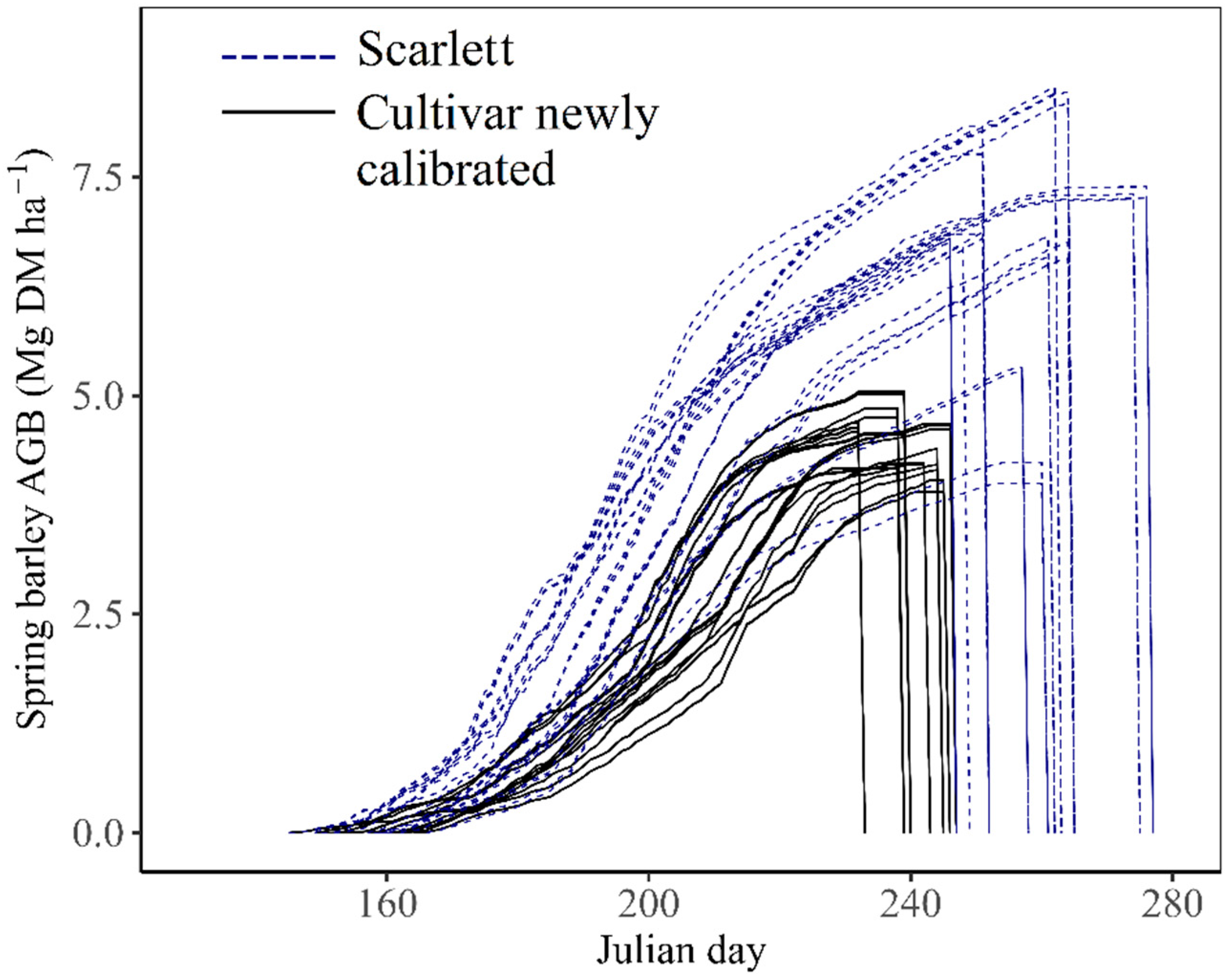
3.2. Calibration to Add New Cultivar Adapted to Northeastern Quebec Conditions in STICS

Default parameter values for the European reference cultivar (Scarlett) defined in STICS and newly calibrated parameter values for the Chapais spring barley cultivar adapted to the short growing season area are presented in Table 4. Based on the literature and our experimental data, the sum of GDD from emergence to the beginning of grain filling (stlevdrp) was reduced to 800 °C d and the duration of grain filling (stdrpmat) was reduced to 565 °C d (Table 4). Thus, the sum of GDD between emergence and physiological maturity (stlevdrp + stdrpmat) decreased from 1555 °C d for the Scarlett cultivar to 1365 °C d for the Chapais cultivar.
Predictions of LAI dynamics were not assessed because measured LAI data were not available. To improve the overestimated AGB predictions obtained with the default parameters, we set out to optimize the parameters controlling LAI dynamics (dlaimaxbrut, stlevamf, stamflax, durvief, and innsen) (Table 4). The maximum rate of leaf growth during LAI development (dlaimaxbrut) decreased. The sum of GDD between emergence and the end of the juvenile stage (stlevamf) and between the end of the juvenile stage and the maximum LAI (stamflax) both increased by 80 °C d relative to the default values after the optimization procedure. Therefore, the maximum LAI occurred at about 900 °C d after emergence. The parameters describing potential RUE (efcroijuv, efcroiveg, and efcroirepro), which is used for the calculation of shoot biomass, were also reduced (Table 4).
When the default parameters of the Scarlett cultivar were used, AGB was poorly predicted and largely overestimated with NME = −42% (Table S3). Differences in AGB accumulation and crop cycle duration between the Scarlett and the Chapais cultivars (Figure 2) reflect the overall effects of differences in the cultivars’ phenological parameters. For the same seeding date, the Chapais cultivar reached maturity on average 18 days earlier than the Scarlett cultivar under the conditions of northeastern Canada. On average for the seven years and the four management units, the predicted AGB was 4.4 ± 0.3 Mg DM ha−1 for the Chapais cultivar and 6.4 ± 1.0 Mg DM ha−1 for the Scarlett cultivars, respectively. This reduction in AGB for the northeastern Canada cultivar resulted from the decrease in the parameters relative to the maximum rate of daily increase in LAI and the potential RUE. In addition, the vitircarb and vitirazo values were adjusted (Table 4) to increase the annual GY and NCG values, respectively, which were underestimated with the Scarlett parameters (NME = 16% and 38%, respectively).

3.3. Comparison between Observed and Predicted Values

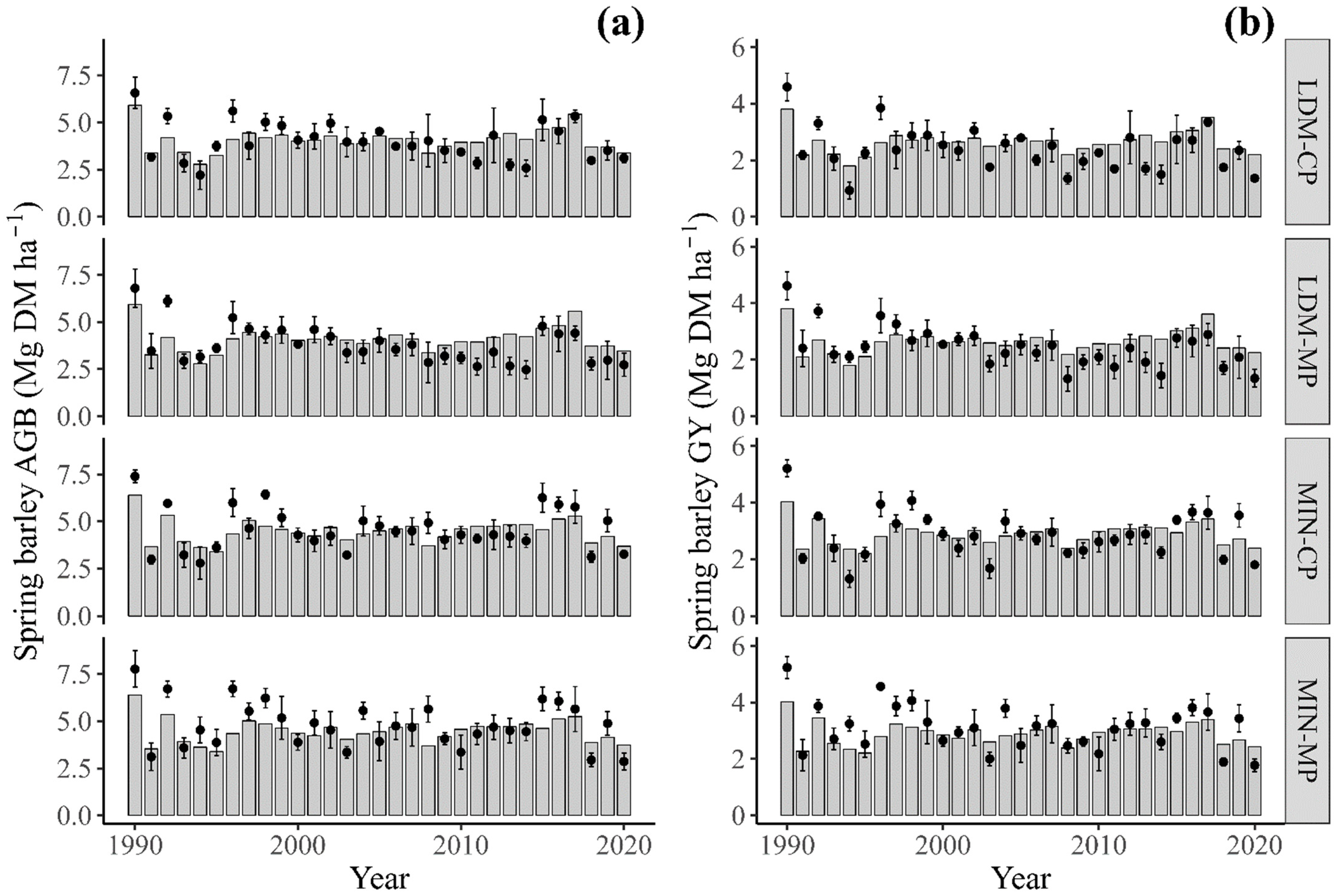
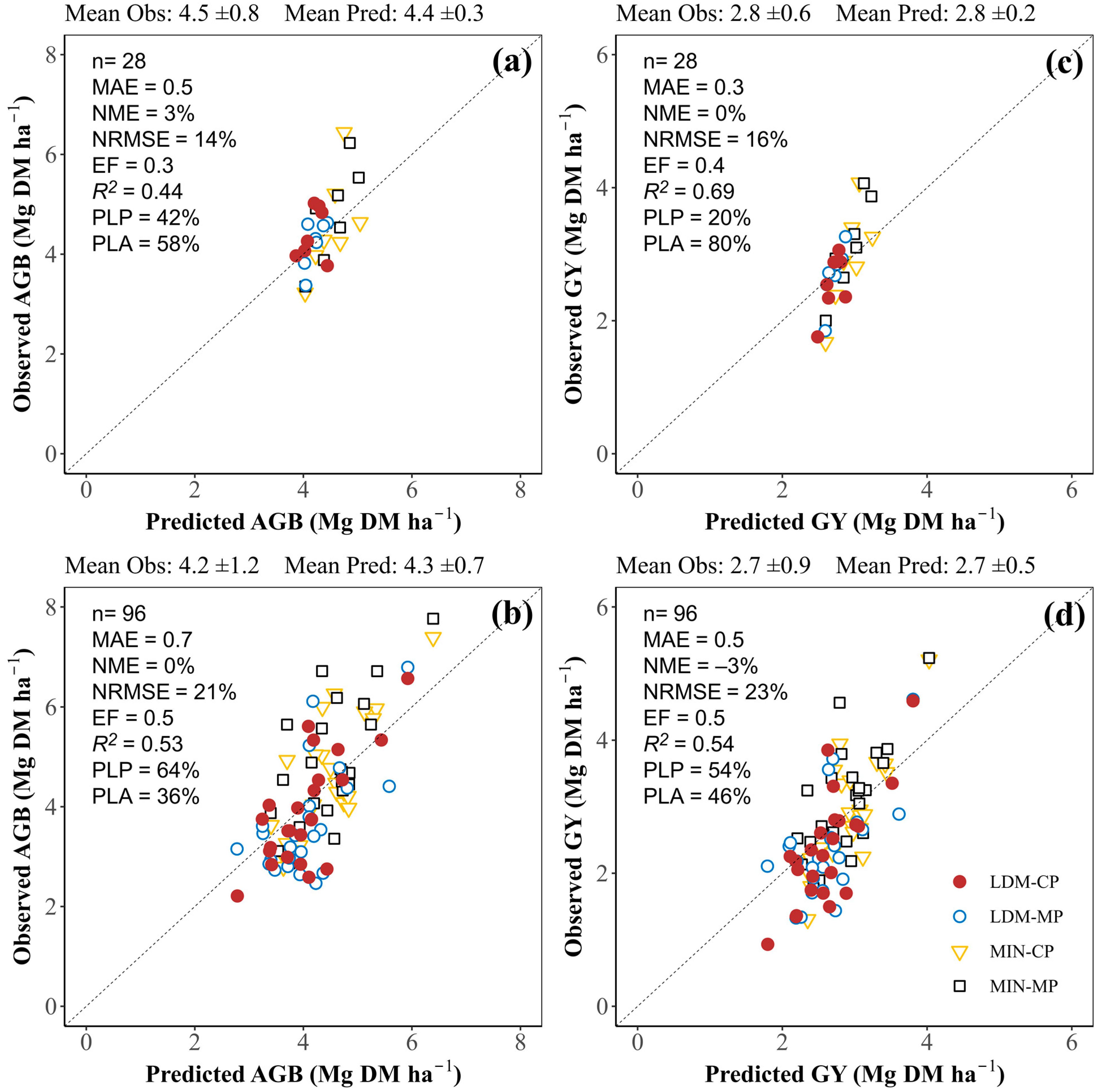
3.3.1. Aboveground Biomass and Grain Yield at Harvest

The observed AGB values for all treatments over 31 years of the cropping experiment ranged from 2.2 to 7.8 Mg DM ha−1yr−1 with a mean of 4.3 ± 1.2 Mg DM ha−1yr−1, whereas the predicted AGB values ranged from 2.8 to 6.4 Mg DM ha−1yr−1 with a mean of 4.3 ± 0.6 Mg DM ha−1yr−1 (Figure 3a). The mean of observed GY values was 2.7 ± 0.8 and the mean of predicted GY values was 2.8 ± 0.4 Mg DM ha−1 yr−1 (Figure 3b), with a narrower range for predicted values (1.8–4.0) than for the observed values (0.9–5.2).
After the calibration, STICS performed well in predicting AGB and GY with a low bias (NME = 3% and 0%, respectively), good NRMSE (14% and 16%, respectively), and moderate R2 (0.44 and 0.69, respectively) (Figure 4a,c). The STICS evaluation with the 24 remaining cropping years gave a similar performance for AGB and GY with a low bias (NME = 0% and −3%, respectively), a small NRMSE (21% and 23%, respectively), a moderate R2 and a satisfactory EF (Figure 4b,d).
The error decomposition indicated that, for the evaluation dataset, the model errors for AGB and GY are due to dispersion error rather than systematic error (PLP > PLA); however, the opposite was true for the calibration dataset (Figure 4).

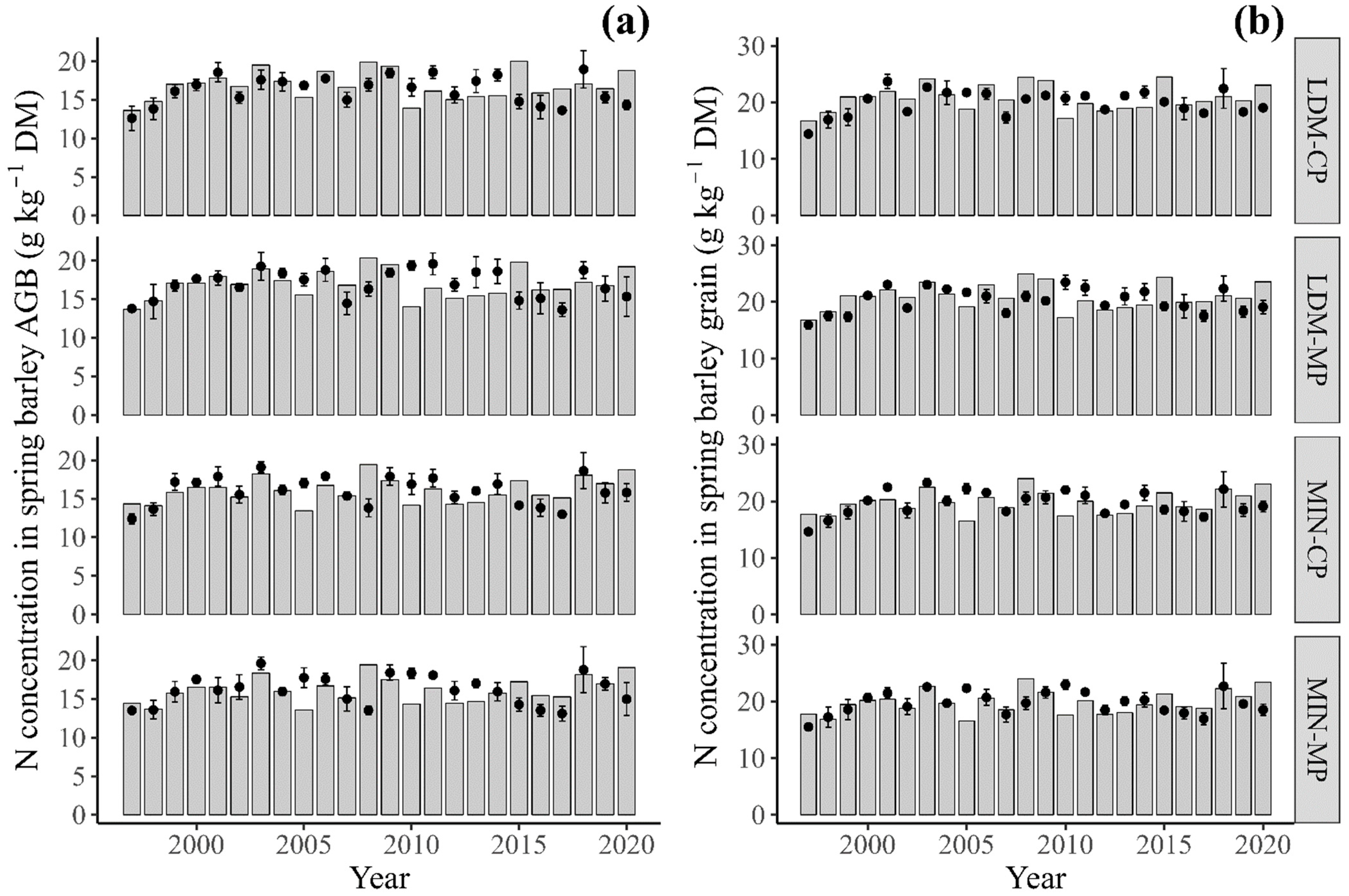
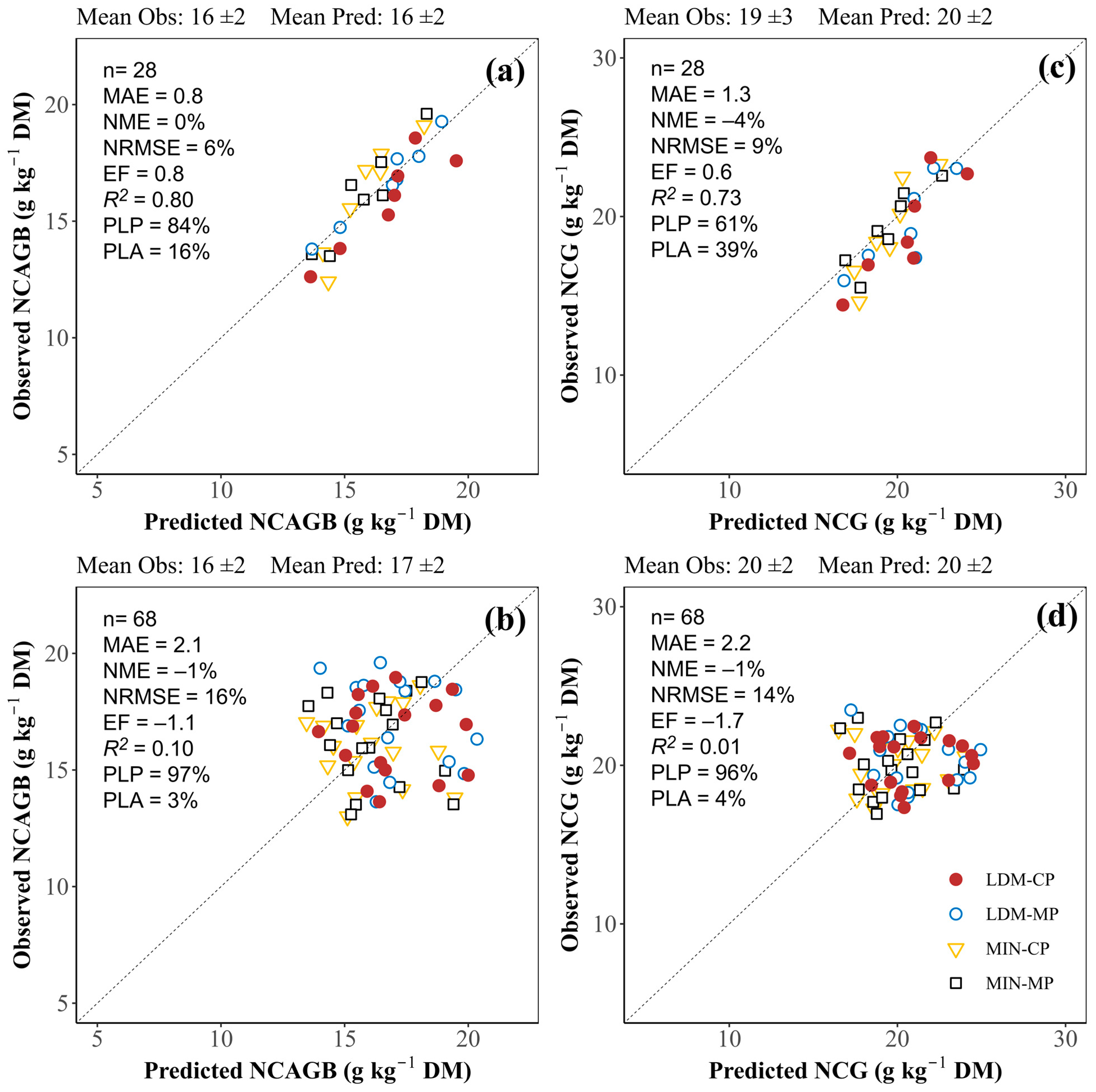
3.3.2. Nitrogen Concentration in Aboveground Biomass and in Grain at Harvest

Annual values of observed NCAGB at harvest over 24 years of measurement for the four treatments ranged from 12 to 20 g kg−1 DM with a mean of 16 ± 2 g kg−1 DM (Figure 5a). The mean (17 ± 2 g kg−1 DM) and the range (13–20 g kg−1 DM) of predicted NCAGB values were very close to the observed values. For NCG, the annual observed values ranged from 14 to 24 g kg−1 DM with a mean of 20 ± 2 g kg−1 DM. The range (17–25 g kg−1 DM) and the mean (20 ± 2 g kg−1 DM) of the annual predicted NCG values were also quite similar to the observed values (Figure 5b).
Calibration led to good prediction of NCAGB and NCG with a low relative bias, excellent NRMSE, and satisfactory EF; however, R2 was moderate for NCAGB and substantial for NCG, respectively (Figure 6a,c). For the evaluation dataset, the relative bias and the NRMSE were low (NME = −1% and NRMSE ≤ 16%) but the EF was negative and R2 was very weak for both variables (Figure 6b,d). The error decomposition showed that most of the error for NCAGB and NCG was due to dispersion (PLP > PLA), for both datasets (Figure 6).

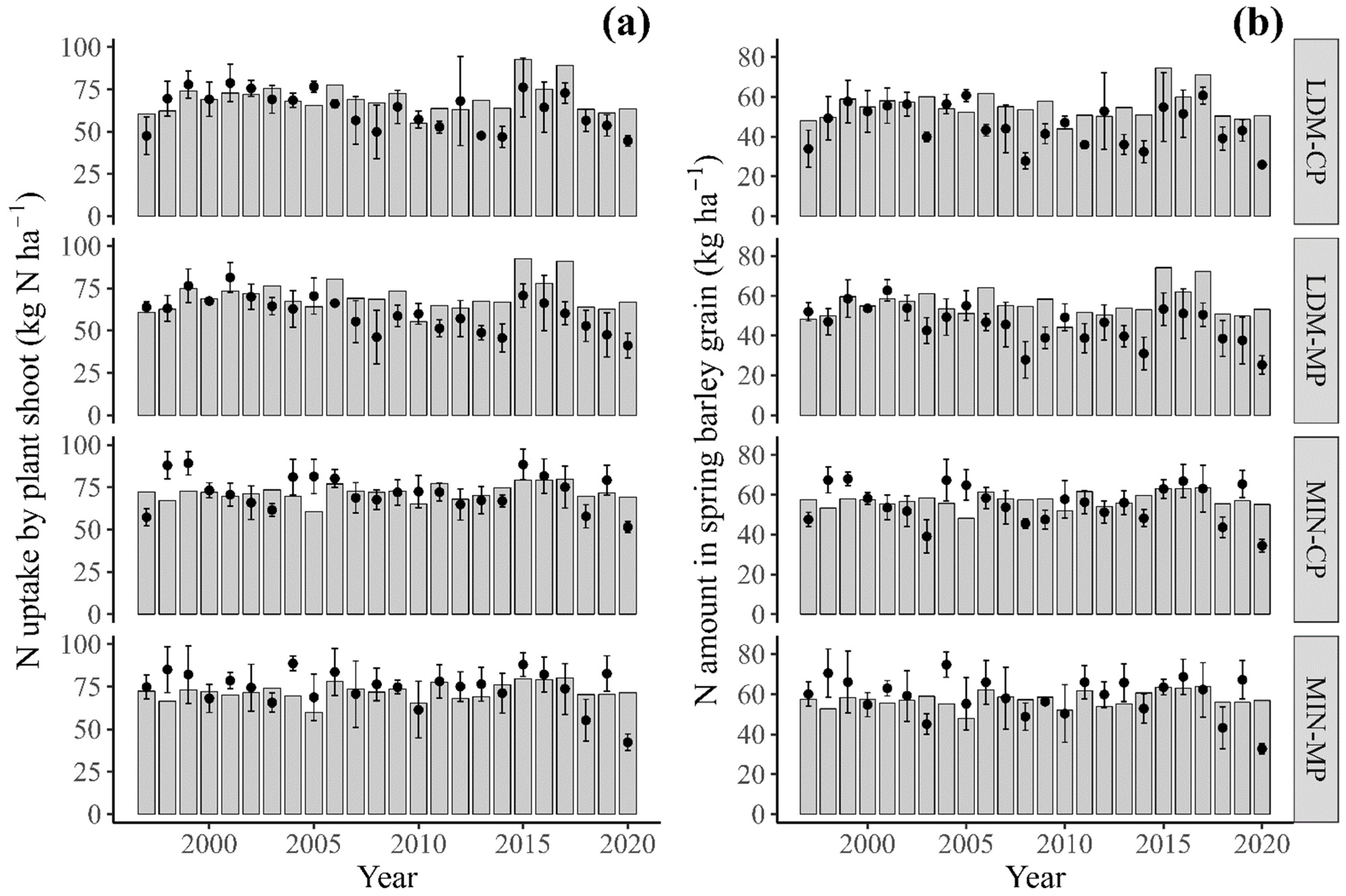
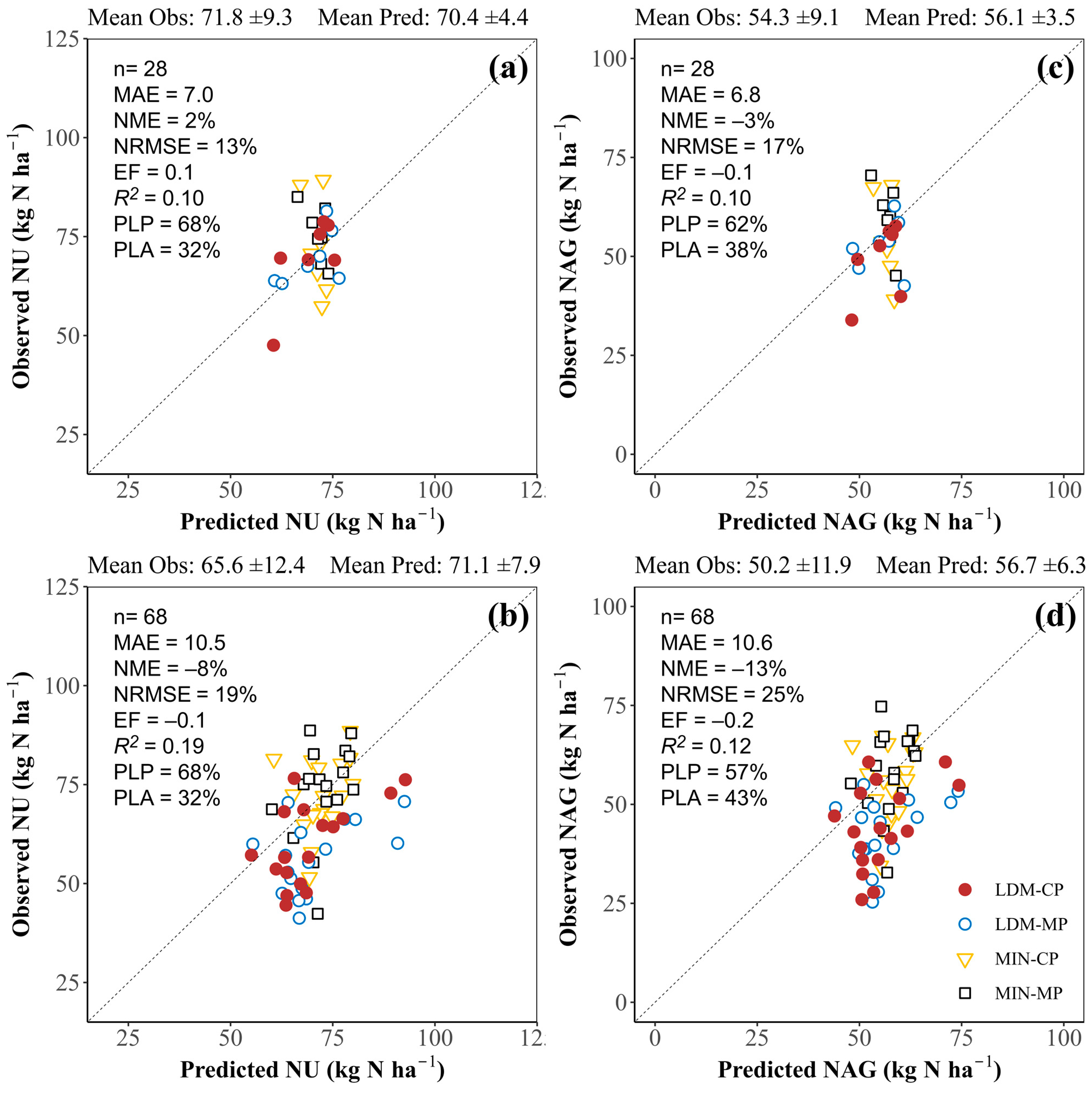
3.3.3. Plant N Uptake and Amount of N in Grain

The mean observed NU value for the 24 years of cropping and four treatments was 67.4 ± 11.9 kg N ha−1yr−1 with values ranging from 41.2 to 89.3 kg ha−1yr−1. In comparison, the predicted NU ranged from 55.1 to 92.8 kg ha−1yr−1 with a mean of 70.9 ± 7.0 kg ha−1yr−1 (Figure 7a). The mean observed NAG value was 51.4 ± 11.2 kg N ha−1yr−1 with values ranging from 25.3 to 74.7 kg N ha−1yr−1 (Figure 7b). For the predicted NAG, there was a narrower range of values (43.9–74.4 kg N ha−1yr−1) but the mean (56.5 ± 5.6 kg N ha−1yr−1) was similar compared to observed values.
According to the statistical criteria, NU predictions were satisfactory for the calibration and the evaluation dataset, with a small NRMSE (13% and 19%, respectively) and low bias (NME = 2% and −8%, respectively) but relatively low EF and R2 (Figure 8a,b). The NAG predictions were satisfactory for the calibration dataset, with a good NRMSE and a low bias, but a negative EF (−0.1) (Figure 8c). For the evaluation dataset, the NRMSE was fair (25%), and the EF and R2 were weak (Figure 8d). The relative contributions to the model error for NU and NAG indicate that most of the error was due to dispersion, for both datasets (PLP ≥ 57%) (Figure 8).

3.4. STICS Performance in Relation to Climatic Conditions

STICS identified a slight degree of anoxia stress in the majority of cropping years in this study. This may be due to the soil texture (silty clay), which has a low infiltration capacity, and the high-intensity rainfall events in the region. Five of the 24 years in the evaluation dataset were not subject to anoxic conditions (exofac = 0), but they were subject to water deficit stress. The other years had waterlogged conditions which varied in intensity and duration depending on the amount and distribution of rainfall over the growing season. Situations with 0 < exofac < 0.06 were observed for 9 of the 24 years and situations with 0.06 ≤ exofac < 0.14 for 10 of the 24 years. Conditions with 0 < exofac < 0.06 correspond approximately to years with evenly distributed rainfall throughout the growing season and close to the average level of rainfall over 31 years of experimentation (317 mm) (Table S1).
Predictions of the variables of interest were better for years with a low waterlogging index (0 < exofac < 0.06), giving small biases (|NME| < 7%), NRMSE values ranging from 10% to 22%, and high EF, except for NAG (Table 5). Under water deficit conditions, relatively higher NME values (|NME| ≥ 8%) were obtained for biomass accumulation variables and lower values for the amount of N in plant shoots and grain. The opposite was true for conditions with a significant waterlogging index. EF values were negative for all variables simulated under water deficit conditions. The NRMSE values were greater when the waterlogging index was high (exofac ≥ 0.06). The other climate variables such as temperature, GDD, and global radiation varied from year to year but appear not to have affected the performance of STICS in predicting AGB, GY, NCAGB, NCG, NU, and NAG.

4. Discussion

4.1. STICS Calibration for Spring Barley Cultivars Adapted to Climatic Conditions of Northeastern Quebec

The biomass and plant N uptake of a spring barley cultivar adapted to pedoclimatic conditions of the Saguenay–Lac-Saint-Jean region (northeastern Quebec) had never been simulated with STICS. Our results for spring barley confirm that the model can be successfully calibrated for a new cultivar and new pedoclimatic conditions such as those found in northeastern Quebec. This is consistent with the results previously reported for soybean and spring wheat cultivars [37] as well as for maize cultivars [39].
Although the calibration was based on a limited set of target variables, all of them measured at the end of the growing season, it significantly improved the simulation of biomass accumulation and N nutrition for spring barley cultivars grown in silty clay soil at Normandin. This is consistent with the findings of Guillaume et al. [56] that STICS can be calibrated without integrating additional observed data from sequential sampling during the growing season to improve the prediction of crop variables at harvest (e.g., AGB and GY). However, this is not always the case for other crop models where restricted calibration can create substantial uncertainty in crop growth predictions [25,28].
Although the calibration procedure should give priority to adjusting parameters by using direct measurements and data from the literature, this is not always possible, for many reasons [62]. In this study, crop height and yield component traits were adjusted according to data found in the literature, and other parameter values were derived from the sequential optimization performed using observed values. This underscores the importance of ensuring that the values of the parameters calibrated by optimization are plausible. The sum of GDD between emergence and physiological maturity obtained during calibration falls in the range of GDD values (1268 to 1702 °C d) reported for spring barley grown at three locations in the northern Great Plains of the Canadian province of Alberta (Botha, Lacombe, and Olds) from 1993 to 1996 [11] as well as in the range of values (1250 to 1850 °C d) reported for barley grown in agricultural area of the western Canadian province of Manitoba [70]. The reduction of stlevdrp and stdrpmat is consistent with the shorter growing season characterizing the study location in northeastern Quebec. In addition, the sum of GDD required to reach maximum LAI is in line with results from Alberta, where reported values ranged from 756 to 1109 °C d, depending on site location, year, and cultivar [11]. Furthermore, it is generally expected that post-anthesis RUE (efcroirepro) will be equal to or lower than pre-anthesis RUE (efcroiveg) since no new leaves are produced after heading and the photosynthetic activity of existing leaves decreases with age [71,72]. However, Raj Singh et al. [73] found that RUE for spring barley is not constant throughout the growing season. It has also been reported that post-anthesis RUE values can be high for six-row barley under short-growing season conditions: 1.6 to 3.0 g DM MJ−1 for pre-anthesis RUE vs. 2.1 to 3.8 g DM MJ−1 for post-anthesis RUE [74,75]. This higher post-anthesis RUE value can be attributed to the significant contribution of the cereal spike to photosynthetically active radiation interception (PAR) and to grain yield [76,77,78]. Furthermore, Zhang et al. [78] suggested that RUE for cereal spike (spike light interception) should be included in crop models in addition to the RUE derived from leaf light interception in order to capture the contribution of spike photosynthesis to grain yield and to improve simulation results, notably in the high yield range. For STICS, the interception of PAR by cereal spikes has not been explicitly documented.

4.2. STICS Performance

After the calibration using 28 predicted/observed data pairs (7 years × 4 treatments) of the dataset, the ability of STICS to predict AGB, GY, NCAGB, NCG, NU, and NAG (Figure 4, Figure 6 and Figure 8) was tested with the remaining 96 predicted/observed data pairs (24 years × 4 treatments) by regressing field-observed vs. STICS-predicted values using the standard major axis procedure proposed recently by Correndo et al. [61].
The NRMSE values for AGB (Figure 4a,b) were low compared to those reported in previous studies where STICS was used for European spring barley cultivars (NRMSE of about 25–35%) [23,36]. For GY (Figure 4c,d), the NRMSE values were in the same range as those obtained by Rötter et al. (2012) (NRMSE = 24%) in northern and central Europe and by Salo et al. [17] (NRMSE = 10–26%) in southern Finland. For NCG, the NRMSE values of 9% and 14% for calibration and evaluation, respectively, were low compared to the values obtained by Salo et al. [17] (NRMSE = 13–27%) and Yin et al. [25] (NRMSE > 30%) for spring barley. Our results for NU prediction were comparable to those reported for spring wheat grown at three locations in the Mixedwood Plains Ecozone of eastern Canada (Quebec and Ontario) (NRMSE = 14–20%) [79]. In general, plant N attribute variables are more difficult to model than plant biomass. The simulation of these variables is closely dependent at the same time on the simulation of biomass as well as the dynamic of mineral N in the soil, which is itself the result of multiple simultaneous biotransformation processes that interact with several other parameters.
With respect to error decomposition, it has been reported that complex models with a large number of parameters generally tend to have a low systematic error but a large dispersion error [80]. In their overall performance evaluation, Coucheney et al. [33] concluded that STICS errors are mostly related to dispersion error rather than systematic error, and this is also what we observed in our study.
The annual variability of biomass and N accumulation in plant parts was generally well captured, with predicted values being close to observed values, even several years after the start of the simulation. This indicates that STICS performed well in predicting spring barley production over 31 years in a continuous simulation mode without simulations being reset each year, which is consistent with the results of previous studies [25,32]. This was tested for the first time with STICS under northern climatic conditions with a heavy snow cover every winter. The model’s continuous simulation mode is especially useful for predicting the effects of climate change, which requires long-term simulations. In addition, the STICS evaluation showed that all the output variables were well predicted for the Alyssa cultivar, which has been used since 2015 in the long-term field experiment (Figure 3, Figure 5 and Figure 7). After a validation step using independent observations from other sites, the new set of calibrated parameters could be used for other cultivars in northeastern Quebec with characteristics similar to those of the Chapais and Alyssa cultivars. This aspect is important, especially since these cultivars are well adapted to the environmental conditions found in Canada, in both the eastern and western regions [46,81].
Overall, the STICS outputs reproduced the same trends as the observed data for the various treatments (Table S4). Concerning N sources, higher yields observed for the MIN than for the LDM treatment in this study contradict some observations that dairy manure can increase long-term soil fertility. Lafond et al. [45] found that LDM and MIN treatments can affect barley grain yields differently depending on the cropping system (rotation or monoculture). The mean predicted AGB and GY values were lower for the LDM treatment than for the MIN treatment. However, the model overestimated NU and NAG for the LDM treatment (Figure 7). Although the model predictions of AGB, GY, NCAGB, and NCG for the LDM treatment in 2011, 2013, and 2014 were poor, the predicted values were close to the observed values for all the other years (Figure 3 and Figure 5). For the tillage systems, the predicted values for the MP and CP treatments were comparable (Table S4). As is the case for most currently available models, the variables and processes simulated by STICS are still limited to the incorporation and redistribution of residues and nutrients in the soil down to the tillage depth. Yet, tillage affects soil functioning and, ultimately, crop yield through multiple processes such as microbial activity and biomass, weed seeds and soil texture redistribution, as well as soil hydraulic properties [82]. In addition, the differences in the observed values of some variables such as GY due to the tillage treatments were low (7%), even if statistically significant (Table 2). The two tillage treatments did not differ in the observed AGB values.

4.3. STICS Process-Based Model vs. Statistical Model

Given that the performance metrics from the cross-validation method are equal to the average of the performance metrics calculated for each of the 5 iterations (5 folds), we can state that the overall predictive performance of STICS obtained with the 2 datasets was comparable to that of the mixed model approach for all production attributes variables (Table 2, Figure 4, Figure 6 and Figure 8). The 2 models, which represent the two extremes of a spectrum of modeling approaches gave similar good performances although the process-based model STICS integrates both soil and plant processes as well as agri-environmental conditions. This is not surprising, since we only used the database from one experimental site. As well as the great flexibility in the type of input that can be used, the main advantage of the statistical model is that it relies solely on the data for its parameterization, by minimizing the difference between observed and predicted values of the training datasets. However, their results can not be extrapolated to new contexts. On the other hand, process-based approaches require a significant amount of input data to run, some processes are better understood than others, and calibration often requires a lot of time before achieving satisfactory performance predictions. Therefore, the sources of error in a process-based model can be multiple (model structure, model parameters, uncertainty in model inputs, uncertainty in evaluation/validation data) [83]. To be applied to broader conditions, although process-based models are theoretically universal in scope, as they are based on ecophysiological and biological laws, validation steps with independent data are needed to see how the model behaves outside the conditions under which it has been calibrated.

4.4. Suggestions to Improve Model Performance

The STICS evaluation indicated that predictions of plant variables were less accurate when the waterlogging index level was high (Table 5). For example, the large underestimation of AGB and GY that occurred in 1996 (Figure 3a,b) was partly due to the large amount of rainfall in July (200 mm), which induced transitory stress from waterlogging (exofac = 0.09 during the reproductive stage) that the model captured too intensely in the AGB growth and GY predictions. This suggests that some plant parameters related to root, LAI, or biomass growth are sensitive to excess water and, should be adjusted to improve the simulations under excessive water conditions. The assessment of the soil water content (at 0–20 cm depth) was carried out with the measured data collected on the adjacent plots belonging to the experimental set-up under spring barley and forage in 2011, a year characterized by above-average rainfall most of the growing season (402 mm), showed a very satisfactory soil water content prediction with an excellent NRMSE (9.8%), a satisfactory EF, and a moderate R2 (data not shown). In general, soil water content is one of the variables that is best predicted by the STICS model [33], and this is also true under eastern Canadian (Ontario and Quebec provinces) climatic conditions [19,84].
The predicted values of AGB and GY were much greater than the observed values for the LDM treatment in 2011, 2013, and 2014, but not for the MIN treatment (Figure 3). In contrast to the other years, STICS failed to reproduce the low observed values of AGB and GY in the LDM for these three cropping years. The observed AGB and GY values were the lowest, and the yield gap compared to the MIN treatment was particularly large. It has been reported that cereal GY in monoculture systems using organic fertilizers is lower than with a mineral fertilizer due to low N use efficiency [45,85]. Significant differences in observed AGB and GY values between the MIN and LDM treatments (Table 2, Figure S1) can also be explained by the proportion of mineral N, the mineralization rate of organic N in LDM, or poor synchronization of the availability of organic N in the soil for the critical phases of crop growth [86]. The amount of N applied as organic fertilizer in 2011, 2013 and 2014 was large compared with other years (103, 138, and 123 kg total N ha−1, respectively, with at least 30% in mineral form), and STICS output showed that predicted soil mineral N content down to the 100 cm depth was comparable between LDM and MIN in 2013 and 2014 (Figure S3). It is therefore likely that grain yields were affected and exacerbated by factors related to biotic pressures, which are not accounted for by STICS. The slight NCAGB and NCG underestimations can be explained in part by a dilution effect due to the strong overestimation of AGB and GY (Figure 3a,b), even though NU and NAG were overestimated for these years (Figure 7a,b). It would be interesting in the future to evaluate the model’s performance in simulating spring barley yield and N plant status in response to contrasting N application rates of a given fertilizer. In this study, the MIN (70 kg N ha−1 yr−1) and LDM (107 kg N ha−1 yr−1 corresponding to about 40 kg N ha−1 yr−1 of mineral N) treatments provided an amount of available N to the crop that differed slightly, taking into account immobilization of mineral N from mineral fertilizer (on average 15 kg N ha−1 yr−1) and net mineralization for the LDM treatment (on average 9 kg N ha−1 yr−1), as predicted by STICS.
To further refine consideration of the effect between MIN and LDM treatment, STICS could be further improved by taking better account of N supply. In this study, all the parameters of the model equations used to simulate soil N transformation processes are model default values adopted for temperate regions. In the absence of measured field data, the accuracy with which STICS simulates N transformation processes in the soil could not be assessed. These processes influence the dynamics of soil mineral N and its availability to plants [21,22]. Previous studies conducted on a sandy loam field near Quebec City (QC, Canada) cultivated with perennial timothy (Phleum pratense L.) showed that total soil mineral N was reasonably well simulated, although soil nitrate content was overestimated during a certain period of the crop cycle [84]. Assessing the ability of STICS to simulate N transformation processes under spring barley cropping systems in soils from northeastern Quebec province should be included in future studies. This lack of soil measurement data and the absence of observations from a different (independent) site constitute the main limitation of this study.
In 2005 and 2010, predicted NCAGB and NCG values were lower than the observed values for all treatments (Figure 5). Rainfall was significantly below the 31-year average for these two years, with only 176 and 179 mm of cumulative rainfall during the cropping period, respectively (Table S1). The crop was under water stress and STICS predicted low NU values (Figure 7a). Drought is known to affect the acquisition of nutrients by roots and their transport to shoots, resulting in reduced N uptake and plant N in barley [87,88]. STICS thus exaggerates the depressive effect of water stress on N nutrition. A study of spring wheat at three sites in the Mixedwood Plains Ecozone of eastern Canada showed that the model’s performance was sensitive to the amount of rainfall during the growing season [79]. It showed that the model’s performance was better when rainfall was close to normal in the early growing season.
Field data during the growing season (e.g., AGB and NCAGB) that could be used in the calibration procedure would help to further improve the prediction of AGB, GY, NCAGB, NGY, NU, and NAG. This would also make it possible to assess and adjust the prediction of NU during the crop vegetative stage and N remobilization/uptake during the grain filling period, as well as the effects of possible N stress. Kherif et al. [89] stated that the performance of soil–crop models refers not only to the overall accuracy of model predictions, but also to the ability of models to capture the temporal dynamics of plant and soil variables. The verification of LAI dynamics which plays a key role in predicting plant biomass accumulation and the validation of the critical N dilution curve parameters for spring barley may also be required to predict AGB and NU more precisely. Morissette et al. [40] concluded that using cultivar-specific N dilution curves instead of the default curve improves STICS performance and is essential for adequately predicting the N cycle of potato growing systems. To our knowledge, no critical N dilution curve for spring barley grown in agricultural soils from the six provinces of eastern Canada (New Brunswick, Newfoundland, Nova Scotia, Prince Edward Island, Quebec, and Ontario) has been established or at least validated to date. The default critical N dilution curve parameters used in this study are those proposed by Zhao [51] for winter barley from data obtained in China. For wheat, a specific critical N dilution curve was developed for spring wheat in Canada, which differed from the reference curve used for winter wheat in Europe [90]. For maize, the critical N dilution curve established in France was found to be valid in several agricultural sites within the province of Quebec [91], although Jégo et al. [92] have proposed a specific critical N dilution curve for Canada using the Bayesian approach for data analysis.

5. Conclusions

This study enabled us to calibrate STICS for spring barley cultivars grown on gleysolic soil under the climatic conditions (continental cold and humid climate) of Saguenay–Lac-Saint-Jean (northeastern Quebec). The STICS calibration procedure required the adjustment of cultivar parameters in particular, thus confirming the genericity of most plant parameters defined in STICS. Good agreement was obtained between annual observed and predicted values of AGB, GY, NCAGB, NCG, NU, and NAG during 31 years of spring barley monoculture, although there was a greater dispersion for the plant N attributes. STICS also reproduced the trends of observed values effectively with different tillage systems and N sources applied at the locally recommended N rates. Model errors were generally due to dispersion error rather than systematic error, indicating that the model was correctly parameterized. Although the simulation results for the spring barley grown at the studied experimental site were satisfactory, they could be improved with additional data, particularly data obtained during the growing season to capture the temporal dynamics of plant and soil variables. The validation of the STICS predictions for the temporal dynamics of spring barley growth and N uptake in response to various crop management approaches and contrasting soil types is also needed using observations from independent datasets obtained from different sites. Our results will serve as the basis for future studies aimed at understanding and quantifying long-term changes in C and N fluxes in cropping systems with spring barley in the same site and experimental set-up.

Supplementary Materials

The following supporting information can be downloaded at: https://www.mdpi.com/article/10.3390/agronomy13102540/s1. Table S1. Weather data during the cropping period of spring barley recorded at the Normandin and the Saint-Prime weather station of Environment Canada. Table S2. Key cropping practices and measurements at harvest of the 2 spring barley cultivars. Table S3. Performance of STICS with default parameters and newly calibrated parameters to predict spring barley aboveground biomass, grain yield, N concentration in aboveground biomass and grain, plant shoot N uptake, and N amount in grain. Table S4. Mean of field-observed and STICS-predicted values for aboveground biomass, grain yield, N concentration in aboveground biomass and grain, N uptake by plant, and N amount in grain as affected by N source type and tillage system. Figure S1. Aboveground biomass, grain yield, N concentration in aboveground biomass, N uptake by plant, and N amount in grain as affected by N source type or tillage system. Figure S2. Scatterplots showing the trend in field-observed spring barley aboveground biomass and grain yield as a function of N source type. Figure S3. STICS-predicted soil mineral N content down to 100 cm depth over 31 years according to management system.

Author Contributions

N.R.: conceptualization, methodology, data curation, formal analysis, writing—original draft. G.J., A.M. and A.K.: supervision, validation, writing—review and editing. C.M.: funding acquisition, supervision, validation, writing—review and editing. N.Z.: funding acquisition, resources, supervision, validation, writing—review and editing. J.L.: validation, writing—review and editing. All authors have read and agreed to the published version of the manuscript.

Funding

This research is funded by Agriculture and Agri-Food Canada’s A-base program and is supported by the French government’s “Eiffel Excellence Scholarship” (grant No. P769751A).

Data Availability Statement

Data generated or analyzed during this study are available from the corresponding author upon reasonable request.

Acknowledgments

We are deeply grateful to the dedicated staff of Agriculture and Agri-Food Canada at Normandin Experimental Farm for their fieldwork during the study. We also thank Gilles Bélanger for his excellent comments on an early draft of the manuscript.

Conflicts of Interest

The authors declare no conflict of interest.

References

  1. Ministère de l’Agriculture, des Pêcheries et de l’Alimentation du Québec. Sectoral Diagnostic Portrait of the Grain Industry in Quebec; Bibliothèque et Archives Nationales du Québec: Montréal, QC, Canada, 2020; 51p. (In French) [Google Scholar]
  2. Bulman, P.; Mather, D.E.; Smith, D.L. Genetic Improvement of Spring Barley Cultivars Grown in Eastern Canada from 1910 to 1988. Euphytica 1993, 71, 35–48. [Google Scholar] [CrossRef]
  3. Holland, J.; Brown, J.L.; MacKenzie, K.; Neilson, R.; Piras, S.; McKenzie, B.M. Over Winter Cover Crops Provide Yield Benefits for Spring Barley and Maintain Soil Health in Northern Europe. Eur. J. Agron. 2021, 130, 126363. [Google Scholar] [CrossRef]
  4. Statistics Canada. Estimated Area, Yield, Production, Average Farm Price and Total Farm Value of Major Field Crops, in Metric and Imperial Units. 2008. Available online: https://www.pgq.ca/articles/services-dinformation-sur-les-marches/portrait-quebec/production-quebec/ (accessed on 13 January 2023).
  5. Friedt, W.; Horsley, R.D.; Harvey, B.L.; Poulsen, D.M.; Lance, R.C.; Ceccarelli, S.; Grando, S.; Capettini, F. Barley Breeding History, Progress, Objectives, and Technology. In Barley: Production, Improvement, and USES; Blackwell Publishing: Hoboken, NJ, USA, 2011; pp. 160–220. [Google Scholar]
  6. Bélanger, G.; Bootsma, A. Impacts of climate change on agriculture in Quebec [Paper presentation]. In Proceedings of the Présentation au 65e congrès de l’Ordre des Agronomes du Québec, Quebec, Sainte-Foy, 7–8 June 2002. 20p. (In French). [Google Scholar]
  7. Agriculture and Agri-Food Canada. Effective Growing Degree Days—Quebec. 2010. Available online: https://publications.gc.ca/collections/collection_2018/aac-aafc/A59-55-2010-eng.pdf (accessed on 23 February 2023).
  8. Moore, T. Soils of Quebec. In Digging into Canadian Soils. An Introduction to Soil Science; Canadian Society of Soil Science: Pinawa, MB, Canada, 2021; pp. 401–409. [Google Scholar]
  9. Setter, T.L.; Burgess, P.; Waters, I.; Kuo, J. Genetic Diversity of Barley and Wheat for Waterlogging Tolerance in Western Australia. In Proceedings of the 9th Australian Barley Technical Symposium, Melbourne, VIC, Australia, 12–16 September 1999; Australian Barley Technical Symposium Inc.: Melbourne, VIC, Australia, 1999; pp. 1–7. [Google Scholar]
  10. Cao, W.; Moss, D.N. Temperature and Daylength Interaction on Phyllochron in Wheat and Barley. Crop Sci. 1989, 29, 1046–1048. [Google Scholar] [CrossRef]
  11. Juskiw, P.; Jame, Y.-W.; Kryzanowski, L. Phenological Development of Spring Barley in a Short-Season Growing Area. Agron, J. 2001, 93, 370–379. [Google Scholar] [CrossRef]
  12. Ma, B.L.; Smith, D.L. Apical Development of Spring Barley under Field Conditions in Northeastern North America. Crop Sci. 1992, 32, 144–149. [Google Scholar] [CrossRef]
  13. Russell, G. Barley Knowledge Base; Joint Research Centre: Brussels, Belgium, 1990; p. 135. [Google Scholar]
  14. Oteng-Darko, P.; Yeboah, S.; Addy, S.N.T.; Amponsah, S.; Danquah, E.O. Crop Modeling: A Tool for Agricultural Research—A Review. J. Agric. Res. Develop. 2013, 2, 1–6. [Google Scholar]
  15. Quintero, D.; Díaz, E. A Comparison of Two Open-Source Crop Simulation Models for a Potato Crop. Agron. Colomb. 2020, 38, 382–387. [Google Scholar] [CrossRef]
  16. Basso, B.; Cammarano, D.; Troccoli, A.; Chen, D.; Ritchie, J.T. Long-Term Wheat Response to Nitrogen in a Rainfed Mediterranean Environment: Field Data and Simulation Analysis. Eur. J. Agron. 2010, 33, 132–138. [Google Scholar] [CrossRef]
  17. Salo, T.J.; Palosuo, T.; Kersebaum, K.C.; Nendel, C.; Angulo, C.; Ewert, F.; Bindi, M.; Calanca, P.; Klein, T.; Moriondo, M. Comparing the Performance of 11 Crop Simulation Models in Predicting Yield Response to Nitrogen Fertilization. J. Agric. Sci. 2016, 154, 1218–1240. [Google Scholar] [CrossRef]
  18. Cheng, M.; Wang, H.; Fan, J.; Xiang, Y.; Liu, X.; Liao, Z.; Abdelghany, A.E.; Zhang, F.; Li, Z. Evaluation of AquaCrop Model for Greenhouse Cherry Tomato with Plastic Film Mulch under Various Water and Nitrogen Supplies. Agric. Water Manag. 2022, 274, 107949. [Google Scholar] [CrossRef]
  19. Saadi, S.; Pattey, E.; Jégo, G.; Champagne, C. Prediction of Rainfed Corn Evapotranspiration and Soil Moisture Using the STICS Crop Model in Eastern Canada. Field Crops Res. 2022, 287, 108664. [Google Scholar] [CrossRef]
  20. Lammoglia, S.-K.; Moeys, J.; Barriuso, E.; Larsbo, M.; Marín-Benito, J.-M.; Justes, E.; Alletto, L.; Ubertosi, M.; Nicolardot, B.; Munier-Jolain, N. Sequential Use of the STICS Crop Model and of the MACRO Pesticide Fate Model to Simulate Pesticides Leaching in Cropping Systems. Environ. Sci. Pollut. Res. 2017, 24, 6895–6909. [Google Scholar] [CrossRef] [PubMed]
  21. Yin, X.; Beaudoin, N.; Ferchaud, F.; Mary, B.; Strullu, L.; Chlébowski, F.; Clivot, H.; Herre, C.; Duval, J.; Louarn, G. Long-Term Modelling of Soil N Mineralization and N Fate Using STICS in a 34-Year Crop Rotation Experiment. Geoderma 2020, 357, 113956. [Google Scholar] [CrossRef]
  22. Yin, X.; Kersebaum, K.-C.; Beaudoin, N.; Constantin, J.; Chen, F.; Louarn, G.; Manevski, K.; Hoffmann, M.; Kollas, C.; Armas-Herrera, C.M.; et al. Uncertainties in Simulating N Uptake, Net N Mineralization, Soil Mineral N and N Leaching in European Crop Rotations Using Process-Based Models. Field Crops Res. 2020, 255, 107863. [Google Scholar] [CrossRef]
  23. Constantin, J.; Beaudoin, N.; Launay, M.; Duval, J.; Mary, B. Long-Term Nitrogen Dynamics in Various Catch Crop Scenarios: Test and Simulations with STICS Model in a Temperate Climate. Agric. Ecosyst. Environ. 2012, 147, 36–46. [Google Scholar] [CrossRef]
  24. Gardi, M.W.; Memic, E.; Zewdu, E.; Graeff-Hönninger, S. Simulating the Effect of Climate Change on Barley Yield in Ethiopia with the DSSAT-CERES-Barley Model. Agron. J. 2022, 114, 1128–1145. [Google Scholar] [CrossRef]
  25. Yin, X.; Kersebaum, K.C.; Kollas, C.; Manevski, K.; Baby, S.; Beaudoin, N.; Öztürk, I.; Gaiser, T.; Wu, L.; Hoffmann, M. Performance of Process-Based Models for Simulation of Grain N in Crop Rotations across Europe. Agric. Syst. 2017, 154, 63–77. [Google Scholar] [CrossRef]
  26. Pasquel, D.; Roux, S.; Richetti, J.; Cammarano, D.; Tisseyre, B.; Taylor, J.A. A Review of Methods to Evaluate Crop Model Performance at Multiple and Changing Spatial Scales. Precis. Agric. 2022, 23, 1489–1513. [Google Scholar] [CrossRef]
  27. Di Paola, A.; Valentini, R.; Santini, M. An Overview of Available Crop Growth and Yield Models for Studies and Assessments in Agriculture. J. Sci. Food Agric. 2016, 96, 709–714. [Google Scholar] [CrossRef]
  28. Rötter, R.P.; Palosuo, T.; Kersebaum, K.C.; Angulo, C.; Bindi, M.; Ewert, F.; Ferrise, R.; Hlavinka, P.; Moriondo, M.; Nendel, C. Simulation of Spring Barley Yield in Different Climatic Zones of Northern and Central Europe: A Comparison of Nine Crop Models. Field Crops Res. 2012, 133, 23–36. [Google Scholar] [CrossRef]
  29. Jame, Y.W.; Cutforth, H.W.; Selles, F.; Campbell, C.A.; Jedel, P.; Kryzanowski, L. Determine the Best Crop Management Option on Canadian Prairies with a Computerized Decision Support System. In Soils and Crops Workshop; University of Saskatchewan: Saskatoon, SK, Canada, 1997; pp. 356–363. [Google Scholar]
  30. Brisson, N.; Mary, B.; Ripoche, D.; Hélène Jeuffroy, M.; Ruget, F.; Nicoullaud, B.; Gate, P.; Devienne-Barret, F.; Antonioletti, R.; Durr, C.; et al. STICS: A Generic Model for the Simulation of Crops and Their Water and Nitrogen Balances. I. Theory and Parameterization Applied to Wheat and Corn. Agronomie 1998, 18, 311–346. [Google Scholar] [CrossRef]
  31. Brisson, N.; Gary, C.; Justes, E.; Roche, R.; Mary, B.; Ripoche, D.; Zimmer, D.; Sierra, J.; Bertuzzi, P.; Burger, P. An Overview of the Crop Model STICS. Eur. J. Agron. 2003, 18, 309–332. [Google Scholar] [CrossRef]
  32. Beaudoin, N.; Launay, M.; Sauboua, E.; Ponsardin, G.; Mary, B. Evaluation of the Soil Crop Model STICS over 8 Years against the “on Farm” Database of Bruyères Catchment. Eur. J. Agron. 2008, 29, 46–57. [Google Scholar] [CrossRef]
  33. Coucheney, E.; Buis, S.; Launay, M.; Constantin, J.; Mary, B.; de Cortázar-Atauri, I.G.; Ripoche, D.; Beaudoin, N.; Ruget, F.; Andrianarisoa, K.S. Accuracy, Robustness and Behavior of the STICS Soil–Crop Model for Plant, Water and Nitrogen Outputs: Evaluation over a Wide Range of Agro-Environmental Conditions in France. Environ. Model. Softw. 2015, 64, 177–190. [Google Scholar] [CrossRef]
  34. Lebonvallet, S. Quinoa Establishment and Its Culture Simulation on the Bolivian Altiplano. Ph.D. Thesis, Institut des Sciences et Industries du Vivant et de l’Environnement (Agro Paris Tech), Avignon, France, 2008. Available online: https://theses.hal.science/pastel-00003841/ (accessed on 26 January 2023). (In French, with English Abstract).
  35. Sierra, J.; Brisson, N.; Ripoche, D.; Noël, C. Application of the STICS Crop Model to Predict Nitrogen Availability and Nitrate Transport in a Tropical Acid Soil Cropped with Maize. Plant Soil 2003, 256, 333–345. [Google Scholar] [CrossRef]
  36. Corre-Hellou, G.; Faure, M.; Launay, M.; Brisson, N.; Crozat, Y. Adaptation of the STICS Intercrop Model to Simulate Crop Growth and N Accumulation in Pea–Barley Intercrops. Field Crops Res. 2009, 113, 72–81. [Google Scholar] [CrossRef]
  37. Jégo, G.; Pattey, E.; Bourgeois, G.; Morrison, M.J.; Drury, C.F.; Tremblay, N.; Tremblay, G. Calibration and Performance Evaluation of Soybean and Spring Wheat Cultivars Using the STICS Crop Model in Eastern Canada. Field Crops Res. 2010, 117, 183–196. [Google Scholar] [CrossRef]
  38. Jégo, G.; Chantigny, M.; Pattey, E.; Bélanger, G.; Rochette, P.; Vanasse, A.; Goyer, C. Improved Snow-Cover Model for Multi-Annual Simulations with the STICS Crop Model under Cold, Humid Continental Climates. Agric. For. Meteorol. 2014, 195–196, 38–51. [Google Scholar] [CrossRef]
  39. Jégo, G.; Pattey, E.; Bourgeois, G.; Drury, C.F.; Tremblay, N. Evaluation of the STICS Crop Growth Model with Maize Cultivar Parameters Calibrated for Eastern Canada. Agron. Sust. Dev. 2011, 31, 557–570. [Google Scholar] [CrossRef]
  40. Morissette, R.; Jégo, G.; Bélanger, G.; Cambouris, A.N.; Nyiraneza, J.; Zebarth, B.J. Simulating Potato Growth and Nitrogen Uptake in Eastern Canada with the STICS Model. Agron. J. 2016, 108, 1853–1868. [Google Scholar] [CrossRef]
  41. Jégo, G.; Bélanger, G.; Tremblay, G.F.; Jing, Q.; Baron, V.S. Calibration and Performance Evaluation of the STICS Crop Model for Simulating Timothy Growth and Nutritive Value. Field Crops Res. 2013, 151, 65–77. [Google Scholar] [CrossRef]
  42. Ministère de l’agriculture, des pêcheries et de l’alimentation du Québec. Saguenay-Lac-Saint-Jean Agri-Food Portrait 2010; M. de l’agriculture, des pêcheries et de l’alimentation, Ed.; Direction Régionale du Saguenay-Lac-Saint-Jean: Saguenay, QC, Canada, 2014. (In French) [Google Scholar]
  43. Lapointe, R. Profil 2005 de La Production Agricole de La Région Du Saguenay-Lac-Saint-Jean; M. de l’agriculture, des pêcheries et de l’alimentation, Ed.; Direction Régionale du Saguenay-Lac-Saint-Jean: Saguenay, QC, Canada, 2006. [Google Scholar]
  44. Agriculture and Agri-Food Canada. The Normandin Research Farm in Quebec Looks to the Future. Government of Canada. Available online: https://agriculture.canada.ca/en/agri-info/normandin-research-farm-quebec-looks-future (accessed on 23 September 2023).
  45. Lafond, J.; Angers, D.A.; Pageau, D.; Lajeunesse, J. Sustainable Cereal and Forage Production in Dairy-Based Cropping Systems. Can. J. Plant Sci. 2016, 97, 473–485. [Google Scholar] [CrossRef]
  46. Kong, D.; Choo, T.M.; Narasimhalu, P.; Jui, P.; Ferguson, T.; Therrien, M.C.; Ho, K.M.; May, K.W. Genetic Variation and Adaptation of 76 Canadian Barley Cultivars. Can. J. Plant Sci. 1994, 74, 737–744. [Google Scholar] [CrossRef]
  47. Isaac, R.A.; Johnson, W.C. Determination of Total Nitrogen in Plant Tissue, Using a Block Digestor. J. Assoc. Off. Anal. Chem. 1976, 59, 98–100. [Google Scholar] [CrossRef]
  48. Beaudoin, N.; Lecharpentier, P.; Ripoche, D.; Strullu, L.; Mary, B.; Leonard, J.; Launay, M.; Justes, E. STICS Soil-Crop Model. Conceptual Framework, Equations and Uses; Éditions Quæ: Versailles, France, 2022. [Google Scholar]
  49. Brisson, N. Conceptual Basis, Formalisations and Parameterization of the STICS Crop Model; Éditions Quæ: Versailles, France, 2008. [Google Scholar]
  50. Lemaire, G.; Jeuffroy, M.-H.; Gastal, F. Diagnosis Tool for Plant and Crop N Status in Vegetative Stage: Theory and Practices for Crop N Management. Eur. J. Agron. 2008, 28, 614–624. [Google Scholar] [CrossRef]
  51. Zhao, B. Determining of a Critical Dilution Curve for Plant Nitrogen Concentration in Winter Barley. Field Crops Res. 2014, 160, 64–72. [Google Scholar] [CrossRef]
  52. Nicolardot, B.; Recous, S.; Mary, B. Simulation of C and N Mineralisation during Crop Residue Decomposition: A Simple Dynamic Model Based on the C:N Ratio of the Residues. Plant Soil 2001, 228, 83–103. [Google Scholar] [CrossRef]
  53. Saxton, K.E.; Rawls, W.J. Soil Water Characteristic Estimates by Texture and Organic Matter for Hydrologic Solutions. Soil Sci. Soc. Am. J. 2006, 70, 1569–1578. [Google Scholar] [CrossRef]
  54. Malhi, S.S.; Johnston, A.M.; Loeppky, H.; Vera, C.L.; Beckie, H.J.; Bandara, P.M.S. Immediate Effects of Time and Method of Alfalfa Termination on Soil Mineral Nitrogen, Moisture, Weed Control, and Seed Yield, Quality, and Nitrogen Uptake. J. Plant Nutr. 2007, 30, 1059–1081. [Google Scholar] [CrossRef]
  55. Martel, Y.A.; Lasalle, P. Radiocarbon Dating of Organic Matter from a Cultivated Topsoil in Eastern Canada. Can. J. Soil. Sci. 1977, 57, 375–377. [Google Scholar] [CrossRef]
  56. Guillaume, S.; Bergez, J.-E.; Wallach, D.; Justes, E. Methodological Comparison of Calibration Procedures for Durum Wheat Parameters in the STICS Model. Eur. J. Agron. 2011, 35, 115–126. [Google Scholar] [CrossRef]
  57. Hickey, L.T.; Germán, S.E.; Pereyra, S.A.; Diaz, J.E.; Ziems, L.A.; Fowler, R.A.; Platz, G.J.; Franckowiak, J.D.; Dieters, M.J. Speed Breeding for Multiple Disease Resistance in Barley. Euphytica 2017, 213, 64. [Google Scholar] [CrossRef]
  58. Buis, S.; Wallach, D.; Guillaume, S.; Varella, H.; Lecharpentier, P.; Launay, M.; Guerif, M.; Bergez, J.-E.; Justes, E. The STICS Crop Model and Associated Software for Analysis, Parameterization, and Evaluation. Methods Introd. Syst. Models Agric. Res. 2011, 2, 395–426. [Google Scholar] [CrossRef]
  59. Pinheiro, J.; Bates, D.; DebRoy, S.; Sarkar, D.; R Core Team. nlme: Linear and Nonlinear Mixed Effects Models. Available online: https://cran.r-project.org/package=nlme (accessed on 22 September 2023).
  60. Alfons, A.; cvTools: Cross-Validation Tools for Regression Models. Vignette, R Foundation for Statistical Computing. Available online: https://cran.r-project.org/web/packages/cvTools/cvTools.pdf (accessed on 22 September 2023).
  61. Correndo, A.A.; Hefley, T.J.; Holzworth, D.P.; Ciampitti, I.A. Revisiting Linear Regression to Test Agreement in Continuous Predicted-Observed Datasets. Agric. Syst. 2021, 192, 103194. [Google Scholar] [CrossRef]
  62. Falconnier, G.N.; Journet, E.-P.; Bedoussac, L.; Vermue, A.; Chlébowski, F.; Beaudoin, N.; Justes, E. Calibration and Evaluation of the STICS Soil-Crop Model for Faba Bean to Explain Variability in Yield and N2 Fixation. Eur. J. Agron. 2019, 104, 63–77. [Google Scholar] [CrossRef]
  63. Jamieson, P.D.; Porter, J.R.; Wilson, D.R. A Test of the Computer Simulation Model ARCWHEAT1 on Wheat Crops Grown in New Zealand. Field Crops Res. 1991, 27, 337–350. [Google Scholar] [CrossRef]
  64. Piñeiro, G.; Perelman, S.; Guerschman, J.P.; Paruelo, J.M. How to Evaluate Models: Observed vs. Predicted or Predicted vs. Observed? Ecol. Model. 2008, 216, 316–322. [Google Scholar] [CrossRef]
  65. Correndo, A.A.; Hefley, T.; Holzworth, D.P.; Ciampitti, I.A. R-Code Tutorial: Revisiting Linear Regression to Test Agreement in Continuous Predicted-Observed Datasets. Harvard Dataverse 2021. [Google Scholar] [CrossRef]
  66. Ho, K.M.; Choo, T.M.; Martin, R.A. AC Maple Barley. Can. J. Plant Sci. 2002, 82, 93–94. [Google Scholar] [CrossRef]
  67. Ho, K.M.; Seaman, W.L.; Choo, T.M.; Martin, R.A.; Rowsell, J.; Guillemette, L.; Dion, Y.; Rioux, S. AC Legend Barley. Can. J. Plant Sci. 2000, 80, 113–115. [Google Scholar] [CrossRef]
  68. Ho, K.M.; Seaman, W.L.; Choo, T.M.; Martin, R.A. AC Hamilton Barley. Can. J. Plant Sci. 1995, 75, 697–698. [Google Scholar] [CrossRef]
  69. Spaner, D.; Todd, A.G.; McKenzie, D.B. The Effect of Seeding Rate and Nitrogen Fertilization on Barley Yield and Yield Components in a Cool Maritime Climate. J. Agron. Crop Sci. 2001, 187, 105–110. [Google Scholar] [CrossRef]
  70. Mapfumo, E.; Chanasyk, D.S.; Puurveen, D.; Elton, S.; Acharya, S. Historic Climate Change Trends and Impacts on Crop Yields in Key Agricultural Areas of the Prairie Provinces in Canada: A Literature Review. Can. J. Plant Sci. 2023, 103, 243–258. [Google Scholar] [CrossRef]
  71. Calderini, D.F.; Dreccer, M.F.; Slafer, G.A. Consequences of Breeding on Biomass, Radiation Interception and Radiation-Use Efficiency in Wheat. Field Crops Res. 1997, 52, 271–281. [Google Scholar] [CrossRef]
  72. Gallagher, J.N.; Biscoe, P.V. Radiation Absorption, Growth and Yield of Cereals. J. Agric. Sci. 1978, 91, 47–60. [Google Scholar] [CrossRef]
  73. Raj Singh, D.S.; Biswas, B.; Mani, J.K. Radiation Interception and Radiation Use Efficiency in Barley. J. Agrometeorol. 2012, 14, 358–362. [Google Scholar]
  74. Bingham, I.J.; Blake, J.; Foulkes, M.J.; Spink, J. Is Barley Yield in the UK Sink Limited?: I. Post-Anthesis Radiation Interception, Radiation-Use Efficiency and Source–Sink Balance. Field Crops Res. 2007, 101, 198–211. [Google Scholar] [CrossRef]
  75. Muurinen, S.; Peltonen-Sainio, P. Radiation-Use Efficiency of Modern and Old Spring Cereal Cultivars and Its Response to Nitrogen in Northern Growing Conditions. Field Crops Res. 2006, 96, 363–373. [Google Scholar] [CrossRef]
  76. Ahmadi, A.; Joudi, M.; Janmohammadi, M. Late Defoliation and Wheat Yield: Little Evidence of Post-Anthesis Source Limitation. Field Crops Res. 2009, 113, 90–93. [Google Scholar] [CrossRef]
  77. Maydup, M.L.; Antonietta, M.; Guiamet, J.J.; Tambussi, E.A. The Contribution of Green Parts of the Ear to Grain Filling in Old and Modern Cultivars of Bread Wheat (Triticum Aestivum L.): Evidence for Genetic Gains over the Past Century. Field Crops Res. 2012, 134, 208–215. [Google Scholar] [CrossRef]
  78. Zhang, M.; Gao, Y.; Zhang, Y.; Fischer, T.; Zhao, Z.; Zhou, X.; Wang, Z.; Wang, E. The Contribution of Spike Photosynthesis to Wheat Yield Needs to Be Considered in Process-Based Crop Models. Field Crops Res. 2020, 257, 107931. [Google Scholar] [CrossRef]
  79. Sansoulet, J.; Pattey, E.; Kröbel, R.; Grant, B.; Smith, W.; Jégo, G.; Desjardins, R.L.; Tremblay, N.; Tremblay, G. Comparing the Performance of the STICS, DNDC, and DayCent Models for Predicting N Uptake and Biomass of Spring Wheat in Eastern Canada. Field Crops Res. 2014, 156, 135–150. [Google Scholar] [CrossRef]
  80. Hastie, T.; Tibshirani, R.; Friedman, J.; Hastie, T.; Tibshirani, R.; Friedman, J. Model Assessment and Selection. In The Elements of Statistical Learning: Data Mining, Inference, and Prediction; Springer: Berlin/Heidelberg, Germany, 2009; pp. 219–259. [Google Scholar] [CrossRef]
  81. Spaner, D.; McKenzie, D.B.; Todd, A.G.; Simms, A.; MacPherson, M.; Woodrow, E.F. Six Years of Adaptive and On-Farm Spring Cereal Research in Newfoundland. Can. J. Plant Sci. 2000, 80, 205–216. [Google Scholar] [CrossRef]
  82. Maharjan, G.R.; Prescher, A.-K.; Nendel, C.; Ewert, F.; Mboh, C.M.; Gaiser, T.; Seidel, S.J. Approaches to Model the Impact of Tillage Implements on Soil Physical and Nutrient Properties in Different Agro-Ecosystem Models. Soil Tillage Res. 2018, 180, 210–221. [Google Scholar] [CrossRef]
  83. Maestrini, B.; Mimić, G.; van Oort, P.A.J.; Jindo, K.; Brdar, S.; Athanasiadis, I.N.; van Evert, F.K. Mixing Process-Based and Data-Driven Approaches in Yield Prediction. Eur. J. Agron. 2022, 139, 126569. [Google Scholar] [CrossRef]
  84. Jing, Q.; Jégo, G.; Bélanger, G.; Chantigny, M.H.; Rochette, P. Simulation of Water and Nitrogen Balances in a Perennial Forage System Using the STICS Model. Field Crops Res. 2017, 201, 10–18. [Google Scholar] [CrossRef]
  85. Rieux, C.M.; Vanasse, A.; Chantigny, M.H.; Gélinas, P.; Angers, D.A.; Rochette, P.; Royer, I. Yield and Bread-Making Potential of Spring Wheat Under Mineral and Organic Fertilization. Crop Sci. 2013, 53, 1139–1147. [Google Scholar] [CrossRef]
  86. Rakotovololona, L. Experimental Quantification and Modelling of Production, Water and Nitrogen Flows in Organic Cropping Systems. Ph.D. Thesis, Institut Agronomique, Vétérinaire et Forestier de France, Paris, France, 2018. Available online: http://www.theses.fr/2018iavf0024 (accessed on 23 February 2021). (In French, with English Abstract).
  87. Bista, D.R.; Heckathorn, S.A.; Jayawardena, D.M.; Mishra, S.; Boldt, J.K. Effects of Drought on Nutrient Uptake and the Levels of Nutrient-Uptake Proteins in Roots of Drought-Sensitive and -Tolerant Grasses. Plants 2018, 7, 28. [Google Scholar] [CrossRef]
  88. Farooq, M.; Wahid, A.; Kobayashi, N.; Fujita, D.; Basra, S.M.A. Plant Drought Stress: Effects, Mechanisms and Management. In Sustainable Agriculture; Lichtfouse, E., Navarrete, M., Debaeke, P., Véronique, S., Alberola, C., Eds.; Springer: Dordrecht, The Netherlands, 2009; pp. 153–188. [Google Scholar] [CrossRef]
  89. Kherif, O.; Seghouani, M.; Justes, E.; Plaza-Bonilla, D.; Bouhenache, A.; Zemmouri, B.; Dokukin, P.; Latati, M. The First Calibration and Evaluation of the STICS Soil-Crop Model on Chickpea-Based Intercropping System under Mediterranean Conditions. Eur. J. Agron. 2022, 133, 126449. [Google Scholar] [CrossRef]
  90. Ziadi, N.; Bélanger, G.; Claessens, A.; Lefebvre, L.; Cambouris, A.N.; Tremblay, N.; Nolin, M.C.; Parent, L.-É. Determination of a Critical Nitrogen Dilution Curve for Spring Wheat. Agron. J. 2010, 102, 241–250. [Google Scholar] [CrossRef]
  91. Ziadi, N.; Brassard, M.; Bélanger, G.; Cambouris, A.N.; Tremblay, N.; Nolin, M.C.; Claessens, A.; Parent, L.-É. Critical Nitrogen Curve and Nitrogen Nutrition Index for Corn in Eastern Canada. Agron. J. 2008, 100, 271–276. [Google Scholar] [CrossRef]
  92. Jégo, G.; Sansoulet, J.; Pattey, E.; Beaudoin, N.; Bélanger, G.; Ziadi, N.; Tremblay, N.; Grant, C.; Tremblay, G.; O’Donovan, J.; et al. Determination of Nitrogen Dilution Curves of Corn, Canola, and Spring Wheat in Canada Using Classical and Bayesian Approaches. Eur. J. Agron. 2022, 135, 126481. [Google Scholar] [CrossRef]
Figure 1. STICS soil–crop model: inputs, outputs, the different modules/processes, and their respective influences.
Agronomy 13 02540 g001
Figure 2. Predicted aboveground biomass (AGB) of cultivar Scarlett (blue dashed line) and the newly calibrated cultivar Chapais (black solid line) with calibration dataset (7 years and 4 treatments per year making 28 AGB curves).
Agronomy 13 02540 g002
Figure 3. Annual mean of observed (dots) and predicted (grey bars) (a) spring barley aboveground biomass [AGB] and (b) grain yield [GY] from 1990 to 2020 for soil tillage and N fertilization source treatments. Bars on dots are standard deviations (n = 4). LDM: liquid dairy manure; MIN: ammonium nitrate; MP: moldboard plow; CP: chisel plow.
Agronomy 13 02540 g003
Figure 4. Predicted versus observed spring barley aboveground biomass (AGB) and grain yield (GY) for ‘calibration’ (a,c) and ‘evaluation’ (b,d) dataset. Each point is the mean of four replicates. Mean Obs: mean of observed values; Mean Pred: mean of predicted values; n: number of simulation units; MAE: mean absolute error; NME: normalized mean error; NRMSE: normalized root mean square error; EF: model efficiency; R2: coefficient of determination; PLP: percentage lack of precision; PLA: percentage lack of accuracy; LDM: liquid dairy manure; MIN: ammonium nitrate; MP: moldboard plow; CP: chisel plow.
Agronomy 13 02540 g004
Figure 5. Annual mean of observed (dots) and predicted (grey bars) (a) N concentration in spring barley aboveground biomass and (b) grain from 1997 to 2020 for soil tillage and N fertilization source treatments. Bars on dots are standard deviations (n = 4). LDM: liquid dairy manure; MIN: ammonium nitrate; MP: moldboard plow; CP: chisel plow.
Agronomy 13 02540 g005
Figure 6. Predicted versus observed N concentration in aboveground biomass (NCAGB) and in grain (NCG) for the ‘calibration’ (a,c) and ‘evaluation’ (b,d) dataset. Each point is the mean of four replicates. Mean Obs: mean of observed values; Mean Pred: mean of predicted values; n: number of simulation units; MAE: mean absolute error; NME: normalized mean error; NRMSE: normalized root mean square error; EF: model efficiency; R2: coefficient of determination; PLP: percentage lack of precision; PLA: percentage lack of accuracy; LDM: liquid dairy manure; MIN: ammonium nitrate; MP: moldboard plow; CP: chisel plow.
Agronomy 13 02540 g006
Figure 7. Annual mean of observed (dots) and predicted (grey bars) (a) N uptake by spring barley shoot (NU) and (b) N amount in grain (NAG) from 1997 to 2020 for soil tillage and N fertilization source treatments. Bars on dots are standard deviations (n = 4). LDM: liquid dairy manure; MIN: ammonium nitrate; MP: moldboard plow; CP: chisel plow.
Agronomy 13 02540 g007
Figure 8. Predicted versus observed shoot N uptake (NU) and N amount in grain (NAG) for the ‘calibration’ (a,c) and ‘evaluation’ (b,d) datasets. Each point is the mean of four replicates. Mean Obs: mean of observed values; Mean Pred: mean of predicted values; n: number of simulation units; MAE: mean absolute error; NME: normalized mean error; NRMSE: normalized root mean square error; EF: model efficiency; R2: coefficient of determination; PLP: percentage lack of precision; PLA: percentage lack of accuracy; LDM: liquid dairy manure; MIN: ammonium nitrate; MP: moldboard plow; CP: chisel plow.
Agronomy 13 02540 g008
Table 1. Properties of the soil layers at the initiation of Normandin experimental setup.
Soil CharacteristicsValues
Soil textureSilty clay
Soil classification (Food and Agriculture Organization, 2014)Humic gleysol
Clay < 2 µm (g kg−1) at 0–20 cm490
Silt (2–50 µm) (g kg−1)430
Sand (50–2000 µm) (g kg−1)80
Organic N (g kg−1)1.7
CaCO3 (%)<1
pHwater at 0–20 cm5.6
Field capacity (% dry-mass soil):
0–20 cm29.0
20–40 cm26.7
40–100 cm25.6
Wilting point (% dry-mass soil):
0–20 cm20.0
20–40 cm19.2
40–100 cm18.6
Bulk density (gsoil cm−3 soil):
0–20 cm1.36
20–40 cm1.50
40–100 cm1.60
Table 2. Analysis of variance of the effects of year, N source type, and tillage system on the field-observed aboveground biomass (AGB), grain yield (GY), N concentration in aboveground biomass (NCAGB), and grain (NCG), N uptake by plant (NU), and N amount in grain (NAG), and mean of field-observed values. LDM: liquid dairy manure; MIN: ammonium nitrate; MP: moldboard plow; CP: chisel plow. Different letters (a, b, c, d) indicate significant differences among treatment according to a Lsmeans post hoc test (p < 0.05).
SourceAGB
(Mg DM ha−1)
GY
(Mg DM ha−1)
NCAGB
(g kg−1 DM)
NCG
(g kg−1 DM)
NU
(kg N ha−1)
NAG
(kg N ha−1)
p-Value
Year (Y)<0.0001<0.0001<0.0001<0.0001<0.0001<0.0001
N source type (N)<0.0001<0.0001<0.00010.0008<0.0001<0.0001
Tillage system (T)0.9464<0.0001<0.00010.18570.36470.0007
Y × N<0.0001<0.0001<0.00010.0535<0.0001<0.0001
Y × T<0.0001<0.00010.00020.18050.00030.0002
N × T0.00020.00070.03280.41040.03320.0199
Y × N × T0.64220.40500.91600.93160.37480.6536
Mean of field-observed values
N source type
MIN4.7 a3.0 a16.1 b19.8 b73.2 a57.1 a
LDM3.9 b2.4 b16.6 a20.2 a62.0 b45.7 b
Tillage system
MP4.3 a2.8 a16.6 a20.1 a67.2 a52.2 a
CP4.3 a2.6 b16.2 b20.0 a68.0 a50.6 b
N source type ∗ Tillage system
MIN-MP4.8 a3.1 a16.2 b19.8 b74.1 a58.8 a
MIN-CP4.6 b2.9 b16.0 b19.8 b72.3 a55.4 b
LDM-MP4.0 c2.4 c17.0 a20.3 a60.3 c45.6 c
LDM-CP3.8 d2.4 c16.3 b20.1 ab63.7 b45.7 c
Table 3. Linear mixed model evaluation metrics from 5-fold cross-validation. Independent variables were aboveground biomass (AGB), grain yield (GY), N concentration in aboveground biomass (NCAGB) and in grain (NCG), N uptake by plant (NU), and N amount in grain (NAG).
Independent VariableMAERMSENRMSE (%)
AGB (Mg DM ha−1)0.60.717
GY (Mg DM ha−1)0.40.517
NCAGB (g kg−1 DM)1.01.38
NCG (g kg−1 DM)0.91.37
NU (kg N ha−1)8.711.317
NAG (kg N ha−1)7.19.318
MAE: mean absolute error; RMSE: root mean square error; NRMSE: normalized root mean square error.
Table 4. Default values of parameters of the Scarlett cultivar of spring barley in the standard version of STICS and the newly calibrated values for the Chapais cultivar adapted for short-growing season area (specific cultivar parameters are shown in italics).
Parameter Name and DefinitionDefault Values in STICSNewly Calibrated ValuesSource
Phenological stages
stlevamf: sum of degree days between the beginning of growth and maximum acceleration of leaf growth (°C d)400480Optimization
stamflax: sum of degree days between the maximum acceleration of leaf growth and the maximum LAI (°C d)340420Optimization
stlevdrp: sum of degree days between the beginning of growth and the beginning of the reproductive stage (°C d)940800[66,67,68]/
Calculation
stdrpmat: sum of degree days between the beginning of grain filling and the maturity (°C d)615565Calculation
Leaves
dlaimaxbrut: maximum rate of daily increase in LAI (m2 plant−1 °C d−1)0.000770.00028Optimization
durvief: maximal lifespan of an adult leaf (Q10)200180Optimization
hautmax: maximum height of crop (m)1.000.85[66,67,68]
Innsen: N stress function active on senescence−0.17−0.18Optimization
Innturgmin: N stress function active on leaf expansion−0.65−0.73Optimization
Shoot biomass growth
teopt: beginning of the thermal optimum plateau for net photosynthesis (°C)1216Optimization
efcroijuv: maximum radiation use efficiency during the juvenile phase (g DM MJ−1)2.251.75Optimization
efcroiveg: maximum radiation use efficiency during the vegetative phase (g DM MJ−1)4.52.2Optimization
efcoirepro: maximum radiation use efficiency during the reproductive phase (g DM MJ−1)4.54.1Optimization
Nitrogen
INNimin: instantaneous NNI corresponding to INNmin−0.5−0.77Optimization
Yield formation
nbgrmax: maximum number of grains per surface area (grain m−2)26,00017,500[69]
pgrainmaxi: maximum weight of one grain (g)0.0440.046[66,67,68]
nbjgrain: number of days used to compute viable grains number (d)2030Optimization
cgrain: slope of relationship between grain number and growth rate0.0280.132Optimization
vitircarb: rate of increase in the C harvested index vs. time (g g−1d−1)0.01920.031Optimization
vitirazo: rate of increase in the N harvest index vs. time (g g−1d−1)0.03080.038Optimization
Table 5. Performance evaluation of STICS by waterlogging stress level to predict spring barley aboveground biomass (AGB), grain yield (GY), N concentration in AGB (NCAGB) and grain (NCG), plant shoot N uptake (NU), and N amount in grain (NAG). Waterlogging stress was estimated in STICS by the waterlogging index, denoted exofac, i.e., the fraction of root length that is under anoxic conditions during the growing season.
VariablesnMean ObsMean PredNMENRMSEEF
0.06 ≤ exofac < 0.14
AGB (Mg DM ha−1)364.4(1.4) *4.2(0.8)5230.4
GY (Mg DM ha−1)362.7(1.0)2.7(0.5)−1260.5
NCAGB (g kg−1 DM)2015(2)17(2)−1421−1.7
NCG (g kg−1 DM)2019(2)21(2)−1015−2.5
NU (kg N ha−1)2062.5(13.9)74.3(7.8)−1925−0.3
NAG (kg N ha−1)2047.0(14.9)59.1(6.2)−2634−0.2
0 < exofac < 0.06
AGB (Mg DM ha−1)404.4(1.3)4.4(0.7)−1180.6
GY (Mg DM ha−1)402.8(0.9)2.9(0.4)−3220.6
NCAGB (g kg−1 DM)3617(2)17(1)−111−0.4
NCG (g kg−1 DM)3620(2)21(2)−410−0.6
NU (kg N ha−1)3667.3(12.0)71.8(7.3)−7160.1
NAG (kg N ha−1)3651.0(10.6)57.2(5.9)−1223−0.3
exofac = 0
AGB (Mg DM ha−1)203.7(0.6)4.0(0.6)−920−0.5
GY (Mg DM ha−1)202.4(0.4)2.6(0.4)−819−0.5
NCAGB (g kg−1 DM)1217(1)15(1)1718−11.5
NCG (g kg−1 DM)1222(1)18(1)1719−12.3
NU (kg N ha−1)1265.7(10.9)63.9(5.1)318−0.2
NAG (kg N ha−1)1253.1(9.2)50.9(4.0)418−0.2
* Mean with SD in parentheses. n: number of simulation units; Mean Obs: mean of observed values; Mean Pred: mean of predicted values; NME; normalized mean error; NRMSE: normalized root mean square error; EF: model efficiency.
Disclaimer/Publisher’s Note: The statements, opinions and data contained in all publications are solely those of the individual author(s) and contributor(s) and not of MDPI and/or the editor(s). MDPI and/or the editor(s) disclaim responsibility for any injury to people or property resulting from any ideas, methods, instructions or products referred to in the content.

