Abstract
Optimizing crop yield is one of the main focuses of precision farming. Variability in crop within a field can be influenced by many factors and it is necessary to better understand their interrelationships before precision management methods can be successfully used to optimize yield and quality. In this study, NDVI time-series from Sentinel-2 imagery and the effects of landscape position, topographic features, and weather conditions on agronomic spatial variability of crop yields and yield quality were analyzed. Landscape position allowed the identification of three areas with different topographic characteristics. Subfield A performed the best in terms of grain yield, with a mean yield value 10% higher than subfield B and 35% higher than subfield C, and the protein content was significantly higher in area A. The NDVI derived from the Sentinel-2 data confirms the higher values of area A, compared to subfields B and C, and provides useful information about the lower NDVI cluster in the marginal areas of the field that are more exposed to water flow in the spring season and drought stress in the summer season. Landscape position analysis and Sentinel-2 data can be used to identify high, medium, and low NDVI values differentiated for each subfield area and associated with specific agronomic traits. In a climate change scenario, NDVI time-series and landscape position can improve the agronomic management of the fields.
1. Introduction
Early, accurate, and comprehensive prediction of crop yield has always been a major challenge for scientists seeking to provide important information to farmers, the food industry, policymakers, and other stakeholders [1]. In addition, crop yield optimization is one of the main focuses of precision farming. As a result, extensive research has been conducted to monitor, map, characterize, explain, analyze, and manage yield variability [2]. Quantitative characterization of spatial and temporal variability in grain yields is an important factor for precision agriculture applications [3,4]. Remote sensing data are widely used for yield estimation, yield prediction, and precision agriculture strategies through crop simulation models, machine learning algorithms, and emerging technologies [5,6,7,8,9]. Therefore, the availability of free satellite imagery and the high spatial and temporal resolution of vegetation indices (VIs) obtained from Sentinel-2 imagery allowed the development of several models for estimating/predicting durum wheat yields with good accuracy throughout the growing season [10,11,12,13] and, in particular, for the period from stem elongation to flowering (end of April–end of May) [6,14,15].
At the farm level, crop yields vary widely among fields due to complex interactions among various factors such as topography, soil properties, and management practices [3]. The impact of topography is important in precision agriculture management, mainly in explaining yield variability [16]. In addition, the relationships between yield and topography vary significantly from year to year, and these variations are often related to the prevailing weather conditions during the growing season of that year and as a result of climate change [3,17]. The increase in temperature variations shows a more significant and larger trend in spring and summer, which, along with annual precipitation reduction, could lead to an increase in soil aridity [18].
Among climatic changes, the temperature increase is most likely to have negative impacts on crop yields [19,20]. Warmer conditions and changes in extreme weather events have been observed in Southern Europe [21]. Zhao et al. [22] estimated that each degree Celsius increase in global mean temperature would reduce global wheat yields by 6.0% ± 2.9%.
High temperatures can affect yield by shortening the harvest cycle, affecting morphological, physiological, and molecular responses, and causing pollen sterility, tissue desiccation, reduced CO2 assimilation, and increased photorespiration during the reproductive phase [23]. Many studies predict an increase in unfavorable growing conditions for wheat, particularly concerning heat stress [24]. Heat stress affects grain yield, cold stress leads to sterility, and drought stress negatively affects plant morphophysiology [25,26]. Because variability in crop yield and quality within a field can be influenced by many potential factors, it is necessary to recognize and better understand their interrelationships before precision management methods can be successfully used to optimize yield and grain quality for various end uses [2]. The interaction between weather and landscape location is widely recognized as one of the main drivers of spatial and temporal variability in crop yields [27,28]. Martinez-Feria and Basso [29] identified four sources of variation in a large dataset that can explain the spatial patterns of temporal responses to crop yields: field, soil type, landscape position, and weather year. The interaction of weather year and landscape position becomes much more important in unstable zones. Knowledge of the terrain features can be used to improve the management of the durum wheat crop [30]. Furthermore, an increased effect of topographic features might be expected in wheat agrosystems in a climate change scenario [31]. Moreover, the knowledge of spatial patterns within a field is critical not only to farmers for potential variable rate applications, but also to select homogenous zones within the field to run crop models with site-specific input to better understand and predict the impact of weather, soil, and landscape characteristics on spatial and temporal patterns of crop yields, to enhance resource use efficiency at field level [28]. Defining the subfield areas is difficult due to complex interactions between many factors such as climate, topography, and soil properties, and the most appropriate methodology is still under debate [32]. The use of different information and tools to improve the accuracy in managing satellite information by integrating more data is important to improve the effectiveness of these tools [33].
In this study, NDVI time-series from Sentinel-2 imagery, landscape location, topographic features, and the effects of weather conditions on agronomic spatial variability of crop yields and yield quality characteristics were analyzed at the field level. The objective of this study was to assess (i) the effects of subfield location in the landscape and environmental conditions (elevation, slope, aspect meteorological data) on the wheat yield and quality; (ii) the NDVI time-series and landscape position spatial and temporal variability; and (iii) the integration of landscape position, topographic features, microclimate data, and NDVI time-series data for improving the agronomic subfield management strategies at a field level.
2. Materials and Methods
2.1. Study Area and Agronomic Practices
The on-farm experiment was carried out on an area of 8.45 hectares located in Southern Italy, east coast (1650000 E, 516025 N, UTM-WGS84 zone 33 N, Italy).
The farm is located near the eastern coast of Italy, in the lower reaches of the Biferno River. The climate has a temperate, warm, humid climate, with very hot summers, classified climatically as Cfa. The growing area is characterized by a Mediterranean climate, with a mean annual air temperature of about 14 °C and precipitation of 700 mm, with precipitation concentrated in autumn and winter, and very dry summers [34].
The whole field has an irregular shape, having different topographic characteristics (morphology, altitude, exposure) (Figure 1). The field was cultivated by carrying out the same field operations and agronomic inputs. The preparation of the seedbed began with subsoiling at a depth of 40 cm, followed by two harrowings: the first with a disc harrow for refining the soil, and the second with a spring harrow for the removal of weeds. The soil is sandy loam soil. Sowing was carried out using a row precision pneumatic planter on 22 December 2021, due to high rainfall in the autumn season, which did not allow for an earlier and timely entry into the field.
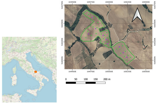
Figure 1.
Left image: Study area (OSM). Right image: Experimental area boundary (green line) of durum wheat cultivars, yield and yield components samplings (green point) and yield quality samplings (purple) (RGB image).
The durum wheat cultivar was Antalis, a medium-cycle variety with a high stay-green and early heading. The spikes are elongated and pyramidal in shape, with white awns. It has a good tillering index, the recommended sowing rate under normal conditions is 300/400 seeds per square meter and 400/450 seeds m−2 in the case of late sowing; therefore, the sowing dose used was 240 kg ha−1. Antalis has a medium–high protein content and a high gluten index and test weight. Seed tanning was performed using a mixture of prothioconazole + fluoxastrobin + tebuconazole. The previous crop was mustard.
Fertilization was carried out with the basic fertilization with a synthetic complex fertilizer, at a dose of 130 Kg ha−1, before the last secondary processing, containing nitrogen, phosphorus, calcium and sulfur plus microelements (N 18, P2O5 20, SO3 14, CaO 4 Fe 0.05, Zn 0.002).
A second fertilization was applied on February 25, during the tillering stage, at a dose of 120 kg ha−1 as the top-dress application of simple mineral fertilizer containing mixed nitrogen salts and sulfur trioxide soluble in water (N 40%, SO3 14%) in granular form. A second, top-dress application with the same mineral fertilizer, at the end of stem elongation, was applied (20 April, during the booting stage); the dose was 150 kg ha−1. A total amount of 131.4 kg ha−1 of nitrogen and 56 kg ha−1 of sulfur were used.
On 29 March, the herbicides iodosulfuron-methyl-sodium and mesosulfuron-methyl were used for post-emergence control of a wide spectrum of grass weeds and broad-leaved weeds on wheat.
On May 14, in the ear emergence, the presence of Septoria tritici blotch disease caused by the fungus Zymoseptoria tritici required the use of fungicidal formulations based on Azoxystrobin (250 g l−1) at a dosage of 0.8 L ha−1, mixed with a fungicidal formulation based on Tebuconazole (250 g kg−1 of product) at a dosage of 400 g ha−1. Harvest was carried out separately for each of the three areas on 26 June 2022. All tractors used in cultivation operations were equipped with precision farming systems such as satellite guidance.
Weather conditions were monitored with a Davis Vantage Pro Wireless Weather Station (Davis Instruments Corp.)
2.2. Methodological Approach
The methodological approach was developed to precisely monitor the wheat plots and to develop assess the agronomic subfield variability by Sentinel-2 NDVI time-series and landscape position. The methodology is divided into three sections (Figure 2). Firstly, subfield areas based on landscape position (topographic features, elevation, slope, aspect) and environmental conditions (meteorological data) were identified.
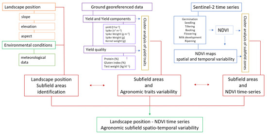
Figure 2.
Flowchart of the proposed method to assess the agronomic subfield variability by Sentinel-2 NDVI time-series and landscape position.
Secondly, ground yield georeferenced data were analyzed according to subfields identified areas by cluster analysis to assess the agronomic subfield variability
Thirdly, Sentinel-2 remote sensing data at different growth stages were preprocessed and the NDVI indices were clustered and analyzed according to landscape position and agronomic subfield variability.
Relationships among landscape position, environmental conditions, phenological stages, yield and yield quality, and subfield areas were analyzed to assess the agronomic subfield variability by Sentinel-2 NDVI time-series and landscape position.
2.2.1. Subfield Areas: Landscape Position and Environmental Conditions
The morphological characteristics made it possible to identify three areas with different exposure, slopes, and microclimate (Figure 3). The three areas share a similar texture to sandy loam soil. Area A (green boundary) is separated from the other areas by the municipal road, whereas area B (yellow boundary) and area C (orange boundary) belong to a single body (Figure 3a). Area A has an area of 2.77 ha, and is a distinct body, totally flat, of a valley nature. Area A has coverage offered by the surrounding hills area. The slope and aspect map of the study area are reported in Figure 3b,c. Area A showed a mean slope of 11%, with 92% of the surface having a slope less than 15% (Figure A1) with a south, south, east aspect. Area B (yellow line) has an area of 1.58 ha and is characterized by a significant average slope of up to 17%. It is exposed to the north-east and influenced by the currents from the Adriatic Sea. This area is also protected from cold winds coming from the northwest, or, rather, by the mountains of Maiella and Gran Sasso, respectively, the second- and the first-highest mountain massifs in the Apennines. Area B showed 65.6% of the surface with a slope of 15–25% (Figure A1). The prevalent aspect was north-east. On the other hand, area C (orange line) has an extension of 4.10 ha and is characterized by a reduced average slope of 14%. It is exposed to the west and northwest, and its microclimate is influenced by the currents coming from the nearby mountain ranges. Areas B and C are divided by the summit ridge with a maximum height of 76 m a.s.l. Area C showed a mean slope of 14%, with 78.4% of the total surface having a slope of 10–20% (Figure A1).
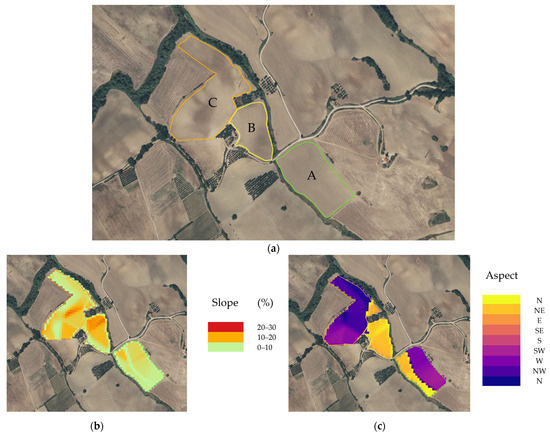
Figure 3.
(a) Map of subfield areas: A (green boundary), area B (yellow boundary), area C (orange boundary). (b) Slope map (%) of the study area. (c) Aspect map of the study area was divided into eight directions from north (0–360).
2.2.2. Ground Yield Data
The crop yield of each area was harvested separately and weighted. Furthermore, 9 samplings for each area were carried out on randomly georeferenced points on an area of 1 m2 each for yield and yield components (Figure 1). The samplings were carried out before the harvest (Zadok’s stage) [35].
Each sample was dried in a ventilated oven at 65 °C until a constant weight was reached, then the grain yield, spike weight, the total number of spikes, and kernel weight were determined.
At harvest, three samples of 500 g for each area were taken randomly to analyze the qualitative characteristics (Figure 1), and the “Crop Scan 1000 B Whole Grain Analyzer” (Next Instruments Pty, Ltd., Canterbury-Bankstown, Condell Park, NSW 2200, Australia) was used to evaluate the protein content, the gluten index, and the test weight.
The CropScan 1000B Whole Grain Analyzer is a near-infrared transmission analyzer designed to measure protein, oil, starch, and moisture in whole grains of wheat, barley, oats, sorghum, canola, corn, soybeans, and more. An optional Test Weight module is available for the CropScan 1000B. The CropScan 1000B uses a diode array spectrometer to scan the wavelength region, 720–1100 nm. Within this region of the NIT spectrum, protein, moisture, oil, and starch absorb NIR energy. Grain is poured into a 500 mL sample cup. A blade is inserted across the grain and the excess grain is poured out. The blade is removed from the cup and the 500 mL of grain is poured into the sample hopper. The grain is metered through the optical chamber where the NIT spectra are collected and stored in memory. An average of between 10 and 30 spectra are used to compute the percentage of protein, oil, and moisture. The grain falls into the sample cup which is located on a load cell. The weight of the 500 mL of grain is recorded and displayed along with the protein, oil, and moisture.
2.2.3. Sentinel-2 Data
The European Space Agency (ESA) launched the Copernicus Programme in 2014 to improve forest status surveillance, land-use monitoring, and disaster management capacity by launching a series of Sentinel satellites [36]. Sentinel-2, which consists of two optical remote sensing satellites, can provide multispectral data (13 bands) with a relatively high spatial resolution (10 m, 20 m, and 60 m). Sentinel-2A was successfully launched in late June 2015, and Sentinel-2B was launched in March 2017. The revisit period was shortened to only 5 days when the two satellites operate simultaneously, which greatly enhanced the Earth’s observation ability when compared with the existing satellites. In the present study, Level 2A (radiometrically and atmospherically corrected) bottom-of-atmosphere (BOA) reflectance products provided by ESA were used. The screening criteria for downloading were the durum wheat phenological stage and zero or close to zero (<10%) cloud cover. A total of 7 cloud-free Sentinel-2 (A and B) images from 22 January 2021 to 21 June 2022 (Table 1) met these criteria and were downloaded from ESA’s Copernicus Open Access Hub (https://scihub.copernicus.eu/ (accessed on 1 September 2022). All images were resampled at 10 m pixel size using the SNAP-ESA Sentinels Application Platform v.6.0.4 (http://step.esa.int (accessed on 30 September 2022)) free open-source software. Afterwards, data extraction was performed for the pixels of the studied sites.

Table 1.
Sentinel-2 images data acquisition period, durum wheat crop growth stage (Zadok’s scale), and day after showing (DAS).
The NDVI time-series were computed from the 10 m spatial resolution red (ρRED) and near-infrared (ρNIR) spectral bands from Sentinel-2 images, as follows [37]:
NDVI = (ρNIR − ρRED)/(ρNIR + ρRED)
The results were elaborated in Quantum GIS (QGIS) software version 3.2.3 (QGIS Development Team, 2009. QGIS Geographic Information System. Open Source Geospatial Foundation. URL http://qgis.org, (accessed on 30 September 2022)), provided by the Open Source Geospatial Foundation (OSGeo). All calculations were performed using the QGIS raster calculator; furthermore, Point Sampling Tool was used to extract raster data values to each georeferenced point.
The Sentinel-2 spectral bands No. 4 (red) and No. 8 (NIR) with a spatial resolution of 10 m were used for NDVI calculations. The red band, with a central wavelength (nm) of 665 and a bandwidth of 30, and the NIR band No. 8, with a central wavelength (nm) of 842 and a bandwidth of 115, were elaborated in the Quantum GIS (QGIS) software provided by the Open Source Geospatial Foundation (OSGeo). The NDVI of the selected images was calculated using the Raster Calculator tool available in the QGIS raster menu. In addition, the Point Sampling tool was used to extract raster data values for each georeferenced point. The NDVI images were elaborated and analyzed. Unsupervised image classification using clustering algorithms was used to categorize the NDVI images.
The Semi-Automatic Classification Plugin and the k-means cluster method were used [38]. The Semi-Automatic Classification Plugin aims to provide a complete suite of tools for processing remote sensing data, easing the phases related to the download, the preprocessing of images, and the post-processing of classifications, with built-in algorithms developed in Python and third-party algorithms for specific functions (e.g., Sentinel-2 preprocessing through ESA SNAP) [39]. The algorithm splits clusters with too-high variability of spectral signatures based on the standard deviation, since many spectral signatures can be defined in the initial preprocessing phase to capture the number of clusters expected in the image. Hence, the initial parameters provided by the users in SCP implementation are C = number of desired clusters, Nmin = minimum number of pixels for a cluster, σt = maximum standard deviation threshold for splitting, and Dt = distance threshold for merging. The algorithm proceeds with the iterative procedure by calculating Euclidean distance (minimum distance algorithm), and the pixels are assigned to produce clusters according to the most similar spectral signature. With several trials of clustering, where the number of classes = 3, maximum standard deviation = 0.02, and minimum class size in pixel = 10, 20 iterations applying minimum distance seed signatures at a distance threshold of 0.01 were used to produce the NDVI image cluster.
2.3. Statistical Analysis
Data were analyzed by one-way analysis ANOVA with a significance level of p < 0.05. Pairs of means were compared using the Tukey HSD test. All statistical analyses were performed using Origin Pro software (OriginLab Corporation, Northampton, MA, USA).
3. Results
3.1. Meteorological Data
The amount of rain that fell in October, November, and December 2021 was 366 mm (more than three times the previous year’s rainfall and the same amount of total rainfall per year). A total of 159.2 mm of rain was recorded from sowing to harvest (Table 2). The temperature ranged from a minimum of −1.2 °C on 12 March to 37.5 °C on 20 June. The wettest month was March, with 52.2 mm of precipitation and six events, and the driest month was April. During the winter months, cold winds were recorded, and in the spring months, the warmer air came mostly from the southern slopes.
Table 2.
Meteorological data, minimum and maximum temperature (°C), rain (mm), number of rain events, max rain amount per event (mm), and wind max (km h−1) collected by the meteorological station in the field experiment.
3.2. Yield Traits and Landscape Position
At harvest, the entire field had a grain yield of 5.47 t ha−1 with a number of 386 ears per square meter. The mean ear weight was 2.07 g with a grain weight of 1.42 g and a percentage of filled grains of 68.6%. Protein content reached 14.4% with a gluten index of 11.5%. The test weight was 87.4 kg hl−1. The field showed great spatial variability, and the yield ranged from 3.91 t ha−1 to 7.17 t ha−1, with a wide range of ears per square meter (324 to 540) and a percentage of filled grains between 62% and 78.5%. Protein content ranged from 13.9% to 14.9%, gluten content from 10.9% to 12.2%, and test weight from 85.0 to 90.9.
3.3. NDVI Derived from Sentinel-2 Spatial and Temporal Variability
NDVI derived from Sentinel-2 images at seven different growth stages, from emergence to ripening, was recorded and analyzed (Figure 4). The NDVI at germination was higher than at seedling due to soil reflectance; therefore, the germination NDVI data were not further used for analysis. Furthermore, data at ripening cannot provide indications of crop spatial variability due to the senescence of the plant. The lower NDVI mean value of 0.16 was recorded at the seeding growth stage (11 February), and the highest value was recorded at the booting and flowering stages, with NDVI mean values of 0.55 and 0.54, respectively. The highest variability value of NDVI was recorded at tillering stage followed by the milk development and booting stages, respectively.
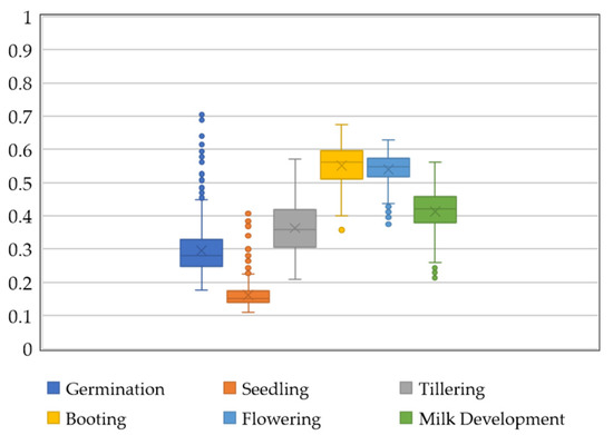
Figure 4.
Box plot of NDVI data collected at germination, seedling, tillering, booting, flowering, and milk development growth stages. The minimum, maximum, first quartile (Q1 or 25th percentile), third quartile (Q3 or 75th percentile), and median values are reported. Values that lie in both extremes of data were reported as points (outliers).
The NDVI maps (Figure 5) showed the main variability at tillering stage and milk development stage, with the highest values in the flat area and low values in the center of the field. Visual examination showed no spatial difference between germination and seedling growth stages.
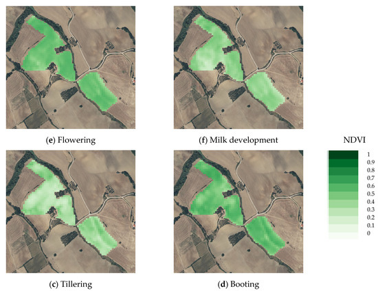
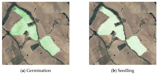
Figure 5.
NDVI maps (0–1) derived from the Sentinel-2 images at (a) germination, (b) seedling, (c) tillering, (d) booting, (e) flowering, and (f) milk development Zadok’s stages.
3.4. Agronomic Traits and Landscape Position
Due to the different locations of the fields in the landscape and topographic features (morphology, altitude, exposure), the crop area data for the three areas were analyzed separately.
Yield sampling data in area A was 6.77 t ha−1, followed by area B with 6.05 t ha−1, and finally area C with a mean value of 4.38 t ha−1 and a significant yield difference related to subareas A and B (Table 3). The subfield with the higher number of ears per square meter was subfield B, with an average number of ears per square meter of 477, significantly higher than subfield A (399 ears per square meter) and subfield C (343 ears per square meter). Ear weight and kernel weight were higher in subfield A than in subfields B and C. No significant differences were found between subfields B and C.
Table 3.
Subfields A, B, and C yield (t ha−1), spike (n° m−2), spike weight (g m−2), spike weight (g), kernel weight (g) data, standard deviation (SD), ANOVA one-way, degrees of freedom (df), sum of square (SS), mean square (MS), F-value, and p-value. For each mean effect, values in a column followed by the same letter are not significantly different at p ≤ 0.05, different letter are significantly different at p ≤ 0.05 as determined by the Fisher test.
Mechanical harvest data per unit area evaluated after threshing showed an average of 6.3 t ha−1 for area A, 5.6 t ha−1 for area B, and 4.1 t ha−1 for area C. Harvest data showed a mean yield value lower than georeferenced data sampling of about 5–7%.
The protein content, gluten index (%), and test weight (kg hl−1) of each area were evaluated (Table 4). The protein content was higher in area A (14.7%) and ranged from 14.1 to 14.2 for subfields B and C, respectively. Differences in the gluten index value of subfield A were recorded, and subfields B and C showed an 11.2 gluten value. The test weight was higher for subfield B relative to subfields A and C.
Table 4.
Subfields A, B, and C protein (%), gluten index (%), test weight (kg hl−1) data, standard deviation (SD), ANOVA one-way, degrees of freedom (df), sum of square (SS), mean square (MS), F-value, and p-value. For each mean effect, values in a column followed by the same letter are not significantly different at p ≤ 0.05, different letter are significantly different at p ≤ 0.05 as determined by the Fisher test.
3.5. NDVI Time-Series and Landscape Position
NDVI data obtained from Sentinel-2 imagery at the time of seedling, tillering, booting, flowering, and milk development were clustered by k-means cluster analysis using the QGIS Semi-Automatic Classification Plugin (Figure 6). At the seedling stage, no differences among the three areas were recorded. The k-means analysis of the NDVI data from the Sentinel-2 images from tillering to milk development resulted in three distinct clusters. The mean value of each area and the cluster data for each growth stage were analyzed. At tillering stage, area A showed a high mean NDVI value (0.39) (Figure A2) with 85% of the surface in cluster 1 and 2 (high 40% and medium 45% NDVI value). The areas B and C showed NDVI mean values of 0.34 and 0.35, respectively (Figure A2). Area B showed 51% of surface in cluster 2 (medium value) and 40% in cluster 3 (low value), and area C showed 48% of the surface in cluster 3 (low value) and 28% in cluster 2 (medium value).
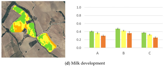
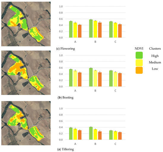
Figure 6.
NDVI derived from the Sentinel-2 images and clusters’ map (sx) and NDVI data of combined cluster and landscape position (dx) with high, medium, and low subfield areas at (a) tillering, (b) booting, (c) flowering, and (d) milk development Zadok’s stages.
The map with the surfaces with the three NDVI clusters (Figure 6a) at tillering stage highlight the big area with high and medium value for subfield A, subfield B with almost all the surfaces in the medium and low NDVI clusters, and subfield C with the central surface in the middle and low NDVI clusters. The NDVI cluster data and the landscape position showed a difference among the NDVI value of each subfield area. The higher mean value for the NDVI was high for area B, and NDVI was medium and low for area A. Area C showed lower NDVI values (Table A1).
At the booting stage, the NDVI mean value of the three subfield areas ranged from 0.54 (area B) to 0.56 (area A) with a rebalancing of the resulting clusters (Figure A2). The surface with a high NDVI value was about 48% for area A, 40% for area B, and 43% for area C. The surfaces with low NDVI values were lower than 25% for all the subfield area.
At booting (Figure 6a), a reduction of the areas identified at tillering with low values and a rebalancing with the other value classes was observed. The NDVI cluster data and the landscape position showed a higher mean value for the NDVI high for area B, and NDVI medium and low for areas A and B.
At the flowering stage (Figure 6c), the NDVI mean values ranged from 0.53 (area A) to 0.56 (area B), with a different distribution of the subfield areas (Figure A2). Area A showed 40% of the surface with a high NDVI value and 46% of the surface with a medium NDVI value. Area B showed 67% of the surface with a high NDVI value and 29% with a medium value. Area C showed 48% of the surface with a high value and 41% with a medium value. The lower NDVI values at the flowering stage were in the outer part of field A (Figure 5c), at the top and in the most downstream part of field B, and in the outermost part towards the west of field C. The area with average values occupied a large surface both in area A and in area C. The NDVI cluster data and the landscape position showed a higher mean value for the NDVI high, medium, and low for the area B.
At the milk development stage (Figure 6d), the NDVI mean value of the three subfield areas ranged from 0.41 (areas A and C) to 0.43 (area B) (Figure A2). The surface with a high NDVI value was about 35% for area A, 52% for area B, and 43% for Area C. The surface with low NDVI values was lower than 15% for area A, 6% for area B, and 25% for area C. At the booting stage, an increase of low areas identified at tillering in areas C and A was observed. The NDVI cluster data and the landscape position showed a higher mean value for the NDVI high, medium, and low for the area B.
4. Discussion
Improving the resilience of agricultural production to weather variability and climate change requires a better understanding of the underlying processes that lead to weather-related crop stress and yield loss [29]. Temperature and precipitation trends in the Mediterranean region have been critical for durum wheat due to climate change [21]. In addition, the location of the landscape at the farm level mediates the microenvironment to which crops are exposed and which can significantly mitigate or exacerbate weather-related crop stress.
The NDVI derived from Sentinel-2 imagery can be used to define homogeneous areas associated with agronomic characteristics [40]; however, a more comprehensive approach may be needed to improve the efficiency of the management strategy at the farm level.
The open field area of 8.45 ha was analyzed. Despite the sowing delays, frequent winter frosts, and prolonged spring drought, excellent results in terms of grain yield and quality were obtained in all the studied areas. The mean yield value (5.47 t ha−1) was 12% lower than the values found by Tavoletti and Merletti [41] on the same variety under similar environmental conditions.
However, an important spatial variability was found, with double production values in some areas compared to others and differences in proteins of up to 4%. The analysis of yield components, NDVI cluster map, and land position provided useful information to characterize spatial variability and agronomic needs.
The whole field has an irregular shape and can be divided into three areas (A, B, and C) with different topographic characteristics (morphology, altitude, and aspect).
Subfield A performed the best in terms of grain yield, with a mean yield value 10% higher than subfield B and 35% higher than subfield C. The difference in yield is mainly due to good tillering, and the higher weight of ears and grains per ear than in areas B and C. Quality parameters showed the same trend, with a higher protein content for area A of +3% and +3.8% and a gluten index +5.5% and +7% higher than in areas B and C. Results are in agreement with Basso et al. [42], who found that the spatial location of the highest yield measured corresponded with the location where the highest protein content was also measured. Field A is a distinct, almost completely separated body with valley character, characterized by a higher and more permanent soil moisture value than the other two areas, an important attribute in the drought period which can be a limiting factor in particularly rainy years; in addition, the morphology of the subfield protects the crop from winter frosts and improves water availability in spring, an important factor, especially in the absence of irrigation and in the context of climate change. McKinion et al. [30] found more productive results in flat areas with the same characteristics as area A than in sloping areas, especially in dry seasons. The main reason is that these areas are typified by receiving more water from drainage from the surrounding higher elevations.
As expected, comparison of the NDVI with yield values reveals a significant positive linear relationship in terms of both correlations and timing, and results are in line with findings by many authors [11,40,43,44]. The NDVI derived from the Sentinel-2 cluster map data confirms the higher values of subclusters with high, medium, and low values, respectively, and provides useful information about the lower cluster subfields in the marginal areas of the field that are more exposed to water flow in the spring. The NDVI derived from the Sentinel-2 cluster map results were in accordance with data found by Marino et al. [45]. The yield value of area A was 9% higher than Tavoletti and Merletti [41], highlighting, in years with drought springs and summers, important advantages compared to other areas.
Subfield B had a mean yield value of 6 t ha−1 that was not significantly different from subfield A, although the yield component showed a completely different trend. Area B is characterized by a considerable average slope and different microclimatic conditions due to the slope and location. Area B is protected from the cold winter winds and is moderated by the influence of the Adriatic Sea. In the spring, in the phase of soil cultivation, less waterlogging was recorded, which led to a significant increase in the number of ears per square meter: +16.3% and +28% for areas A and C, respectively. The higher NDVI value at booting confirms this finding. In contrast, in areas exposed by the slope to more direct sunlight, in the summer, water drains away from these areas due to the slope, therefore, less water is available to the crops [30]. For this reason, area B suffered more from drought in summer, with lower ear weight and grain weight per spike than area A and comparable to area C. This information matches what is evidenced by the NDVI values, which showed in area B a reduction in the highest cluster area and improvement in the medium cluster area values passing from flowering to the milk development stage. In area B, the “stay-green” effect of the variety might have affected grain filling, suggesting that it would have been wise to reduce investment in seed per hectare or, if possible, to apply emergency irrigation in the summer season to reduce competition for water resources and thus hope for greater filling of the ears. Nagarajan et al. [46] found that grain filling and partitioning of assimilates to developing grains are affected by post-anthesis water deficit. This area can be described as being a high slope, with a northeast exposure generally having less water availability in summer and being exposed to more direct sunlight. This information can be useful above all for the planning of the following years; in fact, as also reported by Christopher et al. [47], a decrease in stay-green, as a response, for example, to water stress, may affect grain yield through an accelerated reduction of photosynthetic assimilates during the grain filling, which might be too late for reasoned management (e.g., additional irrigation or top-dressing fertilization). Furthermore, according to Basso et al. [41], the highest rainfall that occurred in the winter growing season did not force the roots to grow deeper into the soil, so when rainfall decreased during anthesis, the shallow rooting system was not able to meet the evapotranspiration demand with the limited rainfall that occurred in spring. Heat stress during grain filling and drought during the stem elongation and grain-filling stages were identified as critical environmental factors [48]. Furthermore, the NDVI value had the lowest values (cluster 3) in the central area of area B, characterized by the highest slopes (FAT MAP), confirming the results of [42]. Comparing the three areas, area B has always had very high NDVI values, both for high, medium, and low NDVI clusters, compared to areas A and C, as expected.
Area C was more exposed to cold winter winds and frost risk. The cold airflow from the Balkans and the northeast (bora) wind blows less often, most commonly occurring during the winter months and affecting the temperatures [49]. The lowest average yield (4.1 t ha−1) of harvested grain was observed, although qualitative parameters remained anchored at good values. Of the three areas, area C has the most important areas included in NDVI cluster 3 and cluster 2 at tillering, and the widest air with low NDVI values at the milk stage (21%), highlighting a certain relationship between production and NDVI which, however, has been underestimated. The use of a variety more resistant to thermal stress from the cold would have responded better to environmental adversities and could improve grain yield. The results confirm what was found by Basso et al. [42], which was that in the Mediterranean context, aspect, altitude, and slope are directly linked with wheat grain yield and that rainfall is a major limiting factor for wheat yields [50,51]. We agree with La Gouis et al. [24] that adaptation to climate change will pass through a combination of changes in agricultural practices (modifying the date of sowing, piloting at best irrigation, and fertilization through efficient decision-making tools, developing conservation agriculture and agro-forestry) maintaining the genetic progress.
5. Conclusions
Significant advancements in the application of geospatial technologies, remotely sensed images, and more precise ground data monitors have allowed for improving the information on spatial and temporal variations of crop yields occurring in the field. Understanding wheat grain yield variability within a field is central to applying precision farming management practices and improving environmental, agricultural, and socioeconomic sustainability. In this article, the performances of NDVI derived from Sentinel-2 time-series images and landscape position were analyzed to define the most effective agronomic parameters for within-field grain yield variability mapping. Three different areas for landscape position, microclimate conditions, and topographic features were identified. The variability in space and time affected the yield and quality of data. The most important factors that determined the yield variability in the winter period were the position and exposure of the subfield due to temperatures and winds, and the slope due to excess water. In particular, sloping fields with exposures sheltered from cold winds saw a greater number of spikes per square meter than other areas. In the summer period, considering the scarcity of rain, the areas with the best characteristics were those with the greatest capacity to store water or to receive water from the surrounding areas; furthermore, the areas exposed to the prevailing colder winds were the least productive. The NDVI index derived from Sentinel-2 and the cluster analysis positively identified areas with different characteristics between and within areas, providing valid indications during the growth cycle. The agronomic management strategies in the areas identified within the same clusters, and in particular those with medium and low NDVI values, however, require completely different agronomic management strategies. In the Mediterranean context, aspect, altitude, and slope are directly linked with wheat grain yield and quality, and rainfall is a major limiting factor for wheat yield, although in the analysis of satellite data they are often little used. In a hilly environment and climate change scenario, NDVI time-series data derived by Sentinel-2 images can be more effective if merged with landscape position, topographic features, and microclimate data. Sentinel-2 data and landscape position analysis can be used to identify high, medium, and low NDVI values differentiated by subfield areas and associated with specific agronomic traits to improve agronomic site-specific management.
Funding
This research received no external funding.
Data Availability Statement
The data presented in this study are available on request from the corresponding author. The data are not publicly available due to privacy.
Acknowledgments
We would like to express our special thanks to Marco Berchicci who helped with the farm activities.
Conflicts of Interest
The authors declare no conflict of interest.
Appendix A

Figure A1.
Slope surface area (class of slope, %) of the subfield area A (a), area B (b), area C (c), and of the experimental field (d).

Figure A2.
Box plot of the NDVI data variability in each area (A, B, C) at different growth stages (1—seedling; 2—tillering, 4—booting, 6—flowering, and 7—milk development).
Table A1.
Analysis of NDVI variance of clusters identified by k-means cluster method at tillering, booting, flowering, and milk development stages related to Figure 6 data.
Table A1.
Analysis of NDVI variance of clusters identified by k-means cluster method at tillering, booting, flowering, and milk development stages related to Figure 6 data.
| Between SS | df | Within SS | DF | F | Signif. p | ||
|---|---|---|---|---|---|---|---|
| A | 0.139 | 2 | 0.028 | 137 | 341.6 | 0.00 | |
| Tillering | B | 0.387 | 2 | 0.093 | 137 | 284.1 | 0.00 |
| C | 0.057 | 2 | 0.010 | 137 | 381.8 | 0.00 | |
| A | 0.219 | 2 | 0.031 | 137 | 479.6 | 0.00 | |
| Booting | B | 0.429 | 2 | 0.065 | 137 | 451.3 | 0.00 |
| C | 0.151 | 2 | 0.025 | 137 | 404.6 | 0.00 | |
| A | 0.242 | 2 | 0.032 | 137 | 526.5 | 0.00 | |
| Flowering | B | 0.166 | 2 | 0.036 | 137 | 320.7 | 0.00 |
| C | 0.150 | 2 | 0.019 | 137 | 535.9 | 0.00 | |
| A | 0.241 | 2 | 0.028 | 137 | 597.5 | 0.00 | |
| Milk development | B | 0.241 | 2 | 0.060 | 137 | 276.7 | 0.00 |
| C | 0.297 | 2 | 0.037 | 137 | 547.4 | 0.00 |
References
- Basso, B.; Cammarano, D.; Carfagna, E. Review of crop yield forecasting methods and early warning systems. In Proceedings of the First Meeting of the Scientific Advisory Committee of the Global Strategy to Improve agricultural and Rural Statistics, Rome, Italy, 18–19 July 2013; FAO Headquarters: Rome, Italy, 2013; Volume 18, p. 19. [Google Scholar]
- Miao, Y.; Mulla, D.J.; Robert, P.C. Identifying important factors influencing corn yield and grain quality variability using artificial neural networks. Precis. Agric. 2006, 7, 117–135. [Google Scholar] [CrossRef]
- Kravchenko, A.N.; Robertson, G.P.; Thelen, K.D.; Harwood, R.R. Management, Topographical, and Weather Effects on Spatial Variability of Crop Grain Yields. Agron. J. 2005, 97, 514–523. [Google Scholar] [CrossRef]
- Marino, S.; Alvino, A. Detection of Spatial and Temporal Variability of Wheat Cultivars by High-Resolution Vegetation Indices. Agronomy 2019, 9, 226. [Google Scholar] [CrossRef]
- Hunt, M.L.; Blackburn, G.A.; Carrasco, L.; Redhead, J.W.; Rowland, C.S. High resolution wheat yield mapping using Sentinel-2. Remote Sens. Environ. 2019, 233, 111410. [Google Scholar] [CrossRef]
- Cavalaris, C.; Megoudi, S.; Maxouri, M.; Anatolitis, K.; Sifakis, M.; Levizou, E.; Kyparissis, A. Modeling of Durum Wheat Yield Based on Sentinel-2 Imagery. Agronomy 2021, 11, 1486. [Google Scholar] [CrossRef]
- Padilla, F.L.M.; Maas, S.J.; González-Dugo, M.P.; Mansilla, F.; Rajan, N.; Gavilán, P.; Domínguez, J. Monitoring Regional Wheat Yield in Southern Spain Using the GRAMI Model and Satellite Imagery. Field Crops Res. 2012, 130, 145–154. [Google Scholar] [CrossRef]
- Silvestro, P.C.; Pignatti, S.; Pascucci, S.; Yang, H.; Li, Z.; Yang, G.; Huang, W.; Casa, R. Estimating Wheat Yield in China at the Field and District Scale from the Assimilation of Satellite Data into the Aquacrop and Simple Algorithm for Yield (SAFY) Models. Remote Sens. 2017, 9, 509. [Google Scholar] [CrossRef]
- Gaso, D.V.; Berger, A.G.; Ciganda, V.S. Predicting Wheat Grain Yield and Spatial Variability at Field Scale Using a Simple Regression or a Crop Model in Conjunction with Landsat Images. Comput. Electron. Agric. 2019, 159, 75–83. [Google Scholar] [CrossRef]
- Bebie, M.; Cavalaris, C.; Kyparissis, A. Assessing Durum Wheat Yield through Sentinel-2 Imagery: A Machine Learning Approach. Remote Sens. 2022, 14, 3880. [Google Scholar] [CrossRef]
- Toscano, P.; Castrignanò, A.; Di Gennaro, S.F.; Vonella, A.V.; Ventrella, D.; Matese, A. A Precision Agriculture Approach for Durum Wheat Yield Assessment Using Remote Sensing Data and Yield Mapping. Agronomy 2019, 9, 437. [Google Scholar] [CrossRef]
- Fieuzal, R.; Bustillo, V.; Collado, D.; Dedieu, G. Combined Use of Multi-Temporal Landsat-8 and Sentinel-2 Images for Wheat Yield Estimates at the Intra-Plot Spatial Scale. Agronomy 2020, 10, 327. [Google Scholar] [CrossRef]
- Skakun, S.; Vermote, E.; Franch, B.; Roger, J.-C.; Kussul, N.; Ju, J.; Masek, J. Winter Wheat Yield assessment from Landsat 8 and Sentinel-2 Data: Incorporating Surface Reflectance, Through Phenological Fitting, into Regression Yield Models. Remote Sens. 2019, 11, 1768. [Google Scholar] [CrossRef]
- Segarra, J.; Araus, J.L.; Kefauver, S.C. Farming and Earth Observation: Sentinel-2 data to estimate within-field wheat grain yield. Int. J. Appl. Earth Obs. Geoinf. 2022, 107, 102697. [Google Scholar] [CrossRef]
- Marino, S.; Alvino, A. Detection of homogeneous wheat areas using multi-temporal UAS images and ground truth data analyzed by cluster analysis. Eur. J. Remote Sens. 2018, 51, 266–275. [Google Scholar] [CrossRef]
- Kumhálová, J.; Moudrý, V. Topographical characteristics for precision agriculture in conditions of the Czech Republic. Appl. Geogr. 2014, 50, 90–98. [Google Scholar] [CrossRef]
- Liu, W.; Ye, T.; Jägermeyr, J.; Müller, C.; Chen, S.; Liu, X.; Shi, P. Future climate change significantly alters interannual wheat yield variability over half of harvested areas. Environ. Res. Lett. 2021, 16, 094045. [Google Scholar] [CrossRef]
- Appiotti, F.; Krželj, M.; Russo, A.; Ferretti, M.; Bastianini, M.; Marincioni, F. A multidisciplinary study on the effects of climate change in the northern Adriatic Sea and the Marche region (central Italy). Reg Environ. Change 2014, 14, 2007–2024. [Google Scholar] [CrossRef]
- Porter, J.R.; Gawith, M. Temperatures and the growth and development of wheat: A review. Eur. J. Agron. 1999, 10, 23–36. [Google Scholar] [CrossRef]
- Ottman, M.J.; Kimball, B.A.; White, J.W.; Wall, G.W. Wheat growth response to increased temperature from varied planting dates and supplemental infrared heating. Agron. J. 2012, 104, 7–16. [Google Scholar] [CrossRef]
- Reidsma, P.; Ewert, F.; Lansinkc, A.O.; Leemansd, R. Adaptation to climate change and climate variability in European agriculture: The importance of farm level responses Eur. J. Agron. 2010, 32, 91–102. [Google Scholar] [CrossRef]
- Zhao, C.; Liu, B.; Piao, S.; Wang, X.; Lobell, D.B.; Huang, Y.; Huang, M.; Yao, Y.; Bassu, S.; Ciais, P. Temperature increase reduces global yields of major crops in four independent estimates. Proc. Natl. Acad. Sci. USA 2017, 114, 9326–9331. [Google Scholar] [CrossRef] [PubMed]
- Porter, J. Rising temperatures are likely to reduce crop yields. Nature 2005, 436, 174. [Google Scholar] [CrossRef] [PubMed]
- Le Gouis, J.; Oury, F.-X.; Charmet, G. How changes in climate and agricultural practices influenced wheat production in Western Europe. J. Cereal Sci. 2020, 93, 102960. [Google Scholar] [CrossRef]
- Barlow, K.; Christy, B.; O’leary, G.; Riffkin, P.; Nuttall, J. Simulating the impact of extreme heat and frost events on wheat crop production: A review. Field Crops Res. 2015, 171, 109–119. [Google Scholar] [CrossRef]
- Salehi-Lisar, S.Y.; Bakhshayeshan-Agdam, H. Drought stress in plants: Causes, consequences, and tolerance. In Drought Stress Tolerance in Plants; Springer: Berlin/Heidelberg, Germany, 2016; Volume 1, pp. 1–16. [Google Scholar]
- Maestrini, B.; Basso, B. Drivers of within-field spatial and temporal variability of crop yield across the US Midwest. Sci. Rep. 2018, 8, 14833. [Google Scholar] [CrossRef]
- Maestrini, B.; Basso, B. Predicting spatial patterns of within-field crop yield variability. Field Crop. Res. 2018, 219, 106–112. [Google Scholar] [CrossRef]
- Martinez-Feria, R.A.; Basso, B. Unstable crop yields reveal opportunities for site-specific adaptations to climate variability. Sci. Rep. 2020, 10, 2885. [Google Scholar] [CrossRef]
- McKinion, J.M.; Willers, J.L.; Jenkins, J.N. Spatial analyses to evaluate multi-crop yield stability for a field. Comput. Electron. Agric. 2010, 70, 187–198. [Google Scholar] [CrossRef]
- Segarra, J.; González-Torralba, J.; Aranjuelo, Í.; Araus, J.L.; Kefauver, S.C. Estimating Wheat Grain Yield Using Sentinel-2 Imagery and Exploring Topographic Features and Rainfall Effects on Wheat Performance in Navarre, Spain. Remote Sens. 2020, 12, 2278. [Google Scholar] [CrossRef]
- Romano, E.; Bergonzoli, S.; Pecorella, I.; Bisaglia, C.; De Vita, P. Methodology for the Definition of Durum Wheat Yield Homogeneous Zones by Using Satellite Spectral Indices. Remote Sens. 2021, 13, 2036. [Google Scholar] [CrossRef]
- Ahmad, U.; Nasirahmadi, A.; Hensel, O.; Marino, S. Technology and Data Fusion Methods to Enhance Site-Specific Crop Monitoring. Agronomy 2022, 12, 555. [Google Scholar] [CrossRef]
- Aucelli, P.P.C.; Fortini, P.; Rosskopf, C.M.; Scorpio, V.; Viscosi, V. Effects of recent channel adjustments on riparian vegetation: Some examples from Molise region (Central Italy). Geogr. Fis. Din. Quat. 2011, 34, 161–173. Geogr. Fis. Din. Quat. 2011, 34, 161–173. [Google Scholar]
- Zadoks, J.C.; Chang, T.T.; Konzak, C.F. A decimal code for the growth stages of cereals. Weed Res. 1974, 14, 415–421. [Google Scholar] [CrossRef]
- Mecklenburg, S.; Drusch, M.; Kerr, Y.H.; Martin-Neira, M.; Delwart, S.; Buenadicha, G.; Reul, N.; Daganzo-Eusebio, E.; Oliva, R.; Crapolicchio, R. ESA’s soil moisture and ocean salinity mission: Mission performance and operations. IEEE Trans. Geosci. Remote Sens. 2012, 50, 1354–1366. [Google Scholar] [CrossRef]
- Rouse, J.W.; Hass, R.H.; Schell, J.A.; Deering, D.W. Monitoring vegetation systems in the great plains with ERTS. In Proceedings of the Third Earth Resources Technology Satellite-1 Symposium: The Proceedings of a Symposium Held by Goddard Space Flight Center, Washington, DC, USA, 10–14 December 1973; Volume 1, pp. 309–317. [Google Scholar]
- Tempa, K.; Aryal, K.R. Semi-automatic classification for rapid delineation of the geohazard-prone areas using Sentinel-2 satellite imagery. SN Appl. Sci. 2022, 4, 141. [Google Scholar] [CrossRef]
- Congedo, L. Semi-Automatic Classification Plugin: A Python tool for the download and processing of remote sensing images in QGIS. J. Open Source Softw. 2021, 6, 3172. [Google Scholar] [CrossRef]
- Marino, S.; Alvino, A. Vegetation Indices Data Clustering for Dynamic Monitoring and Classification of Wheat Yield Crop Traits. Remote Sens. 2021, 13, 541. [Google Scholar] [CrossRef]
- Tavoletti, S.; Merletti, A. A comprehensive approach to evaluate durum wheat–faba bean mixed crop performance. Front. Plant Sci. 2022, 13, 733116. [Google Scholar] [CrossRef]
- Basso, B.; Cammarano, D.; Chen, D.; Cafiero, G.; Amato, M.; Bitella, G.; Rossi, R.; Basso, F. Landscape Position and Precipitation Effects on Spatial Variability of Wheat Yield and Grain Protein in Southern Italy. J. Agron. Crop. Sci. 2009, 195, 301–312. [Google Scholar] [CrossRef]
- Mahey, R.K.; Singh, R.; Sidhu, S.S.; Narang, R.S. The use of remote sensing to assess the effects of water stress on wheat. Exp. Agric. 1991, 27, 423–429. [Google Scholar] [CrossRef]
- Freeman, K.W.; Raun, W.R.; Johnson, G.V.; Mullen, R.W.; Stone, M.L.; Solie, J.B. Late-season prediction of wheat grain yield and grain protein. Commun. Soil Sci. Plant Anal. 2003, 34, 1837–1852. [Google Scholar] [CrossRef]
- Marino, S.; Alvino, A. Agronomic Traits Analysis of Ten Winter Wheat Cultivars Clustered by UAV-Derived Vegetation Indices. Remote Sens. 2020, 12, 249. [Google Scholar] [CrossRef]
- Nagarajan, S.; Rane, J.; Maheswari, M.; Gambhir, P.N. Effect of post-anthesis water stress on accumulation of dry matter, carbon and nitrogen and their partitioning in wheat varieties differing in drought tolerance. J. Agron. Crop Sci. 1999, 183, 129–136. [Google Scholar] [CrossRef]
- Christopher, J.T.; Christopher, M.J.; Borrell, A.K.; Fletcher, S.; Chenu, K. Staygreen traits to improve wheat adaptation in well-watered and water-limited environments. J. Exp. Bot. 2016, 67, 5159–5172. [Google Scholar] [CrossRef] [PubMed]
- Brisson, N.; Gate, P.; Gouache, D.; Charmet, G.; Oury, F.X.; Huard, F. Why are wheat yields stagnating in Europe? A comprehensive data analysis for France. Field Crop. Res. 2010, 119, 201–212. [Google Scholar] [CrossRef]
- Bonacci, O.; Vrsalović, A. Differences in Air and Sea Surface Temperatures in the Northern and Southern Part of the Adriatic Sea. Atmosphere 2022, 13, 1158. [Google Scholar] [CrossRef]
- Basso, B.; Fiorentino, C.; Cammarano, D.; Cafiero, G.; Dardanelli, J. Analysis of rainfall distribution on spatial and temporal patterns of wheat yield in Mediterranean environment. Eur. J. Agron. 2012, 41, 52–65. [Google Scholar] [CrossRef]
- Ferrara, R.M.; Trevisiol, P.; Acutis, M.; Rana, G.; Richter, G.; Baggaley, N. Topographic impacts on wheat yields under climate change: Two contrasted case studies in Europe. Theor. Appl. Clim. 2009, 99, 53–65. [Google Scholar] [CrossRef]
Disclaimer/Publisher’s Note: The statements, opinions and data contained in all publications are solely those of the individual author(s) and contributor(s) and not of MDPI and/or the editor(s). MDPI and/or the editor(s) disclaim responsibility for any injury to people or property resulting from any ideas, methods, instructions or products referred to in the content. |
© 2022 by the author. Licensee MDPI, Basel, Switzerland. This article is an open access article distributed under the terms and conditions of the Creative Commons Attribution (CC BY) license (https://creativecommons.org/licenses/by/4.0/).