Article

Historical Changes in Agricultural Systems and the Current Greenhouse Gas Emissions in Southern Chile

by
Francisca Meneses
1,
Nicole Montenegro
2,
Constanza Schapheer
1 and
Jorge F. Perez-Quezada
1,3,4,*
1
Department of Environmental Science and Renewable Natural Resources, University of Chile, Santiago 8820808, Chile
2
Laboratoire des Sciences du Climat et de l’Environnement, LSCE-IPSL (CEA-CNRS-UVSQ), Université Paris-Saclay, 91191 Gif-sur-Yvette, France
3
Institute of Ecology and Biodiversity (IEB), Victoria 631, Concepción 4030000, Chile
4
Cape Horn International Center, CHIC, O’Higgins N°310, Cabo de Hornos 6350000, Chile
*
Author to whom correspondence should be addressed.
Agronomy 2023, 13(1), 240; https://doi.org/10.3390/agronomy13010240
Submission received: 6 December 2022 / Revised: 6 January 2023 / Accepted: 9 January 2023 / Published: 13 January 2023

Abstract

:
Agricultural activities are important contributors to greenhouse gas (GHG) emissions in southern Chile. Three types of agricultural systems coexist within this region: traditional, conventional and agroecological. Historical changes in agricultural practices were identified from bibliographic sources and field surveys of 10 farms of each system type. A similarity analysis between systems was carried out using the survey data, which were also input to the Cool Farm Tool software to estimate GHG emissions of carbon dioxide, methane and nitrous oxide. The main historical changes identified were: (i) replacement of organic inputs by chemical products, (ii) replacement of workforce by agricultural machinery, (iii) decrease in crop diversity and (iv) decrease in total agricultural area. A multivariate analysis showed that agroecological systems are different from the traditional and conventional systems mainly because of the land use and the amount of organic fertiliser applied. However, no significant differences were found in the GHG emissions, which on average were 2999 ± 1521, 3443 ± 2376 and 3746 ± 1837 kg CO2-eq ha−1 year−1 (traditional, conventional and agroecological, respectively). Enteric fermentation was the main source of emissions in all agricultural systems, therefore methane was the most important GHG. Identifying the sources and practices that produce more emissions should help to improve management to reduce GHG emissions.

Graphical Abstract

1. Introduction

Atmospheric concentrations of greenhouse gases (GHGs) have increased since the start of the industrial revolution in 1750 due to human influence, causing global warming and alterations to biogeochemical cycles [1]. Agriculture and livestock raising are responsible for 24% and 10.5% of total GHG emissions worldwide, respectively, mainly contributing carbon dioxide (CO2), methane (CH4) and nitrous oxide (N2O). Specifically, N2O is emitted from agricultural soils due to the excess use of nitrogen (N) fertilisers, while CH4 emissions are mainly the result of enteric fermentation [2] Increasing demand for food products, particularly meat, has implied rapid growth in trade in livestock products over the past decade, especially in developing countries. This transformation has been favoured by technical factors, such as the increasing specialisation of production operations, as well as advances in transportation and the cold chain, which has made it possible to achieve economies of scale [3]. This tendency to abandon traditional practices and incorporate industrial agriculture can be observed in other parts of the world such as France [4]. There was a significant increase in agricultural mechanisation and the use of external inputs such as synthetic fertilisers in the 1950s, which coincides with a considerable increase in its GHG emissions between 1950 and 1980 [5]. In this sense, it is important to describe the different agricultural systems and the farm productive activities, because depending on the set of management practices, there may be differences between systems. For example, on European dairy farms conventional systems were found to emit more GHG emissions compared to organic systems [6]. In the same way, it seems equally important to consider the productive activities developed at each farm, because a meta-analysis showed that emissions may be more related to the type of product than to the agricultural system type. In this sense, it is important to describe the different agricultural systems and the farm productive activities, because depending on the set of management practices, there may be differences between systems. For example, on European dairy farms conventional systems were found to emit more GHG emissions compared to organic systems [6]. In the same way, it seems equally important to consider the productive activities developed at each farm, because a meta-analysis showed that emissions may be more related to the type of product than to the agricultural system type [7]. For example, a study showed that organic olives and crops had lower GHG emissions compared to conventional agriculture, while for cereals and pork this trend was reversed [8]. Proposed solutions for reducing GHG emissions from agricultural lands include (a) enhancing carbon sequestration by reducing erosion and tillage, giving priority to free range [9], applying biosolids, using periodic green fallows and the establishment of hedgerows, which can sequester and store carbon in their biomass, as well as in the soil [10,11,12], (b) reducing CH4 production by reducing the use of concentrate in livestock diets [13], using CH4-inhibiting food supplement in the cow’s gut, draining rice fields when flooding is not necessary and installing digesters to capture CH4 produced during manure storage [14,15,16], (c) reducing N2O emission through moderate fertiliser application taking into account soil characteristics, the use of slow-release fertilisers or nitrification inhibitors and changes in the timing of application to improve absorption of nutrients by plants [17] and (d) increasing circularity of nutrients on farms by reintegrating crop and livestock systems and using a climate-smart pest management approach [18,19]. Reintegrating crop and livestock systems supposes benefits that can be economic (because of the utilisation of by-products on the other type of production) and environmental (e.g., because replacing synthetic fertilisers for organic ones improves soil structure and reduces GHG emissions) [20]. In Europe, where farmers are mostly specialised in either crop farming or livestock raising, it is proposed that reintegration be implemented at the regional level [20]. However, a study based on surveys on milk farms in Europe found that cooperation between specialised farms generated few environmental benefits, because new resources were generally employed to intensify or specialise activities, instead of diversifying them [21].
In recent years, several Latin American countries have increased their specialisation in trading primary goods, given the upward trend in prices and global demand for commodities [22]. In this region, as in the rest of the world, the maintenance of ancestral agricultural management is scarce and that is why the Food and Agriculture Organization created the Globally Important Agricultural Heritage Systems (GIAHSs) in 2002 with the aim of valuing this cultural heritage for humanity. This category recognises farming systems that integrate practices that create livelihoods in rural areas, are biodiversity friendly and combine innovation with ancestral and scientific knowledge. There are currently 72 agricultural heritage systems in 23 countries in the world. In Latin America and the Caribbean, there are only five, which are in four countries: one in Brazil, one in Chile, two in Mexico and one in Peru [17]. The Chiloé archipelago in southern Chile was recognised as a GIAHS in 2011 because it is a reserve of several native varieties of potatoes and there are social and cultural activities around their cultivation [23]. The traditional system that is a remnant of what existed in the past is characterised by crop rotation, natural fertilisation, livestock raising, cooperative work among farmers and production for self-consumption [24]. Chiloé is an interesting study case to compare different types of agriculture and their GHG emissions because the traditional farming coexists with two other agricultural systems: (i) the conventional system, which has been installed recently with industrial agriculture and the salmon industry, is characterised by a great mechanisation and inclusion of synthetic fertilisers and pesticides [24,25,26] and (ii) the agroecological system, which has been promoted for approximately thirty years by local institutions (i.e., Centre for Education and Technology, CET), which seeks to design sustainable and self-sufficient forestry and agricultural systems based on agroecological principles and traditional knowledge [27,28,29].
The objectives of this study were: (i) to describe the historical changes in agricultural practices on Chiloé Island, (ii) to compare the three agricultural systems in terms of land use and management practices and (iii) to estimate the current GHG emissions associated with the different agricultural systems.

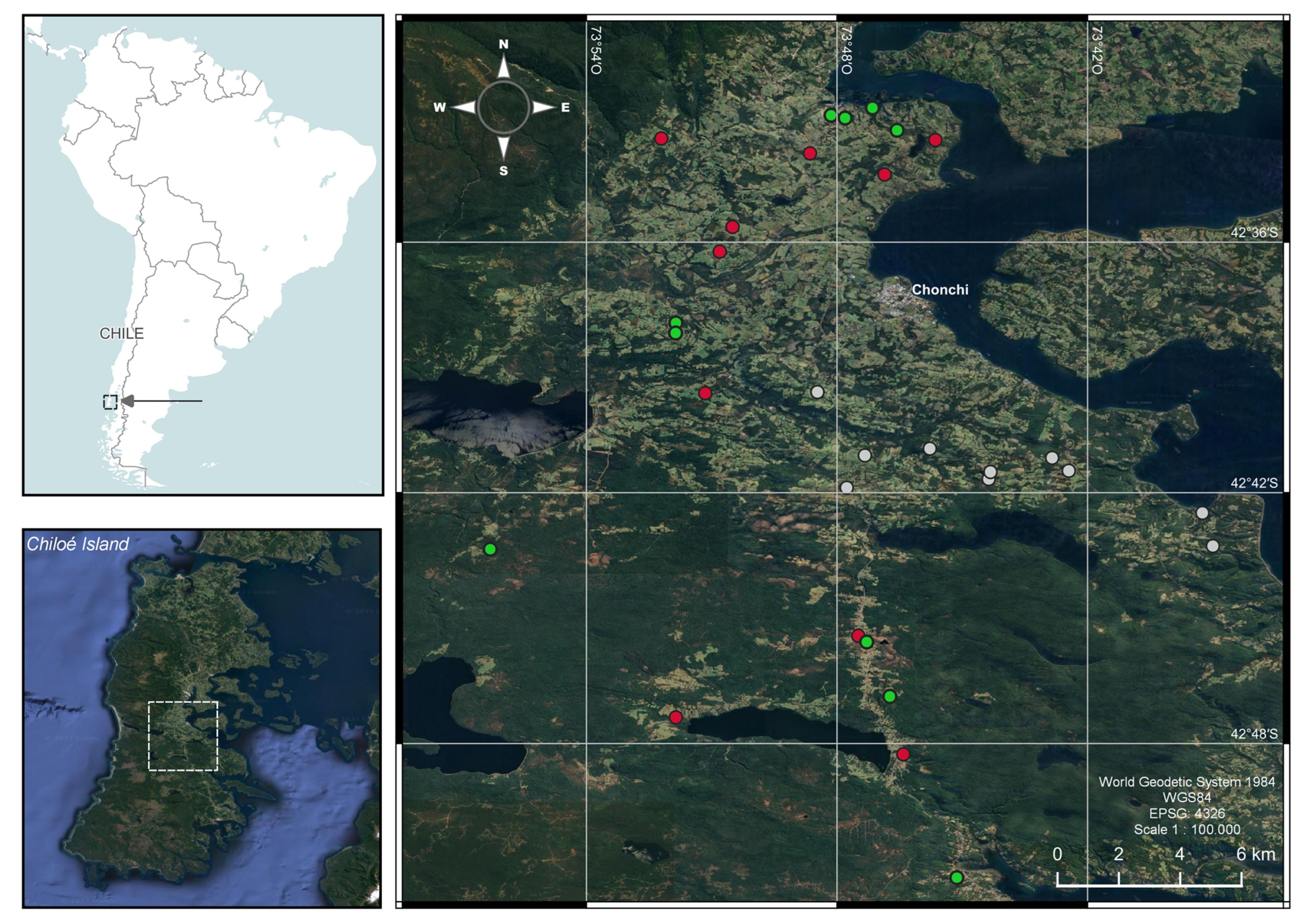
2. Materials and Methods

The study was carried out in the commune of Chonchi, located in the central zone of Chiloé Island (Figure 1; 42°40′36″ S, 73°59′36″ W), which is representative of the agricultural area of the Chiloé archipelago (Figure 1). The climate is temperate, the average annual temperature is 10.2 °C and the annual rainfall is 1460 mm [30]. The main economic activities in this area are crops, livestock and seafood exploitation [31]. Regarding land use, 32% of the area is suitable for agricultural and livestock production and 68% is suitable for forest lands [32]. Farmers produce both native and exotic varieties of potatoes and vegetables and raise mainly sheep and cattle and some pigs and poultry as well [33].

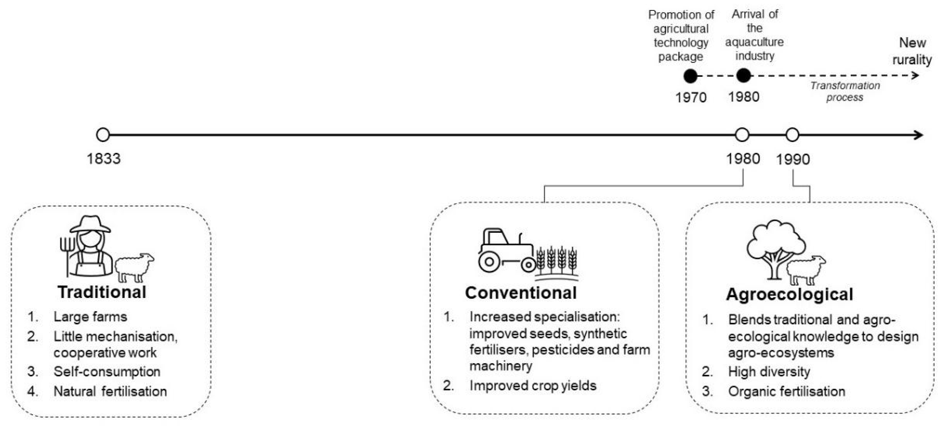
2.1. Description of Changes in Agricultural Systems and Practices

To describe the three agricultural systems (traditional, conventional and agroecological) and identify the changes that have occurred since the beginning of agriculture to the present in the study area, relevant information was collected from academic articles, agricultural census, documents prepared by Chilean government offices (Agricultural Research Institute, INIA; Office of Agricultural Studies and Policies, ODEPA; Agricultural Development Institute, INDAP; Agricultural and Livestock Service, SAG) and a non-governmental organisation (Centre for Education and Technology—Chiloé, CET) and from a field survey that will be described in the following section.

2.2. Comparison of Agricultural Systems

We developed and applied a survey (Supplementary Material Table S1) to thirty farmers (10 traditional, 10 conventional and 10 agroecological) between September and October 2021. Small farmers were selected from the database of the Local Development Program of the Chilean Ministry of Agriculture (PRODESAL), which works with 342 farmers in the Chonchi commune. The traditional system, 75% of all farmers, corresponds to a remnant of what existed in the past, characterised by crop rotation, use of animals in farming, cooperative work between peasants and production for self-consumption [24]. The conventional system, 15% of all farmers, was installed with the green revolution and the arrival of the salmon industry, and is characterised by a higher specialisation, greater technology, inclusion of pesticides and synthetic fertilisers [34]. Finally, the agroecological system, 10% of all farmers, is recognised as a sustainable agricultural and forestry system based on agroecological principles and for promoting the conservation of native potatoes [35]. According to this, our sample of 10 farmers represented 4%, 19% and 29% of each system, respectively. The survey was designed meeting the criteria required by the Cool Farm Tool (CTF) model to estimate GHG emissions [36] and the data collected represent the activities carried out every year in each farm.
For statistical analyses, we selected the 14 most representative variables from the survey and grouped them into four categories for discussion purposes (Table 1). First, we tested for differences for each of the variables between types of agriculture with a Kruskal–Wallis test and then, in cases where there were statistically significant differences, a Mann–Whitney U test of multiple comparisons. As some farmers did not perform all the activities, the ‘zeros’ were excluded in the management and fertilisation categories. In a second stage, we used multivariate approximation with a principal component analysis and later an analysis of similarities (ANOSIM) to evaluate differences among the three agricultural systems, considering the 14 variables described in Table 1. Statistical analyses were performed using PAST3 software [37].

2.3. GHG Emission Calculation for Different Agricultural Systems

Using the data collected from the surveys applied to 10 farmers of each agriculture type (Supplementary Material Table S1), the CFT (available at https://app.coolfarmtool.org/; Cool Farm Alliance, 2020, accessed on 1 November 2021) was used for estimating GHG emissions. CFT calculates GHG emissions from agricultural systems by integrating different globally determined empirical models [38,39]. Briefly, to estimate N2O emission from soil by fertiliser application, CFT uses the model by Bouwman et al. (2002) [40]. and the pesticide emission factor is derived from Audsley (1997) [41]; for land use change, tillage practices, manure management system, composting and waste management, the Intergovernmental Panel on Climate Change guidance is followed (IPCC, 2006) [42]; for livestock feed uses, the formula is derived from Hillier et al. (2011) [38]; use of fossil fuels is based on the ASAE model (2006) [43]; and for energy use it applies emission factors from a GHG protocol (2003) [44].
CFT estimates emissions of CO2, N2O, CH4 and total CO2-eq, considering the warming potential of CH4 and N2O as 25 and 298 times that of CO2, respectively [45]. The estimation was carried out at farm level for the period of one year by independently assessing crops, potatoes, cattle and other livestock. The following input data were used: (i) crops: cultivated area, yield, fertilisers and pesticides applied, irrigation and energy used for different processes, and (ii) livestock: number of animals, feed and manure management [28]. In CFT, the cattle assessment includes the grassland used and its fertilisation, while the assessment for other livestock types (in this case mainly sheep) does not consider these emissions. Therefore, when sheep grazed on land other than that of cows, general crop assessments were used to account for emissions from those grasslands. Then, the sources of emission from the CFT results had to be reorganised in order to standardise and compare between productive activities (Supplementary Material Figure S1).
Values that were unknown to the farmers were estimated based on the literature or provided by PRODESAL staff. Subsequently, the CFT assessments were completed for each farm and the results of all productive activities (Supplementary Material Figure S1) were added together to obtain the total emission for each farm and converted to kg CO2-eq ha−1 year−1.
Normality and homoscedasticity of data were tested using Shapiro–Wilk [46] and Levene tests [47]. Accordingly, mean total emissions by type of agriculture were compared using the ANOVA test [48]. For each productive activity, a Kruskal–Wallis test [49] was carried out to assess the existence of significant differences in emissions for the different types of agriculture. In addition, emissions per unit of product were obtained for each productive activity, i.e., kilograms produced for potatoes and grassland, units for vegetables and livestock units for cattle and sheep. These data were analysed using the Kruskal–Wallis test to assess the existence of significant differences. All statistical analyses were performed using R software.
As not all the farmers carried out the same productive activities or practices, to analyse how each contributed to the total emissions by agricultural type, pie charts were generated by adding the emissions of all 10 farmers. The same was carried out for the proportion of the different GHGs for each agricultural system.

3. Results

3.1. Historical Evolution of Farming Systems

Traditional agriculture has existed on the island since approximately 1833, characterised by large farms with a small productive part, little agricultural mechanisation, use of organic fertilisers and cooperative work among farmers [24,25,26]. This system remained intact until 1970 when the conventional agricultural technology package of the green revolution was installed on the island and then, in 1980, the salmon industry arrived, capturing a large part of the young peasant labour force, which is what most radically modified the Chiloé way of life [26,50,51,52]. Thus, two new types of agriculture emerged almost in parallel, first the conventional system in 1980 characterised by the use of genetically improved seeds, pesticides and machinery to work the land [24,25,53] and then in 1990 the agroecological system appeared thanks to the intervention and technology transfer of the CET (Figure 2), characterised by small and diverse farms, conserving native varieties of potatoes, in addition to the extensive use of organic fertilisers [35].
The evolution of farming systems on Chiloé Island can be summarised by four transformation processes:

3.1.1. Replacement of Organic Fertilisers and Pesticides by Chemicals

Since 1930, in Chile the use of synthetic fertilisers and agricultural machinery was encouraged to improve yields. On Chiloé, this did not take hold due to the high cost of these new products and the deep cultural roots [53]. It was thanks to state institutional policies that farmers on Chiloé incorporated these new technologies [26,33]. During field work, it was observed that conventional agriculture has incorporated the use of agrochemicals more strongly, while traditional and agroecological systems still use organic fertilisers. In addition, conventional agriculture has incorporated concentrates to feed cows and sheep in winter.

3.1.2. Disappearance of the Collaborative Work or minga and Replacement of Human Labour by Machinery

The minga is a peasant tradition of collaboration among neighbours and friends to carry out a big task, such as harvesting potatoes [54]. With the arrival of the aquaculture industry, many of the young people from the countryside have migrated to the cities [27,55], so this tradition has practically disappeared and has been replaced by paid labour, causing farmers to have had to use of machinery for sowing and harvesting to save time [26,27,28,29,30,31,32,33,34,35,36,37,38,39,40,41,42,43,44,45,46,47,48,49,50,51,52,53,54,55,56]. In 1955, there were 19 tractors in Chiloé and 361 in 2007, while in 1955 there were 75,000 people working on farms and only 29,000 in 2007 [57,58]. As observed during fieldwork, in general, the incorporation of machinery is a widespread phenomenon throughout the island, it is present in all agricultural systems, with only a few exceptions where the minga is still practised.

3.1.3. Decrease in Crop Diversity

Chiloé is one of the origin centres of the potato, its inhabitants have developed and perfected the crop and today there are more than 200 varieties [59]. However, in recent years the farmers of Chiloé have concentrated on the production of a few commercial varieties to achieve a better yield, so that today the native potato shows little genetic renewal and a loss of productive potential [60]. During fieldwork, it was observed that conventional agriculture concentrates more on commercial varieties to achieve better yields, while agroecological agriculture promotes diversity and the cultivation of native potatoes. Regarding grassland management, in conventional agriculture one or three species are sown, while agroecological agriculture promotes the diversity of forage species [33].

3.1.4. Decrease in the Total Agricultural Area

Increasingly fewer hectares of Chiloé are dedicated to agriculture, from 675,000 hectares in 1955 to 357,000 hectares in 2007 [57,58]. Potato cultivation went from 7800 ha in 1977 to 3306 ha in 2007. The same situation occurs with wheat; however, its near disappearance is due more to climatic reasons, reduction of crop rotation area and lack of labour, in addition to greater access to flour and bread already produced. Thus, wheat went from 4,371 ha in 1977 to only 180 ha in 2007 [52,58,61,62].

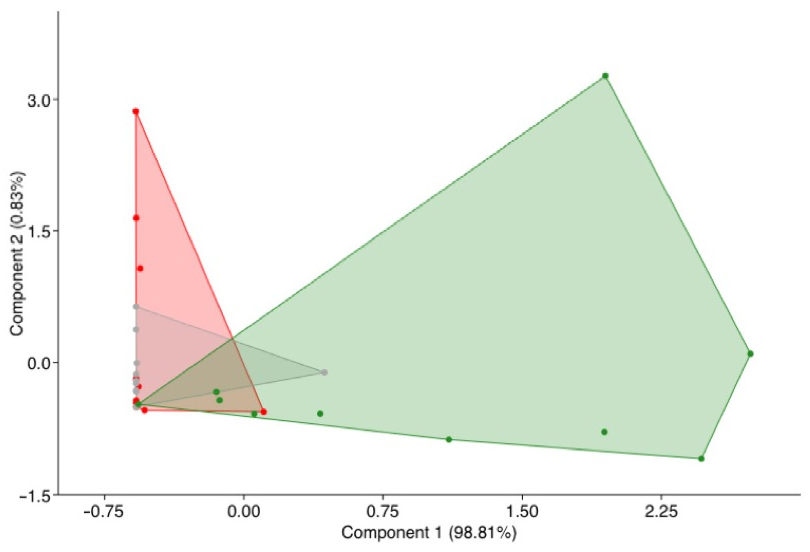
3.2. Comparison of Agricultural Systems

We found statistical differences in four out of five land use variables (except forest area) (Table 2). The traditional system has the largest area of grassland, while the conventional has the largest area of potato crop, and the agroecological system has a larger area of vegetables and the smallest total area (approximately half of the others) (Table 2). In relation to livestock variables, there were no differences between groups. For management variables, we found differences in crop richness (the lowest for conventional) and potato yield (the highest for conventional), while in the fertilisation variables only the amount of organic fertiliser used showed statistically significant differences, being higher in the agroecological system.
The principal component analysis showed an overlap between the traditional and conventional systems, while the agroecological system is separate (Figure 3). This is confirmed by the analysis of similarities (p < 0.01; R = 0.23), where no statistically significant differences are observed between the traditional and conventional systems (p > 0.05), but between these two with the agroecological system (p < 0.05; Supplementary Material Tables S2 and S3 and Figures S2 and S3). The first principal component (PC1) explains 98.8% of the variability and is strongly associated with the amount of organic and mineral fertilisers used. The second principal component explains 0.83% of the variance and is related to mineral and synthetic fertiliser (Supplementary Material Tables S4 and S5; Figures S4 and S5).

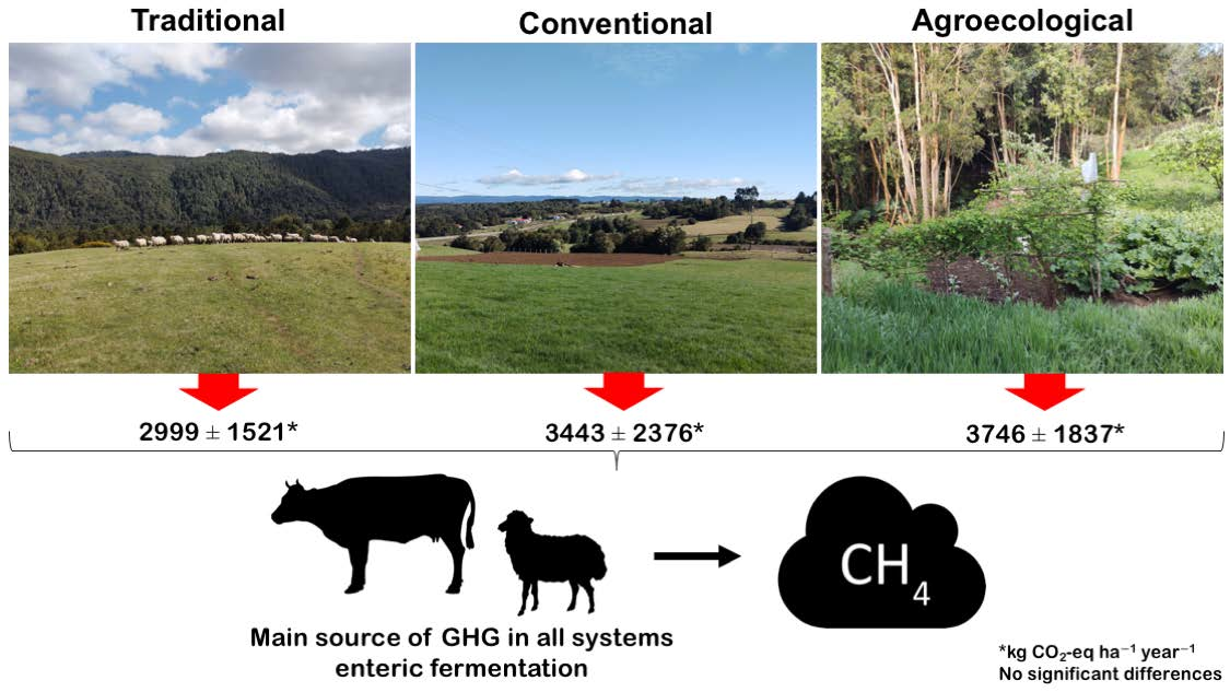
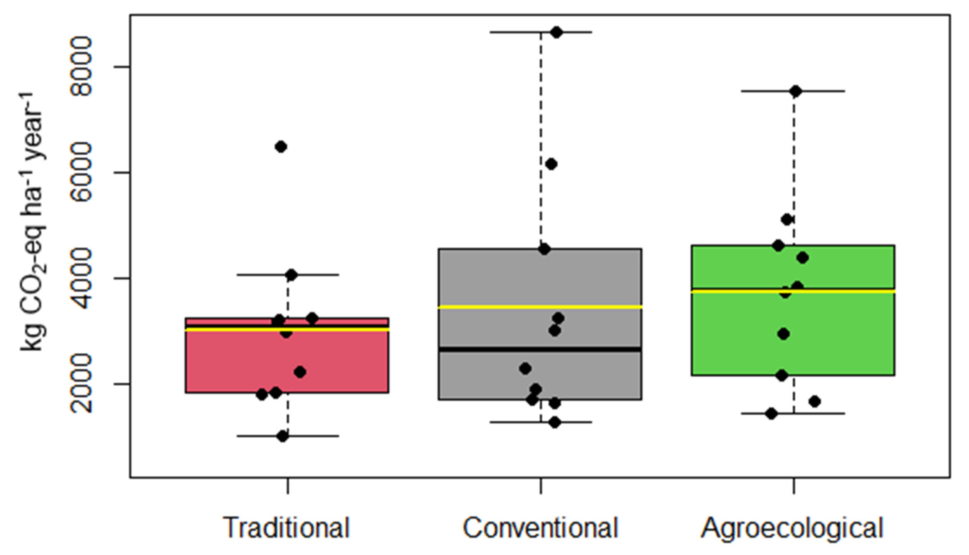
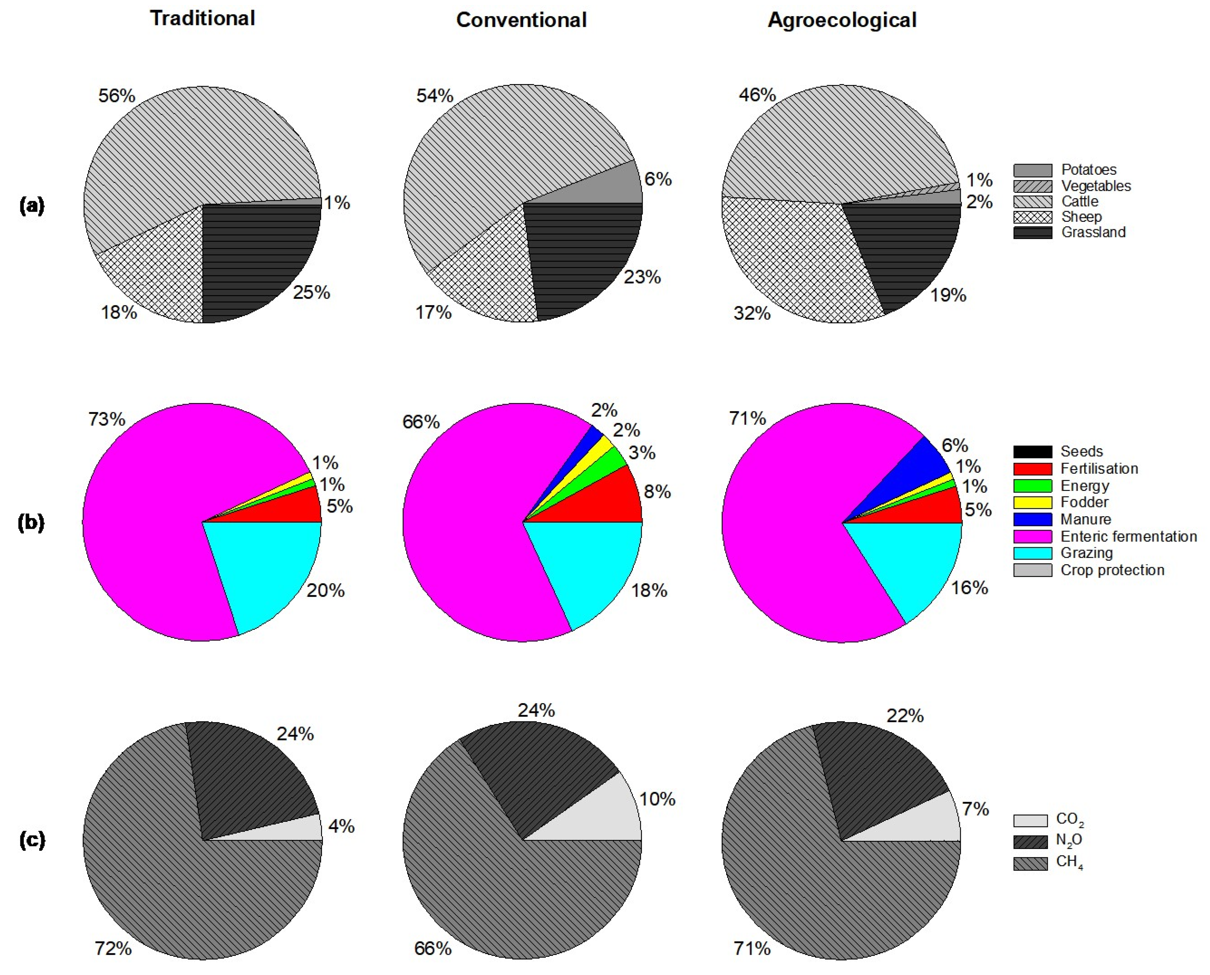
3.3. GHG Emissions of the Different Agricultural Systems

The total farm emissions per hectare in one year were on average 2999 ± 1521, 3443 ± 2376 and 3746 ± 1837 kg CO2-eq ha−1 year−1 (traditional, conventional and agroecological, respectively) and showed no significant differences among agricultural systems (p-value = 0.693), which is consistent with a wide dispersion in the emission values in the three systems, as can be seen in Figure 4. The minimum emission values were around 1000 kg CO2-eq ha−1 year−1 in all three systems, while the maximum was reached by a conventional farm at around 8500 kg CO2-eq ha−1 year−1. The summary of the medians and the significant differences obtained per productive activity for the emission analysis per hectare and per unit of product can be seen in Table 3. The highest emissions per hectare came from cattle, followed by vegetables and potatoes, while the lowest value came from grassland. Significant differences exist only in emissions per Mg of potatoes produced, conventional agriculture emits less than half as much GHG per unit of potato as other agriculture. The contributions (%) of CO2, N2O and CH4 emitted per hectare per year by crop and animal category are presented in Supplementary Material Table S6. Figure 5 shows the percentage that each productive activity contributed to the total emission. In all three systems, about half of the emissions were generated by cattle. Considering total animal emissions, i.e., cattle, sheep and grassland, the percentage is higher than 90% in all systems. Then, the crops (potatoes and vegetables) are only 6% in the case of conventional farming and less in the other two systems. When looking at the specific activities and management practices, in the three systems it was enteric fermentation that represented the highest proportion of emissions, around 70% (Figure 5b).
The contribution of CO2, CH4 and N2O to the total emissions was very similar for all three systems (Figure 5c). Methane contributes about 70% of the total, its only source was enteric fermentation, followed by N2O, with a contribution of about 20%, with sources such as fertiliser application, manure management and natural soil emissions (grazing). In the conventional system, the sources of CO2 are fossil or electric energy used for irrigation and machinery, fertiliser production and application and manure management.

4. Discussion

4.1. The Coexistence of Three Agricultural Farming Systems

According to the bibliographical sources [18,19,20,21,22,23,24,25,26,27,28,29,30,31,32,33,34,35,36,37,38,39,40,41] and the local state agency that advises farmers (PRODESAL), three different agricultural systems currently coexist on Chiloé. However, according to our multivariate analyses, the conventional system does not differ from the traditional one (Figure 3). This is possibly the result of the restructuring of the rural sector in Chile as a part of the neoliberal policies and the implementation of industrial agriculture in the 1970s [63] that arrived approximately a decade later on Chiloé due to its isolated geography (Figure 2) [26,52]. This means that the new technology was partly assimilated by the pre-existing traditional farmers, mainly by substituting animal traction by machinery and by replacing organic fertilisers for synthetic ones, while some traditional practices are still preserved. However, when we carried out the analysis comparing each of the variables, we observed that those associated with potato production (crop area and yield) were the ones in which these two systems differed, which suggests that the conventional system would be characterised by greater specialisation in potato production (Table 2).
In the same way, the properties that would currently be considered conventional are possibly derived directly from the traditional system that tended towards the intensification and specialisation of their management practices. For example, many of these farms have concentrated on growing certified potato varieties to improve their yields, leaving aside the cultivation of native potatoes [33], therefore, nowadays it is difficult to separate these two farming systems. Regarding the degree of specialisation of the conventional system, a significant decrease in the number of crops was observed (Table 1). This coincides with experiences in other parts of the world, such as the European Alps, where the transition towards modern practices results in deterioration of local biodiversity, suggesting that state subsidies are necessary to maintain practices that are more compatible with biodiversity [64].
On the other hand, the agroecological system is significantly different from the traditional and conventional systems, showing among other differences a smaller total cultivated area and a higher proportion of this area dedicated to growing vegetables (Table 2). The agroecological farms of Chiloé belong to the Globally Important Agricultural Heritage Systems (GIAHSs) because they integrate Huilliche ancestral knowledge with elements of modern science and have been fundamental in the recovery and conservation of the germplasm of the native potato [35,65]. This type of complex and multispecies agricultural system tends to be more resilient to environmental variations, so in addition to conserving an agricultural heritage, it contributes to the conservation of biodiversity [35].

4.2. Greenhouse Gas Balance of Different Types of Agriculture

The mean GHG emissions from the three agricultural systems (3396 kg CO2-eq ha−1 year−1) can be compared with a previous study that estimated the GHG balance in this region on croplands (9010 kg CO2-eq ha−1 year−1) and grasslands (−13,500 kg CO2-eq ha−1 year−1), although these estimations were based on direct measurements and did not differentiate between agricultural systems [66]. Our estimations are smaller than those reported for European farms, for both organic and conventional systems (5450 ± 2720 and 11,342 ± 3443 kg CO2-eq ha−1 year−1, respectively) [6]. In this study, we found that although there are differences in the agricultural practices among the farming systems, particularly between the agroecological systems compared to the traditional and conventional systems, there are no significant differences in GHG emissions between them (Figure 4). Similar results were obtained by Dendooven et al. [67], who analysed the differences in GHG emissions in two tillage systems (1: a no-tillage system with crop rotation and residue retention in the soil; 2: a conventional tillage system with residue removal and maize monoculture), and found that they had little impact on emissions, but did have significant effects on soil carbon storage. In addition, Astier et al. [68] studied the differences in GHG emissions between conventional and organic avocado cultivation and found no significant differences.
Flessa et al. [69] evaluated GHG emissions from two farming systems in southern Germany and found that the largest contribution to GHG emissions in agricultural systems was from N2O, about 60%, 25% from methane and 15% from CO2. The authors related the high contribution of N2O to the application and production of fertilisers, which are mainly used in crops that cover about 70% of the total area. In our study, crops cover only around 10% of the farm, which likely explains why N2O contributed only about 23% of the emissions. Meanwhile, high agreement was found between our results for the conventional system and those from a study that looked at cattle pastoral farms in the Netherlands (no crops), with a stocking rate of 2.2 animal units ha−1, where the emissions were 64% from CH4, 26% from N2O and 9% from CO2 [70].
Worldwide, ruminant livestock production contributes significantly to GHG emissions, mainly through the enteric fermentation process that releases methane (CH4) [71], which is the main GHG contributing to climate change after CO2 [72]. In this study, enteric fermentation (from cattle and sheep) was the largest source of emissions in all three agricultural systems (traditional, conventional and agroecological). In this sense, it is especially important to apply management practices that mitigate this type of emission [73], which are mainly related to managing the stocking rate and feeding supplementation. In the first case, it is suggested to maintain relatively low stocking rates [74,75]. In this study, even though the conventional system showed a higher stocking rate of cattle, the difference was not significant, which explains why there were no significant differences in emissions related to cattle raising (Table 3). This is possibly because although the traditional and conventional systems incorporate more practices from industrial agriculture than the agroecological system, they still use relatively low cattle stocking rates (1–2 animal units ha−1; Table 2) compared, for example, to the livestock-intensive systems in Brazil (3–4 animal units ha−1) [76]. A low stocking rate has been highlighted as one of the most important management decisions related to GHG emissions, animal welfare and the conservation of biodiversity in grazing sites [77,78]. In this sense, it would be interesting to investigate the mechanisms associated with the stocking rate and GHG emissions in the agricultural systems of Chiloé. Within the conceptual framework of FAO-GIAHS, multifunctional systems such as the Barroso Agro-Silvo-Pastoral System in Portugal are considered more resilient to the challenges of global change [79]. Regarding feeding supplementation, it was observed that the incorporation of plants with bioactive compounds (10% leaves of lemon grass (Cymbopogon citratus) and curry (Murraya koenigii)) to the diet of lambs resulted in a decrease in CH4 emissions [80]. In the same way, the use of red algae (Asparagopsis taxiformis) in the diet of cattle reduced the CH4 production [81]. Considering that these kinds of supplements are usually imported, their use could have an undesirable effect on CO2 emissions from transport [13]. For this reason, it would be interesting to investigate how plants or algae locally available on Chiloé can contribute to the reduction of GHG emissions.
Nitrous oxide was the second most abundant gas in the three systems, originated mainly by fertilisation practices. Therefore, the stabilisation of organic matter (compost and manure) is recommended before its application [82,83], for example, through the incorporation of inorganic materials such as fly ashes during the composting process [84]. There is also evidence that the use of biochar during composting is a way to mitigate the GHG emissions that are released during this process [85]. In the case of mineral nitrogen, the recommendation is to apply it in dry weather periods [86], which could be a difficulty in environments with high rainfall such as southern Chile.

4.3. Limitations of the Study and Future Research

The Chonchi commune was found to be representative of the farming systems on the Chiloé archipelago. However, it is important to point out that farmers in this area do not keep accurate records of their management practices, so the input data for estimating GHG emissions were an approximation in some cases. In this sense, rather than increasing the number of farms, we think it would be more informative to study in more detail some of the farms that are more representative of each farming system.
Among the available tools for estimating GHG emissions at the farm level, the Cool Farm Tool (CFT) has been used in different types of climates and farming conditions [87,88,89,90]. One advantage of CFT is that it requires input data generally known to the farmer, making it useful for decision support at the farm scale and also to inform practices and their impact [38]. However, one of the limitations of the CFT model is that it does not consider leaving manure on the field as a management practice. The CFT methodological guide mentions pasture/grazing manure management, but later in the tool there is no such option; therefore, when a farmer left manure on the field, no manure management was assigned. On the other hand, CFT does include composting manure management, which is mainly used by agroecological and traditional agriculture, and in this case manure management was included. This could have led to an underestimation in farms that kept large numbers of livestock and left the manure in the field, particularly in the emissions of N2O, since this gas is produced mainly from the manure [91]. Additionally, the bovine assessment includes the grazing livestock pasture, while for the other livestock species it does not, so a separate crop assessment had to be generated to account for the sheep pasture emissions, which made it difficult to compare the main management activities. This is because CFT is a calculator focused on measuring emissions by product [45]. Finally, because CFT does not account for GHG capture, in this study we only estimated the GHG emissions of each agricultural system. In the future, using other tools that also include carbon removals, such as IPCC guidelines [42], may show differences in the GHG balance, particularly because the systems show differences in the amount of organic fertiliser used and the area covered by forests.
The results obtained in this research raise questions that may require more information to be collected or even experimental approaches to be used. A relevant question is whether agricultural systems differ in their ability to store carbon and capture GHG, which would complement what was observed through modelling [92]. In this sense, analysing soil microbial diversity and activity could provide information about the mechanisms behind the observed patterns and in the future incorporate this dimension into sustainable management practices [93]. Understanding the dynamics of the soil microbiota and its management (such as the incorporation of agricultural stubble) can contribute to the mitigation of GHG emissions, since microorganisms play a fundamental role in the stabilisation of carbon and nitrogen in soil [94].
Like many other countries that export goods derived from agriculture and livestock, Chile faces great challenges associated with climate change, being ranked as the country with the 18th highest water shortage due to climate change and growing demand [95]. Accordingly, it is in the process of reducing its GHG emissions, has signed the Paris Agreement [96] and committed to becoming carbon-neutral by 2050 [97]. Although Chile contributed only 0.23% to global emissions in 2020 [98], its emissions have recently increased significantly, with agriculture being the second largest contributor (10.5% in 2018) after power generation [99]. Our work is in line with detecting which practices generate the most emissions in different agricultural systems, in order to focus attention on how to improve their management.

5. Conclusions

Traditional farming has been practised on Chiloé since ~1830 and is one of the Globally Important Agricultural Heritage Systems. After the incorporation of modern techniques in the 1980s, several farms were classified as conventional; however, according to our analyses, these two types are not significantly different. Subsequently, in the 1990s, a group of farmers combined ancestral and modern ecological knowledge, forming the agroecological farming system, which in fact does differ from the other two systems. The traditional–conventional systems are relatively large farms, specialised in the production of cattle or potatoes, whereas the agroecological farms are significantly smaller and are mainly used to grow vegetables.
Even though we found differences in land use and management practices between agricultural systems in southern Chile, these differences were not observed in the total GHG emissions. The emissions of the three systems are relatively low compared to other livestock systems such as European dairy farms. All three systems showed a higher proportion of emissions related to animal production, mainly explained by enteric fermentation of livestock. In turn, crop emissions were very low, which matches with the low proportion of cultivated area. Therefore, to reduce GHG emissions in all three types of agriculture in this area, it would be necessary first to incorporate management practices focused on reducing the CH4 emissions from livestock, and secondly to reduce N2O emissions from fertilisers.

Supplementary Materials

The following supporting information can be downloaded at: https://www.mdpi.com/article/10.3390/agronomy13010240/s1, Table S1: Field survey; Table S2: ANOSIM (similarity index: Euclidean); Table S3: Pairwise comparisons with Bonferroni correction; Table S4: Summary PCA (variance–covariance matrix); Table S5: PCA loadings; Table S6: Contribution (%) of CO2, N2O and CH4 per hectare and year by crop and animal category; Figure S1: CFT emission source reorganisation; Figure S2: Analyses of similarities (ANOSIM); Figure S3: Agricultural system hierarchical clustering; Figure S4: PC1 correlation plot; Figure S5: PC2 correlation plot.

Author Contributions

Conceptualisation, F.M., J.F.P.-Q. and N.M.; methodology, F.M., J.F.P.-Q. and N.M.; software, F.M.; formal analysis, F.M. and C.S.; writing—review and editing, F.M, C.S., J.F.P.-Q. and N.M.; supervision and funding acquisition, J.F.P.-Q. All authors have read and agreed to the published version of the manuscript.

Funding

Funding was provided by the New Zealand Government to support the objectives of the Global Research Alliance on Agricultural Greenhouse Gases. The authors also acknowledge the support of the University of Chile through its Program for Institutional Excellence (PEEI), and the National Agency for Research and Development (ANID-Chile) through grants PIA/BASAL FB210006 (Institute of Ecology and Biodiversity) and FB210018 (Cape Horn International Center). This work is part of the ReLive project, funded by the Joint Call of the Cofund ERA-Nets SusCrop (Grant N° 771134), FACCE ERA-GAS (Grant N° 696356), ICT-AGRI-FOOD (Grant N° 862665) and SusAn (Grant N° 696231).

Informed Consent Statement

Informed consent was obtained from all subjects involved in the study.

Data Availability Statement

Data will be provided upon request.

Acknowledgments

The authors thank Bárbara Gómez and all the staff of PRODESAL at Chonchi (Ministry of Agriculture) for the technical support to contact the farmers and their help during the field campaign, Pia Gottschalk for her help with the CFT software and Vicente Arriagada for his help with map preparation. This work was possible thanks to the kind cooperation of the thirty farmers who provided the information used in our study.

Conflicts of Interest

The authors declare no conflict of interest. The funders had no role in the design of the study nor in the decision to publish the results.

References

  1. Allen, M.; Babiker, M.; Chen, Y.; de Coninck, H. IPCC SR15: Summary for policymakers. In IPCC Special Report Global Warming of 1.5 °C; Intergovernmental Panel on Climate Change: Geneva, Switzerland, 2018; Available online: https://research.tue.nl/en/publications/ipcc-sr15-summary-for-policymakers (accessed on 19 November 2022).
  2. Shukla, P.R.; Skeg, J.; Buendia, E.; Masson-Delmotte, V.; Pörtner, H.-O.; Roberts, D.C.; Zhai, P.; Slade, R.; Connors, S.; van Diemen, S.; et al. Special Report on Climate Change, Desertification, Land Degradation, Sustainable Land Management, Food Security, and Greenhouse Gas Fluxes in Terrestrial Ecosystems. 2019. Available online: https://philpapers.org/rec/SHUCCA-2 (accessed on 19 November 2022).
  3. Alexandratos, N.; Bruinsma, J. World Agriculture: Towards 2015/2030: An FAO Study; Routledge: London, UK, 2017; pp. 1–431. [Google Scholar] [CrossRef]
  4. Kohler, F.; Thierry, C.; Marchand, G. Multifunctional agriculture and farmers’ attitudes: Two case studies in rural France. Hum. Ecol. 2014, 42, 929–949. [Google Scholar] [CrossRef]
  5. Garnier, J.; Le Noë, J.; Marescaux, A.; Sanz-Cobena, A.; Lassaletta, L.; Silvestre, M.; Thieu, V.; Billien, G. Long-term changes in greenhouse gas emissions from French agriculture and livestock (1852–2014): From traditional agriculture to conventional intensive systems. Sci. Total Environ. 2019, 660, 1486–1501. [Google Scholar] [CrossRef]
  6. Olesen, J.E.; Schelde, K.; Weiske, A.; Weisbjerg, M.R.; Asman, W.A.H.; Djurhuus, J. Modelling greenhouse gas emissions from European conventional and organic dairy farms. Agric. Ecosyst. Environ. 2006, 112, 207–220. [Google Scholar] [CrossRef]
  7. Lee, K.S.; Choe, Y.C.; Park, S.H. Measuring the environmental effects of organic farming: A meta-analysis of structural variables in empirical research. J. Environ. Manag. 2015, 162, 263–274. [Google Scholar] [CrossRef] [PubMed] [Green Version]
  8. Tuomisto, H.L.; Tuomisto, H.L.; Riordan, P.; Macdonald, D.W. Does organic farming reduce environmental impacts? A meta-analysis of European research. J. Environ. Manag. 2012, 112, 309–320. [Google Scholar] [CrossRef]
  9. Gaitán, L.; Läderach, P.; Graefe, S.; Rao, I.; van der Hoek, R. Climate-smart livestock systems: An assessment of carbon stocks and GHG emissions in Nicaragua. PLoS ONE 2016, 11, 0167949. [Google Scholar] [CrossRef] [PubMed] [Green Version]
  10. Morgan, J.A.; Follett, R.F.; Allen, L.H.; Del Grosso, S.; Derner, J.D.; Dijkstra, F.; Franzluebbers, A.; Fry, R.; Paustian, K.; Schoeneberger, M.M. Carbon sequestration in agricultural lands of the United States. J. Soil Water Conserv. 2010, 65, 6A–13A. [Google Scholar] [CrossRef] [Green Version]
  11. West, T.O.; Post, W.M. Soil organic carbon sequestration rates by tillage and crop rotation: A global data analysis. Soil Sci. Soc. Am. J. 2002, 66, 1930–1946. [Google Scholar] [CrossRef] [Green Version]
  12. Ford, H.; Healey, J.; Webb, B.; Pagella, T.F.; Smith, A.R. How do hedgerows influence soil organic carbon stock in livestock-grazed pasture? Soil Use Manag. 2019, 35, 576–584. [Google Scholar] [CrossRef]
  13. Sintori, A.; Liontakis, A.; Tzouramani, I. Assessing the environmental efficiency of greek dairy sheep farms: GHG emissions and mitigation potential. Agriculture 2019, 9, 9020028. [Google Scholar] [CrossRef] [Green Version]
  14. Roque, B.M.; Salwen, J.K.; Kinley, R.; Kebreab, E. Inclusion of Asparagopsis armata in lactating dairy cows’ diet reduces enteric methane emission by over 50 percent. J. Clean. Prod. 2019, 234, 132–138. [Google Scholar] [CrossRef]
  15. Wassmann, R.; Papen, H.; Rennenberg, H. Methane emission from rice paddies and possible mitigation strategies. Chemosphere 1993, 26, 201–217. [Google Scholar] [CrossRef]
  16. Lamb, W.F.; Wiedmann, T.; Pongratz, J.; Andrew, R.; Crippa, M.; Olivier, J.G.J.; Wiedenhofer, D.; Mattioli, G.; Al Khourdajie, A.; House, J.; et al. A review of trends and drivers of greenhouse gas emissions by sector from 1990 to 2018. Environ. Res. Lett. 2021, 16, 073005. [Google Scholar] [CrossRef]
  17. Smith, P.; Martino, D.; Cai, Z.; Gwary, D.; Janzen, H.; Kumar, P.; McCarl, B.; Ogle, S.; O’Mara, F.; Rice, C.; et al. Greenhouse gas mitigation in agriculture. Philos. Trans. R. Soc. B Biol. Sci. 2008, 363, 789–813. [Google Scholar] [CrossRef] [PubMed] [Green Version]
  18. He, Z.; Zhang, Y.; Liu, X.; de Vries, W.; Ros, G.H.; Oenema, O.; Xu, W.; Hou, Y.; Wang, H.; Zhang, F. Mitigation of nitrogen losses and greenhouse gas emissions in a more circular cropping-poultry production system. Resour. Conserv. Recycl. 2023, 189, 106739. [Google Scholar] [CrossRef]
  19. Heeb, L.; Jenner, E.; Cock, M.J.W. Climate-smart pest management: Building resilience of farms and landscapes to changing pest threats. J. Pest. Sci. 2019, 92, 951–969. [Google Scholar] [CrossRef]
  20. Schut, A.G.T.; Cooledge, E.; Moraine, M.; van de Ven, G.W.J.; Jones, D.L.; Chadwick, D. Reintegration of crop-livestock systems in Europe: An overview. Front. Agric. Sci. Eng. 2021, 8, 111–129. [Google Scholar] [CrossRef]
  21. Regan, J.T.; Marton, S.; Barrantes, O.; Ruane, E.; Hanegraaf, M.; Berland, J.; Korevaar, H.; Pellerin, S.; Nesme, T. Does the recoupling of dairy and crop production via cooperation between farms generate environmental benefits? A case-study approach in Europe. Eur. J. Agron. 2017, 82, 342–356. [Google Scholar] [CrossRef] [Green Version]
  22. Economic Commission for Latin America and the Caribbean. Prospects for Agriculture and Rural Development in the Americas: A Look at Latin America and the Caribbean. 2012. Available online: https://repositorio.cepal.org/handle/11362/1462 (accessed on 21 November 2022). (In Spanish).
  23. Food and Agriculture Organization of the United Nations. Important World Agricultural Heritage Systems, Agriculture Chiloé, Chile; Agricultura Chiloé: Chiloé, Chile, 2022; Available online: https://www.fao.org/giahs/giahsaroundtheworld/designated-sites/latin-america-and-the-caribbean/chiloe-agriculture/partners/en/ (accessed on 21 November 2022). (In Spanish)
  24. Saliéres, M.; Le Grix, M.; Vera, W.; Billaz, R. La agricultura familiar chilota en perspectiva. Rev. Lider 2005, 13, 79–104. [Google Scholar]
  25. Barrena, J.; Nahuelhual, L.; Báez, A.; Schiappacasse, I.; Cerda, C. Valuing cultural ecosystem services: Agricultural heritage in Chiloé island, southern Chile. Ecosyst. Serv. 2014, 7, 66–75. [Google Scholar] [CrossRef]
  26. Bravo, J.M.; Zúñiga, R.; Oyanedel, N.F. Chiloé Smallholdings: The Evolution of an Ancestral Agricultural Tenure in a Globalizing Context (Isla Quinchao, Chile). Quántica 2021, 2, 32–41. Available online: https://revistacuantica.com/index.php/rcq/article/download/7/66) (accessed on 5 December 2022). (In Spanish).
  27. Chiloé Education and Technology Center. Chiloé Agro-Biodiversity Cultural System Chile Project Framework | FAO. 2007. Available online: https://www.fao.org/agroecology/database/detail/en/c/442997/ (accessed on 19 November 2022).
  28. Montalba, R.; Infante, A.; Contreras, A.; Vieli, L. Agroecology in Chile: Precursors, pioneers, and their legacy. Agroecol. Sustain. Food Syst. 2017, 41, 416–428. [Google Scholar] [CrossRef]
  29. Venegas, C.; Gómez, B.; Infante, A. Agroecological Transition Manual for Peasant Family Agriculture. 2018. Available online: https://bibliotecadigital.ciren.cl/handle/20.500.13082/32260 (accessed on 1 December 2021). (In Spanish).
  30. INIA. Agrometeorological Network. Tara Station in Chonchi Commune. 2022. Available online: https://agrometeorologia.cl/TS00# (accessed on 21 November 2022). (In Spanish).
  31. Food and Agriculture Organization of the United Nations. Views, Experiences and Best Practices as an Example of Possible Options for the National Implementation of Article 9 of the International Treaty; Food and Agriculture Organization of the United Nations: Rome, Italy, 2021; Available online: https://www.fao.org/3/ca7907en/ca7907en.pdf (accessed on 19 November 2022).
  32. Gayán, A.; Dumont, J. Butalcura Experimental Center, a Chiloé Wish Come True. 1997. Available online: https://biblioteca.inia.cl/handle/20.500.14001/35707?show=full (accessed on 1 December 2021). (In Spanish).
  33. Chiloé Education and Technology Center. Chiloé Baseline Update, Project GCP/GLO/212/GFF: Conservation and Adaptive Management of Important World Agricultural Heritage Systems (GIAHS). Available online: https://www.ced.cl/cedcl/wp-content/uploads/2011/10/sipam-chiloe.pdf (accessed on 1 December 2021).
  34. Bustos, B.; Delano, J.; Prieto, M. “Salmon Type Chilote”. Relations between the Commodification of Nature and Identity Production Processes. Estudios Atacamenos. 2019, 63, 383–402. Available online: https://revistas.ucn.cl/index.php/estudios-atacamenos/article/view/1359 (accessed on 5 December 2022). (In Spanish).
  35. Altieri, M. An Agroecological Strategy in Chile as a Basis for Food Sovereignty. Ambient. Desarro. CIPMA 2010, 24, 25–29. Available online: http://agroeco.org/wp-content/uploads/2016/01/CIPMA-Altieri.pdf (accessed on 5 December 2022). (In Spanish).
  36. Cool Farm Alliance. Cool Farm Alliance. Use the Cool Farm Tool. Available online: https://coolfarmtool.org/ (accessed on 1 November 2021).
  37. Hammer, Ø.; Harper, D.A.; Ryan, P.D. Past: Paleontological Statistics Software Package for Education and Data Analysis. Palaeontol. Electron. 2001, 4, 178. Available online: http://palaeo-electronica.org/2001_1/past/issue1_01.htm (accessed on 5 December 2022).
  38. Hillier, J.; Walter, C.; Malin, D.; Garcia-Suarez, T.; Mila-i-Canals, L.; Smith, P. A farm-focused calculator for emissions from crop and livestock production. Environ. Model. Softw. 2011, 26, 1070–1078. [Google Scholar] [CrossRef]
  39. Haverkort, A.J.; Hillier, J.G. Cool Farm Tool—Potato: Model Description and Performance of Four Production Systems. Potato Res. 2011, 54, 355–369. [Google Scholar] [CrossRef] [Green Version]
  40. Bouwman, A.F.; Boumans, L.J.M.; Batjes, N.H. Modelling global annual N2O and NO emissions from fertilized fields. Glob. Biogeochem. Cycles 2002, 16, 1080 28-1. [Google Scholar] [CrossRef]
  41. Audsley, E.; Alber, S.; Clift, R.; Cowell, S.; Crettaz, P.; Gaillard, G.; Hausheer, J.; Jolliet, O.; Kleijn, R.; Mortensen, B.; et al. Harmonisation of Environmental Life Cycle Assessment for Agriculture. 1997. Available online: https://cordis.europa.eu/project/id/AIR32028 (accessed on 6 November 2021).
  42. Eggleston, L.; Buendia, K.; Miwa, T.; Tanabe, K. 2006 IPCC Guidelines for National Greenhouse Gas Inventories. 2006. Available online: https://www.ipcc-nggip.iges.or.jp/meeting/pdfiles/Washington_Report.pdf (accessed on 19 November 2022).
  43. American Society of Agricultural and Biological Engineers. ASAE EP496.3: 2013(R2011) Agricultural Machinery Management. 2013. Available online: https://infostore.saiglobal.com/en-us/standards/asae-ep496-3-2006-r2011--133265_saig_asae_asae_284765/ (accessed on 5 December 2022).
  44. Greenhouse Gas Protocol. Calculation Tools|Greenhouse Gas Protocol. 2003. Available online: https://ghgprotocol.org/calculation-tools (accessed on 19 November 2022).
  45. Cool Farm Alliance. Cool Farm Tool Technical Documentation Version 1.0 Corresponding CFT v0.11.1; Cool Farm Alliance: Grantham, UK; p. 2020.
  46. Shapiro, S.S.; Wilk, M.B. An Analysis of Variance Test for the Exponential Distribution (Complete Samples). Technometrics 1972, 14, 355–370. [Google Scholar] [CrossRef]
  47. Fox, J. Applied Regression Analysis and Generalized Linear Models; Sage Publications: Thousand Oaks, CA, USA, 2015. [Google Scholar]
  48. Chambers, J.M.; Freeny, A.E.; Heiberger, R.M. Analysis of variance; designed experiments. In Statistical Models; Chambers, J.M., Hastie, T.J., Eds.; Wadsworth & Brooks/Cole: Pacific Grove, CA, USA, 1992; Volume 5. [Google Scholar]
  49. Kruskal, W.H.; Wallis, W.A. Use of Ranks in One-Criterion Variance Analysis. JASA 1952, 47, 583–621. [Google Scholar] [CrossRef]
  50. Nahuelhual, L.; Carmona, A.; Laterra, P.; Barrena, J.; Aguayo, M. A mapping approach to assess intangible cultural ecosystem services: The case of agriculture heritage in Southern Chile. Ecol. Indic. 2014, 40, 90–101. [Google Scholar] [CrossRef]
  51. Gómez, J.E.; Amtmann, R. Chile: Expansion of Salmon Farming and Industry and Peasant Family Agriculture (New Rurality and Peasant Persistence). Rev. Sociol. 2003, 0, 149–163. Available online: https://revistadesociologia.uchile.cl/index.php/RDS/article/view/27795 (accessed on 5 December 2022). (In Spanish).
  52. Díaz, G.I.; Nahuelhual, L.; Echeverría, C.; Marín, S. Drivers of land abandonment in Southern Chile and implications for landscape planning. Landsc. Urban Plan 2011, 99, 207–217. [Google Scholar] [CrossRef]
  53. Daughters, A. Food and Culture. In Chiloé: Potatoes, Curanto, and Chicha; Springer: Cham, Switzerland, 2018; pp. 53–65. [Google Scholar] [CrossRef]
  54. Fløysand, A.; Barton, J.R.; Román, Á. The double hierarchy of economic development and local government in Chile: The case of salmon farming and Chilote municipalities. EURE 2010, 36, 123–148. (In Spanish) [Google Scholar] [CrossRef]
  55. Barton, J.R.; Fløysand, A. The political ecology of Chilean salmon aquaculture, 1982-2010: A trajectory from economic development to global sustainability. Glob. Environ. Chang. 2010, 20, 739–752. [Google Scholar] [CrossRef]
  56. Berdegué, J.A.; Bebbington, A.; Escobal, J. Conceptualizing Spatial Diversity in Latin American Rural Development: Structures, Institutions, and Coalitions. World Dev. 2015, 73, 1–10. [Google Scholar] [CrossRef]
  57. Statistics and Census Directorate. In National Agricultural Livestock Census; Government of Chile: Santiago, Chile, 1955.
  58. National Statistics Institute. VII National Agricultural and Forestry Census; Government of Chile: Santiago, Chile, 2007. (In Spanish)
  59. Esnault, F.; Solano, J.; Perretant, M.R.; Hervé, M.; Label, A.; Pellé, R.; Dantec, J.P.; Boutet, G.; Brabant, P.; Chauvin, J.E. Genetic diversity analysis of a potato (Solanum tuberosum L.) collection including Chiloé Island landraces and a large panel of worldwide cultivars. Plant Genet. Resour. 2014, 12, 74–82. [Google Scholar] [CrossRef]
  60. Spanoghe, M.; Marique, T.; Nirsha, A.; Esnault, F.; Lanterbecq, D. Genetic Diversity Trends in the Cultivated Potato: A Spatiotemporal Overview. Biology 2022, 11, 604. [Google Scholar] [CrossRef]
  61. National Statistics Institute. V National Agricultural Census; Government of Chile: Santiago, Chile, 1977. (In Spanish)
  62. National Statistics Institute. VI National Agricultural and Forestry Census; Government of Chile: Santiago, Chile, 1997. (In Spanish)
  63. Kay, C. Chile’s neoliberal agrarian transformation and the peasantry. J. Agrar. Chang. 2002, 2, 464–501. [Google Scholar] [CrossRef]
  64. Marini, L.; Klimek, S.; Battisti, A. Mitigating the impacts of the decline of traditional farming on mountain landscapes and biodiversity: A case study in the European Alps. Environ. Sci. Policy 2011, 14, 258–267. [Google Scholar] [CrossRef]
  65. Altieri, M.A.; Nicholls, C.I. Scaling up agroecological approaches for food sovereignty in Latin America. Development 2008, 51, 472–480. [Google Scholar] [CrossRef]
  66. Perez-Quezada, J.F.; Cano, S.; Ibaceta, P.; Aguilera-Riquelme, D.; Salazar, O.; Fuentes, J.P.; Osborne, B. How do land cover changes affect carbon-nitrogen-phosphorus stocks and the greenhouse gas budget of ecosystems in southern Chile? Agric. Ecosyst. Environ. 2022, 340, 108153. [Google Scholar] [CrossRef]
  67. Dendooven, L.; Gutiérrez-Oliva, V.F.; Patiño-Zúñiga, L.; Ramírez-Villanueva, D.A.; Verhulst, N.; Luna-Guido, M.; Marsch, R.; Montes-Molina, J.; Gutiérrez-Miceli, M.A.; Vásquez-Murrieta, S.; et al. Greenhouse gas emissions under conservation agriculture compared to traditional cultivation of maize in the central highlands of Mexico. Sci. Total Environ. 2012, 431, 237–244. [Google Scholar] [CrossRef] [PubMed]
  68. Astier, M.; Merlín-Uribe, Y.; Villamil-Echeverri, L.; Garciarreal, A.; Gavito, M.E.; Masera, O.R. Energy balance and greenhouse gas emissions in organic and conventional avocado orchards in Mexico. Ecol. Indic. 2014, 43, 281–287. [Google Scholar] [CrossRef]
  69. Flessa, H.; Ruser, R.; Dörsch, P.; Kamp, T.; Jimenez, M.; Munch, J.; Beese, F. Integrated evaluation of greenhouse gas emissions (CO2, CH4, N2O) from two farming systems in southern Germany. Agric. Ecosyst. Environ. 2002, 91, 175–189. [Google Scholar] [CrossRef]
  70. McDowell, R.W. Environmental Impacts of Pasture-Based Farming; Cabi: Wallingford, UK, 2008. [Google Scholar]
  71. Zhang, L.; Tian, H.; Shi, H.; Pan, S.; Chang, J.; Dangal, S.R.S.; Qin, X.; Wang, S.; Tubiello, F.N.; Canadell, J.G.; et al. A 130-year global inventory of methane emissions from livestock: Trends, patterns, and drivers. Glob. Chang. Biol. 2021, 28, 5142–5158. [Google Scholar] [CrossRef]
  72. Lassey, K.R. Livestock methane emission: From the individual grazing animal through national inventories to the global methane cycle. Agric. For. Meteorol. 2007, 142, 120–132. [Google Scholar] [CrossRef]
  73. Wang, Y.; Li, X.; Yang, J.; Tian, Z.; Sun, Q.; Xue, W.; Dong, H. Mitigating Greenhouse Gas and Ammonia Emissions from Beef Cattle Feedlot Production: A System Meta-Analysis. Environ. Sci. Technol. 2018, 52, 11232–11242. [Google Scholar] [CrossRef]
  74. Arango, J.; Ruden, A.; Martinez-Baron, D.; Loboguerrero, A.M.; Berndt, A.; Chacón, M.; Torres, F.C.; Oyhantcabal, W.; Gomez, C.A.; Ricci, P.; et al. Ambition Meets Reality: Achieving GHG Emission Reduction Targets in the Livestock Sector of Latin America. Front. Sustain. Food Syst. 2020, 4, 65. [Google Scholar] [CrossRef]
  75. Ma, Z.; Shrestha, B.M.; Bork, E.W.; Chang, S.X.; Carlyle, C.N.; Döbert, T.F.; Sobrinho, L.S.; Boyce, M.S. Soil greenhouse gas emissions and grazing management in northern temperate grasslands. Sci. Total Environ. 2021, 796, 148975. [Google Scholar] [CrossRef]
  76. Arantes, A.E.; Couto, V.R.D.M.; Sano, E.E.; Ferreira, L.G. Livestock intensification potential in Brazil based on agricultural census and satellite data analysis. Pesqui Agropecu. Bras. 2018, 53, 1053–1060. [Google Scholar] [CrossRef] [Green Version]
  77. Ortega-S, J.A.; Lukefahr, S.D.; Bryant, F.C. Optimum stocking rate, monitoring, and flexibility: Key components of successful grazing management programs. Rangelands 2013, 35, 22–27. [Google Scholar] [CrossRef] [Green Version]
  78. Scialabba, N.E.H. Managing Healthy Livestock Production and Consumption, 1st ed.; Elsevier: London, UK, 2021; Available online: https://www.elsevier.com/books/managing-healthy-livestock-production-and-consumption/el-hage-scialabba/978-0-12-823019-0 (accessed on 5 December 2022).
  79. Santoro, A.; Venturi, M.; Bertani, R.; Agnoletti, M. A review of the role of forests and agroforestry systems in the FAO globally important agricultural heritage systems (GIAHS) programme. Forests 2020, 11, 860. [Google Scholar] [CrossRef]
  80. Bhatt, R.; Sarkar, S.; Sahoo, A.; Sharma, P.; Soni, L.; Saxena, V.K.; Soni, A. Dietary inclusion of mature lemon grass and curry leaves affects nutrient utilization, methane reduction and meat quality in finisher lambs. Anim. Feed Sci. Technol. 2021, 278, 114979. [Google Scholar] [CrossRef]
  81. Ridoutt, B.; Lehnert, S.A.; Denman, S.; Charmley, E.; Kinley, R.; Dominik, S. Potential GHG emission benefits of Asparagopsis taxiformis feed supplement in Australian beef cattle feedlots. J. Clean. Prod. 2022, 337, 130499. [Google Scholar] [CrossRef]
  82. Ginting, D.; Kessavalou, A.; Eghball, B.; Doran, J.W. Greenhouse Gas Emissions and Soil Indicators Four Years after Manure and Compost Applications. J. Environ. Qual. 2003, 32, 23–32. [Google Scholar] [CrossRef] [Green Version]
  83. Chen, X.; Han, X.-Z.; You, M.-Y.; Yan, J.; Lu, X.-C.; Horwath, W.R.; Zou, W.-X. Soil macroaggregates and organic-matter content regulate microbial communities and enzymatic activity in a Chinese Mollisol. J. Integr. Agric. 2019, 18, 2605–2618. [Google Scholar] [CrossRef]
  84. Panda, A.K.; Mishra, R.; Dutta, J.; Wani, Z.A.; Pant, S.; Siddiqui, S.; Alamri, S.A.; Alrumman, S.A.; Alkahtani, M.A.; Bisht, S.S. Impact of Vermicomposting on Greenhouse Gas Emission: A Short Review. Sustainability 2022, 14, 11306. [Google Scholar] [CrossRef]
  85. Yin, Y.; Yang, C.; Li, M.; Zheng, Y.; Ge, C.; Gu, J.; Li, H.; Duan, M.; Wang, X.; Chen, R. Research progress and prospects for using biochar to mitigate greenhouse gas emissions during composting: A review. Sci. Total Environ. 2021, 798, 149294. [Google Scholar] [CrossRef]
  86. Liu, J.; Tawfiq, K.; Chen, G. Nitrous oxide emission from agricultural soils. Int. J. Glob. Warm. 2015, 7, 62–77. [Google Scholar] [CrossRef]
  87. Ortiz-Gonzalo, D.; Vaast, P.; Oelofse, M.; de Neergaard, A.; Albrecht, A.; Rosenstock, T.S. Farm-Scale Greenhouse Gas Balances, Hotspots and Uncertainties in Smallholder Crop-Livestock Systems in Central Kenya. Agric. Ecosyst. Environ. 2017, 248, 58–70. [Google Scholar] [CrossRef]
  88. Seebauer, M. Whole farm quantification of GHG emissions within smallholder farms in developing countries. Environ. Res. Lett. 2014, 9, 13. [Google Scholar] [CrossRef] [Green Version]
  89. Vetter, S.H.; Malin, D.; Smith, P.; Hillier, J. The Potential to Reduce GHG Emissions in Egg Production Using a GHG Calculator–A Cool Farm Tool Case Study. J. Clean. Prod. 2018, 202, 1068–1076. [Google Scholar] [CrossRef] [Green Version]
  90. Kumar, R.; Karmakar, S.; Minz, A.; Singh, J.; Kumar, A.; Kumar, A. Assessment of Greenhouse Gases Emission in Maize-Wheat Cropping System Under Varied N Fertilizer Application Using Cool Farm Tool. Front. Environ. Sci. 2021, 9, 710108. [Google Scholar] [CrossRef]
  91. Chadwick, D.; Sommer, S.; Thorman, R.; Fangueiro, D.; Cardenas, L.; Amon, B.; Misselbrook, T. Manure management: Implications for greenhouse gas emissions. Anim. Feed Sci. Technol. 2011, 166–167, 514–531. [Google Scholar] [CrossRef]
  92. Liu, C.; Lu, M.; Cui, J.; Li, B.; Fang, C. Effects of straw carbon input on carbon dynamics in agricultural soils: A meta-analysis. Glob. Chang. Biol. 2014, 20, 1366–1381. [Google Scholar] [CrossRef]
  93. Gougoulias, C.; Clark, J.M.; Shaw, L.J. The role of soil microbes in the global carbon cycle: Tracking the below-ground microbial processing of plant-derived carbon for manipulating carbon dynamics in. J. Sci. Food Agric. 2014, 94, 2362–2371. [Google Scholar] [CrossRef] [Green Version]
  94. Almagro, M.; Ruiz-Navarro, A.; Díaz-Pereira, E.; Albaladejo, J.; Martínez-Mena, M. Plant residue chemical quality modulates the soil microbial response related to decomposition and soil organic carbon and nitrogen stabilization in a rainfed Mediterranean agroecosystem. Soil Biol. Biochem. 2021, 156, 108198. [Google Scholar] [CrossRef]
  95. Haile, G.G.; Tang, Q.; Li, W.; Liu, X.; Zhang, X. Drought: Progress in broadening its understanding. Wiley Interdiscip. Rev. Water 2020, 7, e1407. [Google Scholar] [CrossRef]
  96. Ministry of Foreign Affairs. Decree 30 Promulgates the Paris Agreement, Adopted at the Twenty-First Meeting of the Conference of the Parties to the United Nations Framework Convention on Climate Change; Library of the National Congress of Chile, Decree 30 Chile; Biblioteca del Congreso Nacional de Chile: Santiago, Chile, 2017; Available online: https://www.bcn.cl/leychile/navegar?idNorma=1103158 (accessed on 5 December 2022). (In Spanish)
  97. Ministry of Environment, Climate Change Framework Law. Library of the National Congress of Chile, LAW 21455 Chile Chile: Biblioteca del Congreso Nacional de Chile, 2022. Available online: https://www.bcn.cl/leychile/navegar?idNorma=1177286 (accessed on 5 December 2022). (In Spanish).
  98. Hannah, R.; Roser, M. Chile: CO2 Country Profile—Our World in Data Published Online at OurWorldInData.org. 2020. Available online: https://ourworldindata.org/co2/country/chile#what-share-of-global-%20cumulative-co2-has-the-country-emitted (accessed on 19 November 2022).
  99. Ministry of Environment. Report of the National Inventory of Chile 2020: National Inventory of Greenhouse Gases and other Climate Pollutants 1990–2018; Ministry of Environment: Santiago, Chile, 2021; Available online: https://bibliotecadigital.odepa.gob.cl/bitstream/handle/20.500.12650/71640/InformeInventarioNacionalGEIserie1990-2018.pdf (accessed on 19 November 2022). (In Spanish)
Figure 1. Location of Chiloé archipelago in southern Chile. Farms surveyed in this study are shown as red circles for traditional, grey for conventional and green for agroecological.
Agronomy 13 00240 g001
Figure 2. Diagram of the evolution of agriculture on Chiloé. Based on: [24,26,35,52].
Agronomy 13 00240 g002
Figure 3. Principal component analysis. Red dots: traditional system, grey dots: conventional system, green dots: agroecological system. Variables used in the analysis are those listed in Table 1.
Agronomy 13 00240 g003
Figure 4. Total farm annual GHG emissions per hectare in the different existing agricultural systems on Chiloé Island. The black line indicates the median and the yellow line the mean; the black circles represent the 10 farms in each system.
Agronomy 13 00240 g004
Figure 5. Contribution by sector to the total sum of emissions for each agricultural system: (a) contribution by crop and animal categories, some categories are not present in the pie charts because their contribution to total emissions is less than 1%; (b) contribution by specific activity or management practice, some categories are not present in the pie charts because their contribution to total emissions is less than 1%; (c) contribution of the different greenhouse gases.
Agronomy 13 00240 g005
Table 1. Variables analysed for the agricultural system characterisation.
VariableDescriptionUnitAbbreviationCategory 2
Forest area 1Amount of forest area on the farmhaFALand use
Grassland areaAmount of grassland area on the farmhaGALand use
Potato crop areaArea cultivated with potatoes on the farmhaPCALand use
Vegetable areaArea cultivated with vegetables on the farmhaVALand use
Total productive areaTotal area used for agricultural and livestock production on the farmhaTPALand use
Total number of cattleTotal number of cattle on the farmnumber of cowsTCLivestock
Total number of sheepTotal number of sheep on the farmnumber of sheepTSLivestock
Crop richnessNumber of crops produced on the farmnumber of cropsCRManagement
Potato yieldAmounts of potatoes produced per number of seeds kg kg−1PYManagement
Cattle stocking rateNumber of animal units per unit area cattle ha−1CSRManagement
Sheep stocking rateNumber of animal units per unit area sheep ha−1SSRManagement
Mineral fertiliserMineral fertilisers applied (phosphoric rock and lime) kg ha−1 year−1MFFertilisation
Synthetic fertiliserSynthetic fertilisers applied (triple superphosphate, Nitram, muriate, urea) kg ha−1 year−1SFFertilisation
Organic fertiliserOrganic fertilisers applied (compost and manure) kg ha−1 year-1OFFertilisation
1 This was the only variable not included in the emissions calculation because CFT considers the gain or loss of forest over the last 20 years. 2 Operational categorisation.
Table 2. Mean ± SD of variables associated with productive activities for the different agricultural systems.
VariableTraditionalN 1ConventionalNAgroecologicalN
Land useFA8.45 ± 12.5 a103.08 ± 4.49 a104.15 ± 10.26 a10
GA *15.47 ± 9.3 a109.96 ± 9.92 ab106.49 ± 4.08 b10
PCA *0.17 ± 0.23 b101.95 ± 1.71 a100.20 ± 0.22 b10
VA *0.0092 ± 0.02 b100.0005 ± 0.001 b 100.1131 ± 0.12 a10
TPA *15.64 ± 9.35 a1011.91 ± 9.76 a106.81 ± 4.12 b10
LivestockTC15.25 ± 6.6 a819.80 ± 9.3 a59.80 ± 6.5 a5
TS57.60 ± 19.0 a1054.12 ± 27.2 a853.12 ± 26.0 a8
ManagementCR *9.28 ± 7.9 a72.10 ± 3.1 b1014.30 ± 4.5 a10
PY *7.0 ± 3.0 c518.1 ± 4.81 a1010.1 ± 4.4 b6
CSR1.11 ± 0.65 a82.04 ± 1.03 a51.19 ± 0.90 a5
SSR8.59 ± 7.28 a109.54 ± 3.97 a89.45 ± 8.23 a8
FertilisationMF1229 ± 1302 a21124 ± 1107 a34991 ± 7946 a5
SF4067 ± 5577 a102377 ± 1678 a102373 ± 2922 a7
OF*6759 ± 13,178 b522,409 ± 31,495 ab268,804 ± 53,455 a10
Different letters (and an asterisk) indicate statistically significant differences between agricultural systems (p-value < 0.05). See Table 1 for the definition of acronyms. N is the number of farms that present each variable, out of a total of 30. 1 The statistical comparison was not performed because of the low number of farms that grew vegetables on the conventional farms. Different letters indicate statistically significant differences between agricultural systems (p-value < 0.05).
Table 3. Median GHG emission (kg CO2-eq ha−1 year−1) of the existing agricultural systems on Chiloé Island.
TraditionalConventionalAgroecological
GHG ha−1GHG PU−1NGHG ha−1GHG PU−1NGHG ha−1GHG PU−1N
Potatoes1778 a141 a51140 a59 b101061 a138 a6
Vegetables 12926 0.007424860.1821436 0.00410
Cattle2059 a4639 a83475 a4.761 a53167 a3676 a5
Sheep862 a312 a101689 a326 a81497 a363 a8
Grassland664 a98 a10791 a115 a8382 a59 a8
PU is a product unit, i.e., cattle and sheep (kg CO2-eq animal unit−1 year−1), potatoes and grassland (kg CO2-eq Mg−1 year−1) and vegetables (kg CO2-eq unit−1 year−1). 1 The statistical comparison was not performed because of the low number of farms that grew vegetables on the conventional farms. Different letters indicate statistically significant differences between agricultural systems (p-value < 0.05).
Disclaimer/Publisher’s Note: The statements, opinions and data contained in all publications are solely those of the individual author(s) and contributor(s) and not of MDPI and/or the editor(s). MDPI and/or the editor(s) disclaim responsibility for any injury to people or property resulting from any ideas, methods, instructions or products referred to in the content.

